Technical Note

An Efficient Filtering Approach for Removing Outdoor Point Cloud Data of Manhattan-World Buildings

Department of Civil Engineering, Design School, Xi’an Jiaotong-Liverpool University, Suzhou 215123, China
*
Author to whom correspondence should be addressed.
Remote Sens. 2021, 13(19), 3796; https://doi.org/10.3390/rs13193796
Submission received: 17 August 2021 / Revised: 17 September 2021 / Accepted: 18 September 2021 / Published: 22 September 2021

Abstract

:
Laser scanning is a popular means of acquiring the indoor scene data of buildings for a wide range of applications concerning indoor environment. During data acquisition, unwanted data points beyond the indoor space of interest can also be recorded due to the presence of openings, such as windows and doors on walls. For better visualization and further modeling, it is beneficial to filter out those data, which is often achieved manually in practice. To automate this process, an efficient image-based filtering approach was explored in this research. In this approach, a binary mask image was created and updated through mathematical morphology operations, hole filling and connectively analysis. The final mask obtained was used to remove the data points located outside the indoor space of interest. The application of the approach to several point cloud datasets considered confirms its ability to effectively keep the data points in the indoor space of interest with an average precision of 99.50%. The application cases also demonstrate the computational efficiency (0.53 s, at most) of the approach proposed.

1. Introduction

The indoor scene data are fundamental for visualizing the as-built indoor environment of buildings and for constructing geometric/semantic indoor models that can be applied in a variety of applications, such as indoor localization and navigation guidance [1,2,3,4,5], emergency management [6,7], and building maintenance and renovation planning [8,9]. Such data can readily be obtained using a range of sensors, mainly including laser scanners and various types of cameras [10,11,12,13,14]. When laser scanners are employed to collect the indoor scene data of a building, there are often outdoor data points lying outside the exterior boundary of the building, owning to the presence of wall openings, such as windows and doors. In addition, when there are data points located within the building boundary but beyond the indoor space of interest (i.e., the targeted rooms), which can also be considered as “outdoor” data in compassion to those representing targeted rooms. For better visualization and subsequent modeling, it is often beneficial to remove those unwanted outdoor data.
In practice, the outdoor data are typically filtered out manually using the commercial software packages during the initial data processing stage. However, this process is likely to be time-consuming for large datasets and the cases where much outdoor data adjoining to the exterior building boundaries are present. As such, it is useful to consider a filter that can automatically remove the unwanted outdoor data points, based on the classification of the point cloud data.
Following a survey of relevant literature, it seems that no studies have been undertaken dedicatedly to explore the automatic removal of outdoor data. Much of the relevant research work had been focused on the filtering of measurement-induced noisy and outlier data of object surfaces [15,16,17,18]. In addition, although the removal of outdoor data is sometimes an initial step of some methods for modeling of buildings [19], there is no guarantee that outdoor data can be removed effectively and efficiently. Among these methods, the simplest ones are to remove outdoor data based on data densities and the reflectance intensity of the point cloud data [20,21,22], based on the assumption that the density and the intensity of outdoor data are relatively low in comparison to those for the walls. However, such methods are sensitive to the threshold values used and do not guarantee satisfactory removals. Another common means is to first fit planes and then set rules to eliminate planes that do not meet the requirements (e.g., relatively small planes or based on topological relationships) [6,23,24,25,26]. However, a disadvantage of this means is that they usually require setting complex rules to ensure satisfactory removals. Although more sophisticated methods (e.g., performing room segmentation or ray casting [27,28,29] and reconstruction-based approaches [29,30]) might be considered, their computational cost is usually large.
The authors also looked into several existing filtering approaches, mainly including cluster-based segmentation and classification, statistical outlier removal (SOR), and the plane fitting-based classification, which were applied directly to the point cloud data. However, none of these approaches led to a cleaned point cloud for the indoor space of interest.
To simplify the problem being investigated, it was thought that the 3D point cloud data could be transformed into 2D image data where image analysis techniques can be applied for the data classification and filtering. In this research, mathematical morphology combined with some additional data processing techniques have been investigated to automatically remove outdoor data. Mathematical morphology was first introduced by Matheron and Serra in 1964 [31], which represents a broad set of image processing operations that process images based on shapes and set theory [32,33]. Being a useful image analysis tool [34,35,36,37], its applications to point cloud data are less common in the literature [27,38]. Nevertheless, some useful applications of the mathematical morphology had been explored. For example, it has been used for classification and extraction of urban objects [39,40,41,42], non-ground points filtering [43], and extraction of tree skeletons [44,45]. In this research, an image-analysis-based approach is introduced to achieve the successful clean of the outdoor data in point clouds. The approach relies mainly on morphological erosion and dilation operations, in addition to some essential data pre-processing steps and image processing steps (including hole filling and connectivity analysis). In this study, the approach was applied to point cloud data of Manhattan-world buildings, which represent the majority of buildings. In Manhattan-world buildings, the structural elements (e.g., walls, ceilings and floors) are perpendicular to each other.
The remaining parts of the article are arranged in the following structure. In Section 2, the study data used to test the approach proposed are briefly introduced, followed by a step-by-step detailed description of the approach proposed. In Section 3, the test results and the effects of various variables used in the approach are elaborated and discussed. The key conclusion remarks are presented in Section 4.

2. Materials and Methods

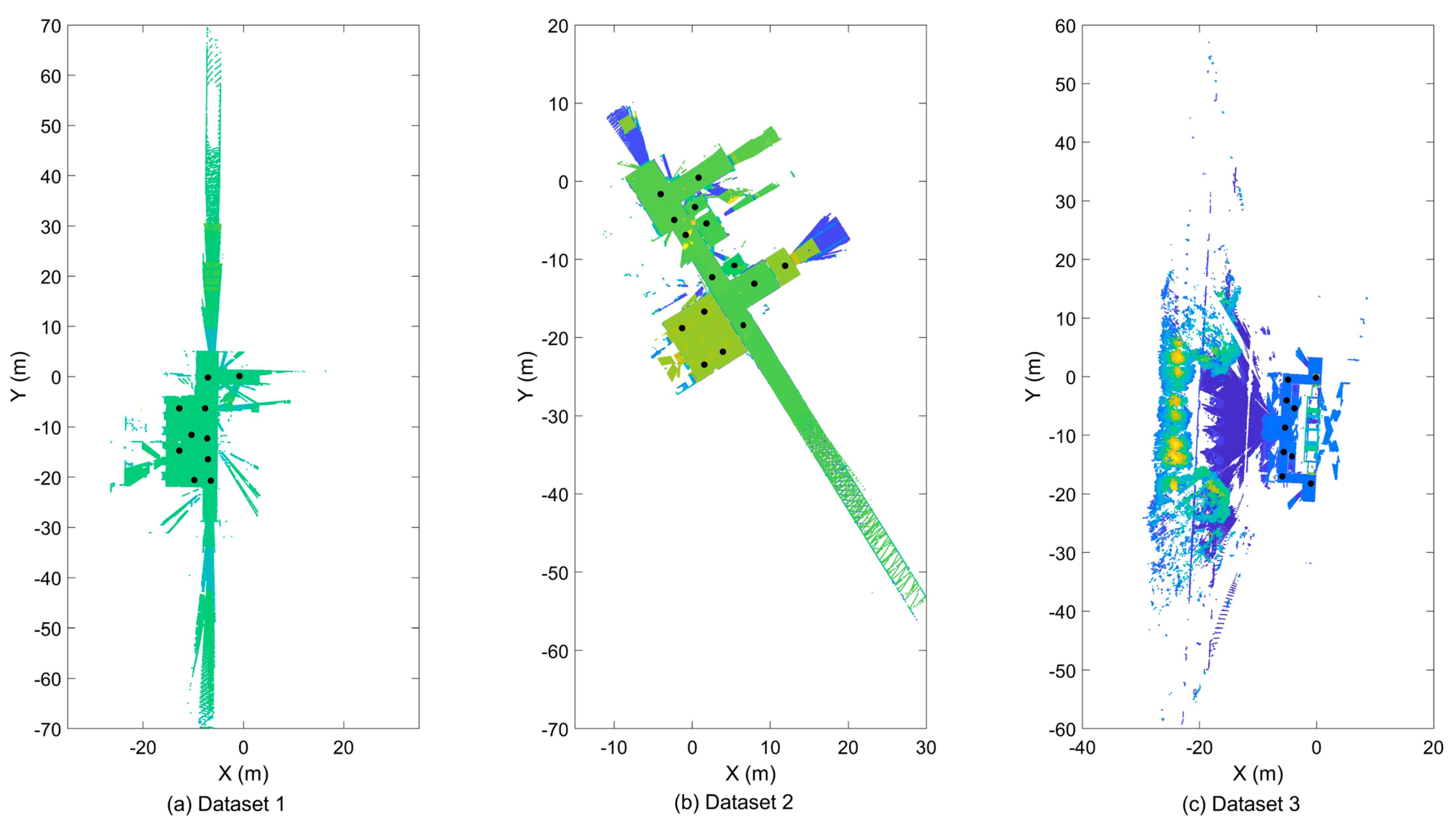
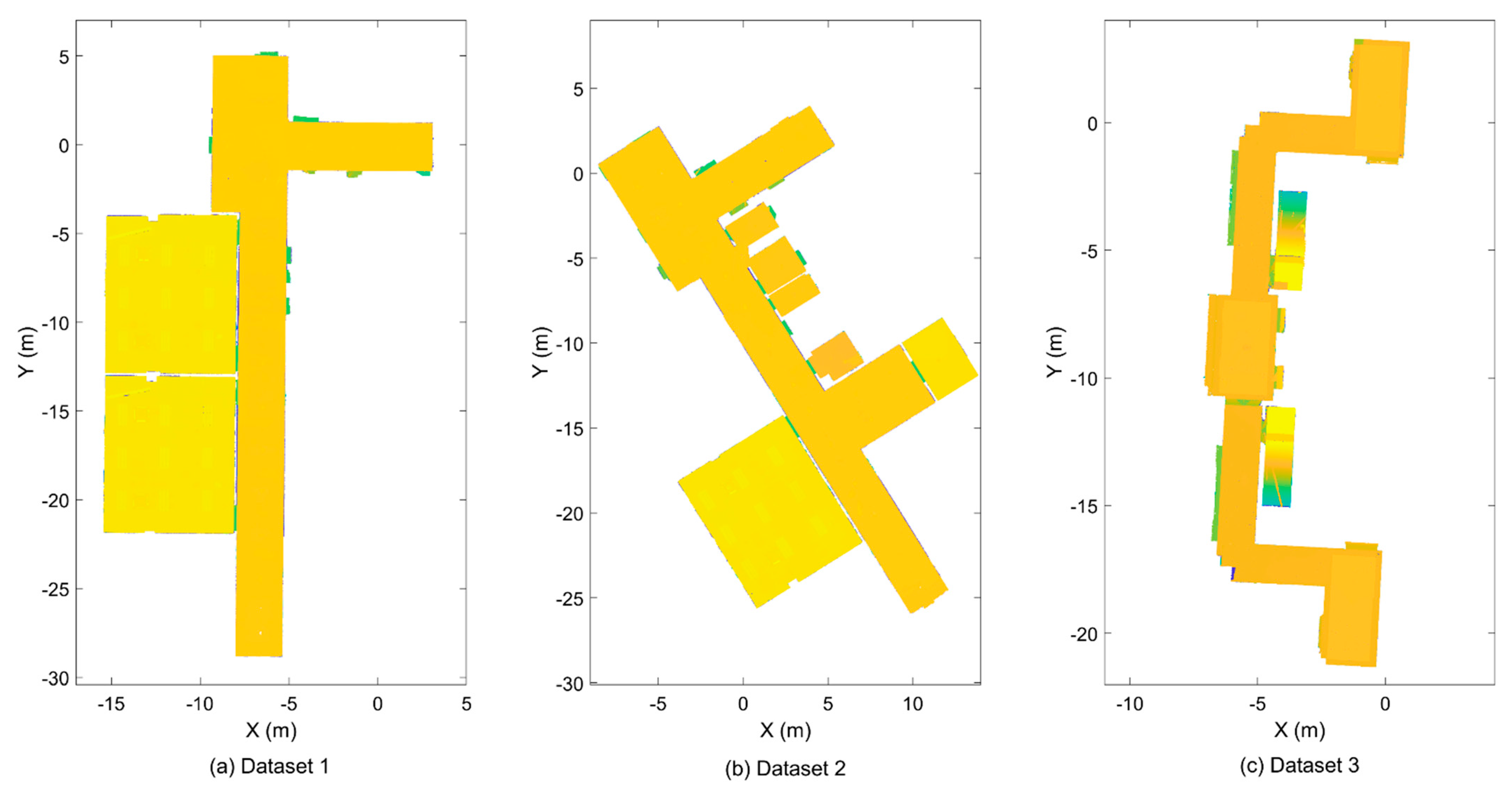
2.1. Study Sites and Data
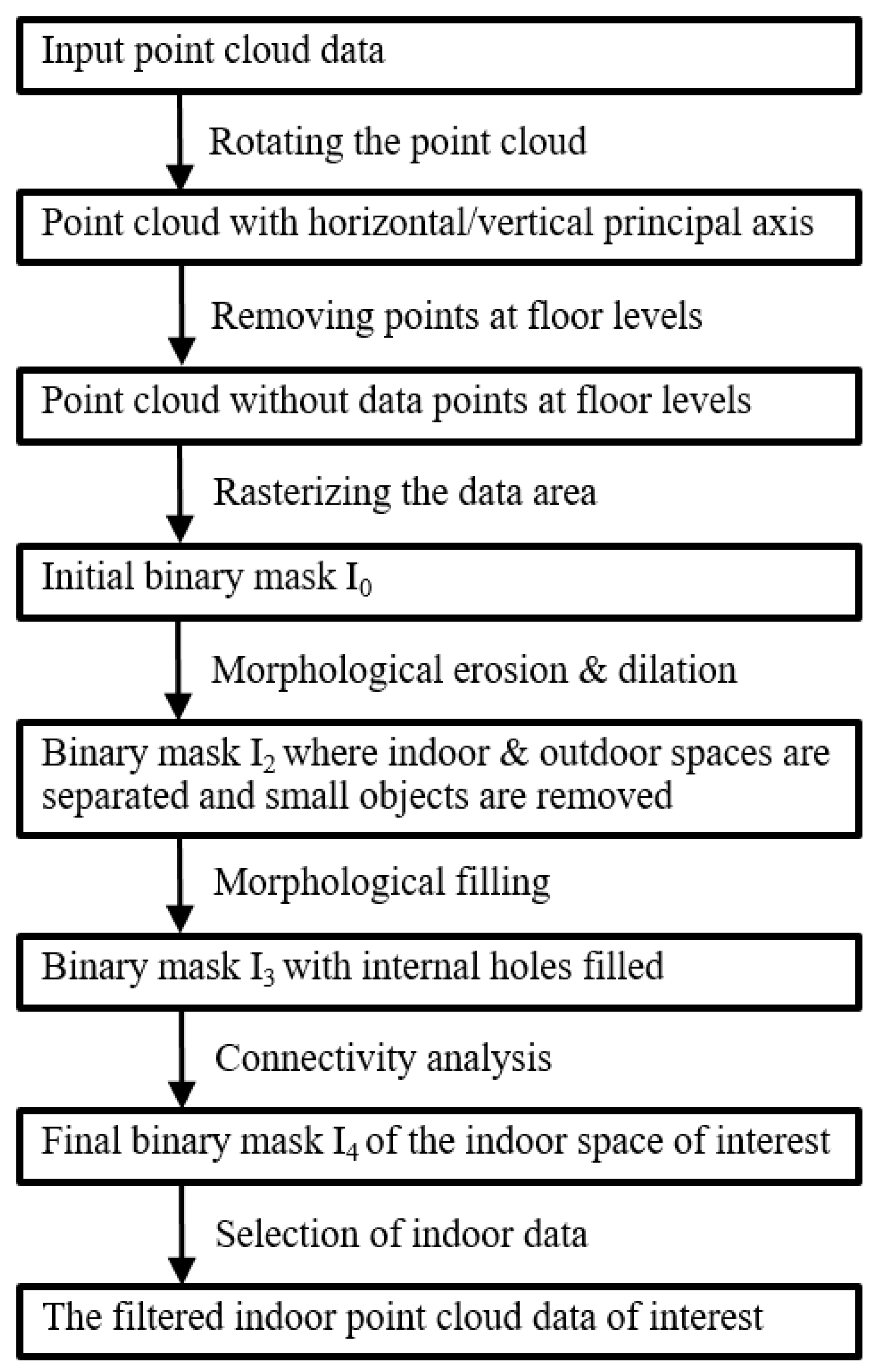
Multiple sets of point cloud data representing the indoor space of buildings were tested for the approach proposed. However, due to the similarity of the spatial confirmations of the buildings, three representative datasets are reported in this article. In dataset 1, the targeted objects during the surveying include one corridor and two large rooms. In dataset 2, there are several small rooms in addition to one corridor and one large room. Dataset 3 represents the corridor at the building entrance and two small storage rooms. These datasets were acquired using a Leica RTC360 scanner at multiple scanner stations. The point cloud data obtained from each station were registered using the Leica Cyclone software. The registered point clouds have extremely high spatial densities (over 300 million data points). For ease of visualization, these datasets were downsampled using a minimum distance of 20 mm between data points.
Figure 1 shows the thinned point cloud data, which consist of approximately 1.9 million, 2.0 million, and 1.4 million data points, respectively. The color information represents the elevations of the data points. By observation, various subsets of the data points were located outside the indoor region of interest in each dataset, especially in dataset 3, where lots of outdoor objects were recorded due to the presence of several large façade windows at the building entrance.

2.2. Methodology

The basic idea of the approach investigated in this study is the following. The bounding planar area covering all data points projected to a plane is partitioned into square sub-areas of equal side length r. Data points are indexed to individual sub-areas. A companying binary mask image of the same spatial range and resolution as the whole partitioned area is created to show the status (either occupied or empty) of individual sub-areas. The binary mask image is updated through a sequence of mathematical morphological operations, followed by a connectivity analysis to identify the largest object(s). These lead to the final mask corresponding to the indoor space of interest, which is used as a filter to select the indoor data points of interest. These steps of the approach are illustrated in Figure 2 and elaborated in Section 2.2.1, Section 2.2.2, Section 2.2.3, Section 2.2.4, Section 2.2.5, Section 2.2.6 and Section 2.2.7.

2.2.1. Data Pre-Processing

As the data filtering using the binary mask is pixel-based, data points at boundaries may be in the saw-blade shape. To avoid or minimize this defect, the original point cloud data can be rotated about the plumb direction so that the predominant orientations of the data are parallel to either x or y axis. The rotated point cloud is used only for deriving the final binary mask that consists of exactly two classes (i.e., indoor and outdoor data points). Once the class of each data point is known, the classification information is applied directly to the original point cloud.
The rotation can readily be applied using commercial or open-source software, such as Leica Cyclone and CloudCompare. Alternatively, the following RANSAC-based (i.e., random sample consensus) algorithm can be considered, which was used in this study. A random subsample (e.g., 10% of the total data points) is used for computational efficiency. In the algorithm, the normal of each individual data point selected was calculated, which is followed by the selection of those (referred to as V) almost perpendicular to the vertical axis. An individual normal vector v out of the set V was randomly selected, followed by the calculation of a unit vector (referred to as u) perpendicular to v on the xy plane. For each individual normal remaining in V, its angles to v and u are calculated, the minimum value (referred to as α) of which was taken. Repeating this for every normal (except v) in V leads to a vector (referred to as A) of α values. The number of values (in A) that are smaller than a pre-defined threshold (e.g., 0.001 rad in this study) is counted and represented by m. The aforementioned steps (i.e., the random selection of v and the subsequent steps) are repeated in a large number of times (e.g., 100,000 times in this study). The α corresponding to the maximum value of m is used for rotating the point cloud.

2.2.2. Removal of Data Points at the Floor Level

It was found essential to remove the data points near the floor level before the partition is implemented in Section 2.2.3. This is to account for the cases where chunks of data points exist continuously from the indoor area of interest to either an outdoor area (e.g., entrances at the ground floor) or to another unwanted indoor area. To achieve this, the following data processing is considered. The data points below the average elevation of all data points are selected. The M-estimator sample consensus algorithm [46] with an orientation constraint (i.e., a vertical normal) is used to find the floor plane. The maximum distance from inlier points to the floor plane fitted can be set to a reasonably large value (e.g., 0.2 m used in this study) to ensure that all the data points close to the floor level are selected and subsequently removed.

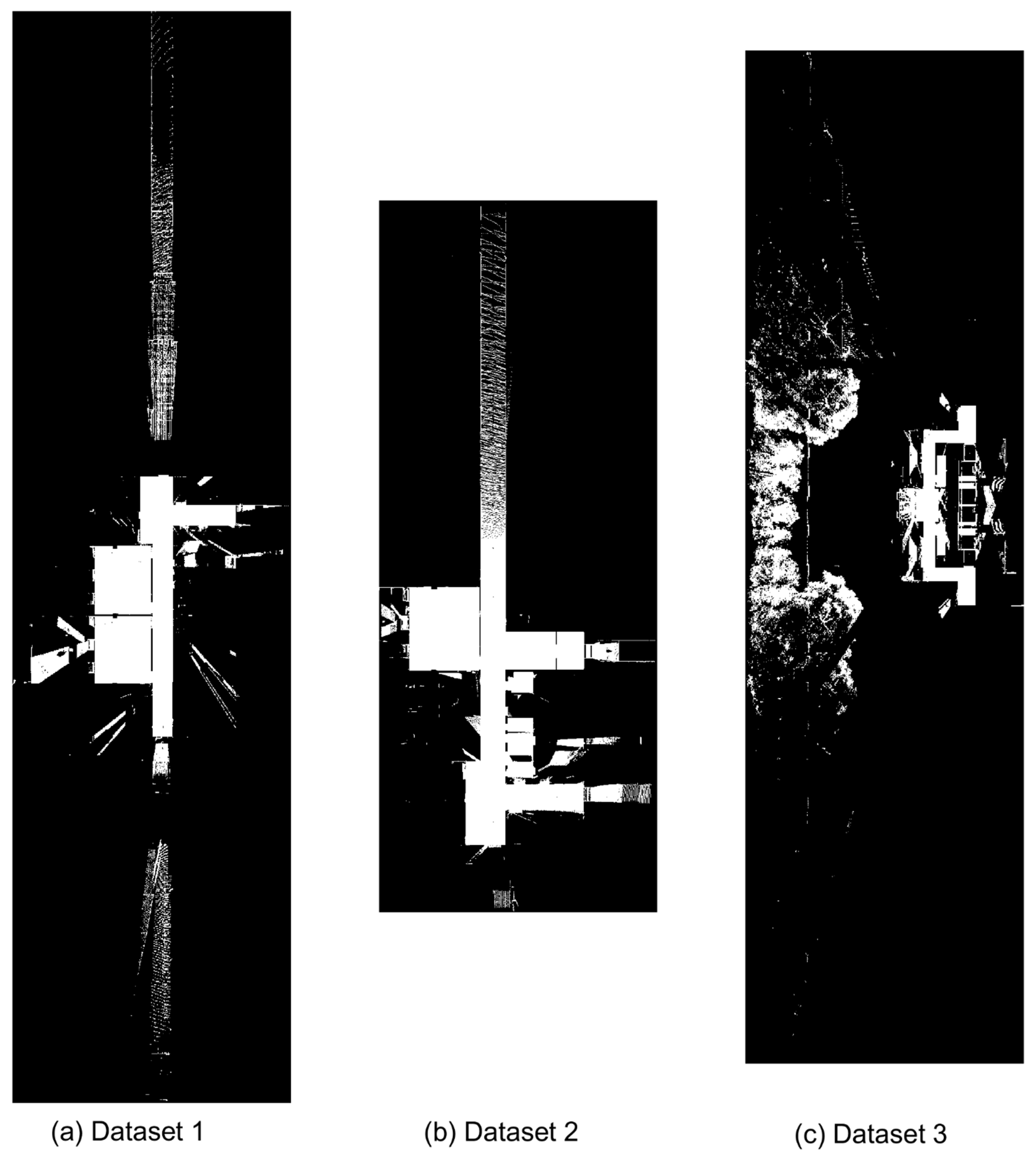
2.2.3. Pixilation of the Data Area

The data area represents the spatial extent of the whole point cloud data projected onto the xy plane. It is a rectangular shape, the length and width of which are determined by the ranges of the whole data in x and y directions. An initial binary mask image I0 is created by rasterizing the rectangular area. This raster image consists of pixels that have one of exactly two cases: occupied pixel (i.e., occupied by at least one data point) and empty pixel. The values of the pixels are set to 1 for the occupied and 0 for the empty.
The introduction of the approach is based on the data projection to the xy plane, which is obviously the most important case. However, the same procedure can also be applied to the data that are projected onto any other planes. For example, data projection onto xz or yz plane can be considered for removing data points above the ceiling and/or below the floor.

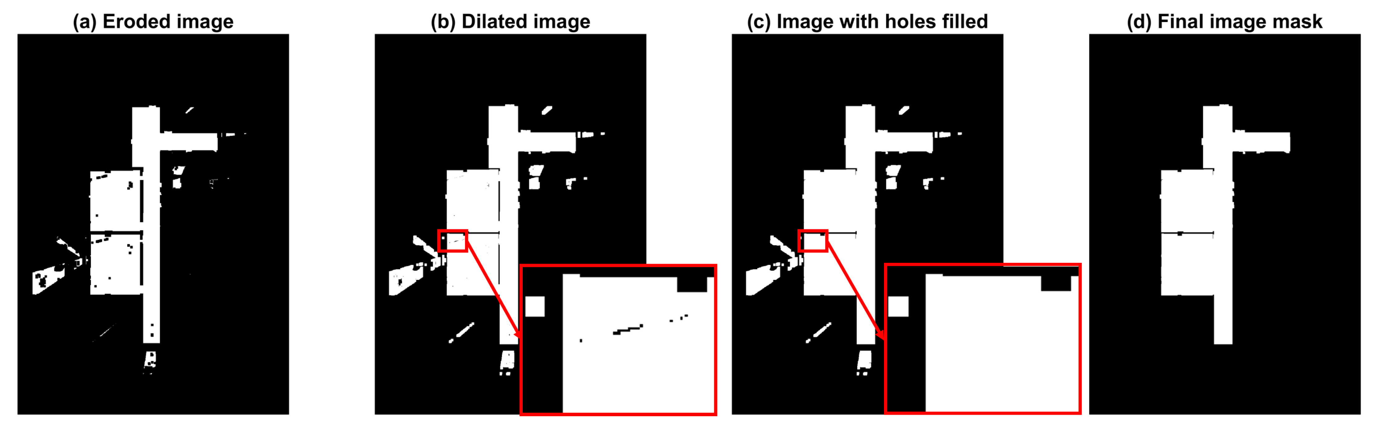
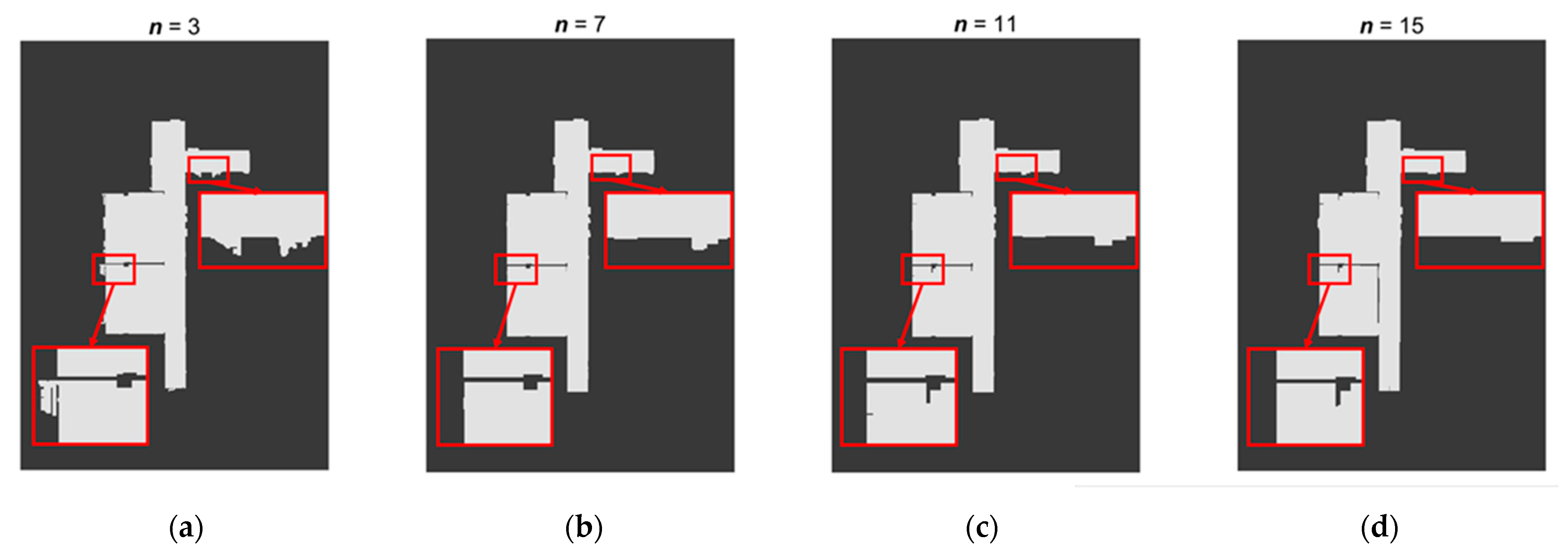
2.2.4. Morphological Erosion and Dilation

The mathematical morphological operations considered in this study mainly include binary erosion and binary dilation (i.e., MATLAB Image Processing Toolbox functions: imerode and imdilate, respectively [47]). The former removes pixels to the boundaries of objects in an input image, while dilation adds pixels on object boundaries. These operations lead to an output image of the same size (as the input one), where the value of each pixel in the output image is based on the corresponding pixel and its neighbors in the input image. Detailed information (including the theoretical background) on morphological erosion and dilation can be found in References [35,36,48].
To enable these operations, a structuring element (SE) in the form of a matrix is required to probe the input image. Its center identifies the pixel (in the input image) being processed. Meanwhile, its size and shape determine the neighborhood used in the processing of each pixel identified, and the number of pixels removed from or added to object boundaries in an image. For a binary image, such as the ones used in this study, a flat SE is required. It is a binary valued (i.e., true or false) neighborhood, where the true pixels are included in the morphological computation, and the false pixels are not. The SE can be in different shapes, including but not limited to diamond, disk, rectangle, square, or line shape, for 2D morphological operations, and cubic, cuboidal, or spherical shapes for 3D cases. In this study, a square flat SE of the size n was used, which is suitable for the datasets considered. In addition, it is assumed that all the neighboring pixels of the images were considered, and, as such, all the pixels in the SE were set to be true.
For erosion of a binary image, a pixel of the output image is set to 0 if any of the neighboring pixels specified by a SE in the input image have the value 0. For the dilation, a pixel is set to 1 if any of the neighboring pixels specified by a SE have the value 1.
The processing started with a morphological erosion applied to the input image I0, which results in an eroded image I1. This is followed by a morphological dilation, leading to a dilated image I2. These two steps can remove small objects in the input image and break the connections at the indoor-outdoor interfaces. It should be noted that the data points with comparatively large spacing (compared to the pixel size of the binary mask image) can also be removed because they are treated as small individual objects in the morphological erosion. A suitable value of n is affected by the complexities of the occupied pixels at boundaries, and often varies from one case to another. As such, trial tests on different values of n are needed for determining a suitable/optimal one, which can be confirmed by an observation of the filtered point cloud data.

2.2.5. Hole Filling

There may be empty pixels (such as small internal holes) surrounded by occupied pixels in the binary mask, either because the point cloud used for deriving the initial binary mask does not have any data points at those pixel locations or as a result of the morphological erosion in which sparse data points are removed. Such internal holes (if any) should be filled to ensure that all the indoor area is fully covered, which lead to an updated mask image I3. In this research, this is achieved using morphological reconstruction (i.e., MATLAB Image Processing Toolbox function: imfill [47]), the detailed information of which can be found in References [33,36]. In the reconstruction, a hole is a set of background pixels that cannot be reached by filling in the background from the edge of the image. The holes in the image (i.e., I2) are filled through the reconstruction by choosing a marker image F to be 0 everywhere, expect on the image border, where it is set to 1-I2 [36].

2.2.6. Connectivity Analysis

The purpose of the connectivity analysis is to group the occupied pixels into different objects. In this research, two adjoining pixels are assumed to be part of the same object if they are both on and are connected along the horizontal or vertical direction. A 3-by-3 connectivity matrix M can be considered, consisting of the value 1 for all the elements in its second row and the second column, and 0 for the four corner elements of M (i.e., 4-connected or 4 neighborhood connectivity). The 1-valued elements in M define neighborhood locations relative to the center element of the connectivity.
An indoor area is typically surveyed from a set of successive scanner stations. As such, the point cloud data representing indoor rooms scanned are often continuous. In this case, the largest object in the binary image I3 can be extracted in the connectivity analysis (i.e., MATLAB Image Processing Toolbox function: bwareafilt [47]), which lead to the final mask image I4. However, in rare cases where indoor data are not continuous, multiple largest objects representing the indoor space of interest might need to be extracted, which can be determined by observation. The largest object(s) extracted constitute the final mask image.

2.2.7. Selection of Indoor Data

The final mask image I4 is overlaid on the rotated point cloud data. A true-or-false index is created for all data points by checking their locations in I4. Those located in the spatial ranges of 1-valued pixels of I4 are flagged as true, and otherwise false. This index is subsequently applied to the original point cloud to select the indoor data points of interest.

3. Results

As mentioned in Section 1, several potential filtering approaches, such as cluster-based segmentation and classification, statistical outlier removal (SOR), and the plane fitting-based classification, had been tested for the problem considered. However, it was found that none of these approaches could successfully separate the outdoor data from the indoor data of interest and produce comparable results as those obtained using the approach investigated in this research. This is probably because such existing methods were not developed to solve the particular problem considered in this research.
Apart from that, the rotation of the point cloud data in the pre-process was realized in C++; all the other data processing steps were executed in MATLAB, where relevant image processing tools are available for carrying out the morphological operations required. The initial binary mask images I0 for the three datasets (using the rotated point cloud data) are shown in Figure 3. The sizes of the images depend on the spatial ranges of the data and vary for the datasets considered. There are empty pixels at the locations where data points are present in the initial point cloud data shown in Figure 1. This is because the data points near the floor level were removed (as stated in Section 2.2.2) before the mask image was created.
Dataset 1 was used as an example to illustrate the outputs of the steps presented in Section 2.2.4, Section 2.2.5, Section 2.2.6 and Section 2.2.7, which are shown in Figure 4. It should be noted that the images in Figure 4 are trimmed versions (i.e., some black-colored margin were not shown) of the original for better visualization. As shown in Figure 4a, most of the outdoor data regions shown in Figure 3a were removed after the morphological erosion. In addition, some spatially continuous data regions at the indoor-outdoor interfaces were separated. Figure 4b depicts the image after the morphological dilation was applied to recover the footprint of the indoor space of interest. As expected and observed in Figure 4b, some small holes in the eroded image I1 were completely filled during the morphological dilation, while relatively large holes were only partially filled. The remaining holes in the dilated image I2 were filled using the morphological reconstruction algorithm [33,36], which lead to I3 shown in Figure 4c. It can be seen that there are several objects in I3, including the largest one that needs to be extracted and several small ones. Figure 4d shows the largest object extracted in the connectivity analysis, which was the final image I4 used for selecting the indoor data of interest.
The effect of the SE size (i.e., the number of elements/pixels) on the I4 was investigated. For dataset 1, the I4 obtained for n = 3, 5, 7, and 9 is shown in Figure 5a–d, respectively. It was found that more data points at the boundary could potentially be filtered out using a larger SE size. Theoretically, when the value of n is too small, some outdoor data points adjoining to the boundary might not adequately be removed. On the other side, when the value of n is too large, some local indoor data points at the boundary could also be lost. These inferences were confirmed by the results shown in Figure 5. However, the effects were found to be relatively small and may be considered acceptable depending on the actual applications of the filtered indoor data. If more accurate results are required, a trade-off between the removal of outdoor data and the preservation of indoor data needs to be considered. To find the optimal value of n, it is recommended that a range of n values be tested for any particular dataset considered. This is a reasonable approach to find a preferred value of n as the approach proposed in this study is efficient (referring to the last paragraph of Section 3). For dataset 1, n = 7 was found to be adequate to remove the outdoor data, while the full footprint of the indoor data of interest was successfully kept. As introduced in Section 2.2.4, the same SE shape (a square flat SE) was suitable for the datasets considered. As such, the other SE shapes were not analyzed here. However, SE of different shapes might be useful for non-Manhattan world structures, the selection of which will depend on the geometric characteristics of buildings.
In addition to the SE size, the pixel width of the binary mask image can affect which data points to be removed. To show its effects on the binary image generated, an example is illustrated in Figure 6, where only a small indoor space (i.e., the top room in Figure 3a) of dataset 1 was shown for a better visualization. When the pixel width is too small (e.g., Figure 6a,b), it is likely to result in many scattered empty pixels within the indoor space of interest during the pixilation of the data area descried in Section 2.2.3. These empty pixels could lead to the majority of occupied pixels being removed in the morphological erosion. Therefore, the pixel width set for the I0 should be larger than the local data spacing. For the thinned point cloud data of approximately uniform spatial distribution in this study, it was found that 50 mm (i.e., 2.5 times the average data spacing of 20 mm, as demonstrated in Figure 6) was large enough to capture all the local indoor areas of interest. This value should also be suitable for the original point clouds (i.e., before downsampling) as their local data spacings are not larger than those of the thinned ones. On the other side, when the pixel size was too large (i.e., a coarse resolution), an increasing level of local outdoor data areas at the exterior boundaries of the buildings might not be distinguished from the indoor area, and, as such, more outdoor data may be included in the post-filtering point clouds. As such, it is also recommended that parametric study be carried out for a particular dataset for deriving a suitable pixel size.
In addition to the overwhelming majority of outdoor data shown on the xy plane (Figure 1), it was also observed that a small amount of scattered noisy data points existing above the ceiling and/or below the floor. Most of these noisy data were caused by the small space for accommodating lighting equipment at the site considered. To remove or reduce those, the same filtering approach can be applied to the data points (Figure 7a) that are obtained using the xy binary mask image and projected to an elevation plane (e.g., the yz plane). The SE size used for the erosion and dilation was also n = 7. Figure 7b shows the final point cloud data after the binary mask images for both xy and yz projections were applied to dataset 1. It was observed that the outdoor data were successfully removed. The openings on the walls are clearly shown, including windows (i.e., those on the left side of the data in Figure 7) and doors (if opened). The data points within the indoor space (e.g., furniture in the rooms) were also preserved.
For dataset 2 and dataset 3, the SE sizes used for the data projected to the xy plane were 11 and 17, respectively. The SE sizes used for the yz projection are 5 for dataset 2 and 7 for dataset 3. Meanwhile, the same pixel size of 50 mm was used for creating I0. A summary of the values of the key variables used is shown in Table 1. The data processing suggests that the size of SE varied for different datasets to achieve preferred output point clouds. The main reason to adjust the SE values is to obtain the optimal results, although we also found that consistent results were obtained when the same SE values was used (e.g., the SE size of 7) for all the datasets. The adjustment is reasonable given the fact that the approach used can be implemented very efficiently. For an individual dataset, the same SE size was used for both erosion and dilation. It should be noted that it is also possible to use a larger SE size for dilation than that used for erosion if more data (e.g., those represent the window or door frames) at the building boundary need to be included.
The filtered point clouds for the datasets considered are shown in Figure 8, in which planar views are adopted for better visualization. These results confirm that the indoor data of interest were accurately kept. To assess the quality of the filtering, the output point clouds were compared to the ground truth indoor data that were manually labeled using three indices: precision (=TP/(TP + FP)), recall (=TP/(TP + FN)), and F1-score (=2/(1/recall + 1/precision) = 2 × TP/(2 × TP + FP +FN)), where TP, FP, FN represent true positives, false positives, false negatives, respectively. The values of these indices for all the datasets considered are shown in Table 1. The average precision is 99.50%, confirming the high quality of the filtering.
Using an average office computer (4 cores of i5-7440HQ CPU, 16GB RAM), the total times taken in MATLAB for processing datasets 1, 2, and 3 are 0.53, 0.48, and 0.33 s, respectively, suggesting that the approach proposed is computationally efficient. It should be noted that these values do not include the time taken for the point cloud rotation in the data pre-processing (approximately 0.79, 0.77, and 0.48 s for datasets 1, 2, and 3, respectively, using the RANSAC-based algorithm described in Section 2.2.1).
There may be a challenge in applying the method proposed to clean the outdoor data points immediately above ceilings when there are multiple ceilings at different levels. This is because the outdoor data points above a lower-level ceiling may be occluded by the indoor data points below a higher-level ceiling in the data projection. In this case, the occluded outdoor data cannot be distinguished from the indoor data by our method. To avoid or minimize the occlusion situations, it is necessary to choose an appropriate direction of point cloud data projection. This is certainly achievable for leveled ceilings but might be challenging for inclined ceilings. It should be noted that these challenges typically occur in the cases where there are openings in ceilings so that some point cloud data above ceilings may be recorded. However, such issues do not normally exist in most cases where ceilings are solid surfaces.
This study demonstrated the application of the method proposed to Manhattan-world buildings. This limitation is due to the fact that a fixed SE shape (i.e., rectangular) was considered. However, the method has the potential to be extended to non-Manhattan world structures. To this end, SE of a different shape needs to be explored, taking into account the geometric characteristics of the boundaries of each building, which is likely to be a case-by-case investigation. For example, a disk-shaped SE may suit the buildings with curved walls, while a diamond-shaped SE may be suitable for those with polygonal walls. It is also possible to specify a SE of any other shapes. As such, it will be interesting to explore the automatic generation of a suitable SE (shape and size) according to the building geometric characteristics in a future study.

4. Conclusions

An efficient approach was introduced for filtering out outdoor point cloud data in the applications where the indoor data of Manhattan-world buildings are of interest. In this approach, a binary mask image was created and updated through a series of morphological operations and image processing, mainly including pixilation of the data area, binary erosion, binary dilation, hole filling, and connectivity analysis. The final version of the binary mask was used as a filter to select the data points in the indoor space of interest.
The approach was tested against the three point-cloud datasets representing buildings of varying spatial confirmations. The effects of the image pixel size and the SE size on the final outputs were discussed. For the datasets considered, it was found the pixel size that is 2.5 times the average data spacing was adequate to capture all the local indoor areas of interest. The execution of the approach in an average office computer confirms its computational efficiency (0.53, 0.48, and 0.33 s for datasets 1, 2, and 3, respectively). Based on visual inspections and the set of quality indices (precision = 99.50%, recall = 98.73%, and F1-score = 99.11% on average) calculated, the method demonstrates its ability to effectively keep the indoor data points of interest.
A future study can be focused on the application of the approach to non-Manhattan world structures. In this case, structure elements of different shapes need to be explored, depending on the geometric characteristics of building boundaries.

Author Contributions

Conceptualization, L.F.; methodology, L.F. and Y.C.; validation, L.F. and Y.C.; formal analysis, L.F. and Y.C.; data curation, Y.C.; writing—original draft preparation, L.F.; writing—review and editing, L.F.; visualization, L.F. and Y.C.; project administration, L.F.; funding acquisition, L.F. All authors have read and agreed to the published version of the manuscript.

Funding

This research was funded by Xi’an Jiaotong-Liverpool University Key Program Special Fund, grant number KSF-E-40, and Xi’an Jiaotong-Liverpool University Research Development Fund, grant number RDF-18-01-40.

Data Availability Statement

The data presented in this study are available on request from the corresponding author.

Conflicts of Interest

The authors declare no conflict of interest.

References

  1. Liu, M.Y.; Chen, R.Z.; Li, D.R.; Chen, Y.J.; Guo, G.Y.; Cao, Z.P.; Pan, Y.J. Scene Recognition for Indoor Localization Using a Multi-Sensor Fusion Approach. Sensors 2017, 17, 2847. [Google Scholar] [CrossRef] [Green Version]
  2. Guo, S.; Xiong, H.J.; Zheng, X.W. A Novel Semantic Matching Method for Indoor Trajectory Tracking. ISPRS Int. J. Geo-Inf. 2017, 6, 197. [Google Scholar] [CrossRef]
  3. Hamieh, A.; Makhlouf, A.B.; Louhichi, B.; Deneux, D. A BIM-based method to plan indoor paths. Autom. Constr. 2020, 113, 103120. [Google Scholar] [CrossRef]
  4. Tarihmen, B.; Diyarbakirli, B.; Kanbur, M.O.; Demirel, H. Indoor navigation system of faculty of civil engineering, ITU: A BIM approach. Balt. J. Mod. Comput. 2020, 8, 359–369. [Google Scholar] [CrossRef]
  5. Tekavec, J.; Lisec, A. 3D Geometry-Based Indoor Network Extraction for Navigation Applications Using SFCGAL. ISPRS Int. J. Geo-Inf. 2020, 9, 417. [Google Scholar] [CrossRef]
  6. Nikoohemat, S.; Diakité, A.A.; Zlatanova, S.; Vosselman, G. Indoor 3D reconstruction from point clouds for optimal routing in complex buildings to support disaster management. Autom. Constr. 2020, 113, 103109. [Google Scholar] [CrossRef]
  7. Ma, G.; Wu, Z. BIM-based building fire emergency management: Combining building users’ behavior decisions. Autom. Constr. 2020, 109, 102975. [Google Scholar] [CrossRef]
  8. Wang, R.; Xie, L.; Chen, D. Modeling indoor spaces using decomposition and reconstruction of structural elements. Photogramm. Eng. Remote Sens. 2017, 83, 827–841. [Google Scholar] [CrossRef]
  9. Heaton, J.; Parlikad, A.K.; Schooling, J. Design and development of BIM models to support operations and maintenance. Comput. Ind. 2019, 111, 172–186. [Google Scholar] [CrossRef]
  10. Fan, L.; Powrie, W.; Smethurst, J.; Atkinson, P.; Einstein, H. The effect of short ground vegetation on terrestrial laser scans at a local scale. ISPRS J. Photogramm. Remote Sens. 2014, 95, 42–52. [Google Scholar] [CrossRef] [Green Version]
  11. Fan, L. A comparison between structure-from-motion and terrestrial laser scanning for deriving surface roughness: A case study on a sandy terrain surface, The International Archives of the Photogrammetry. Remote Sens. Spat. Inf. Sci. 2020, 42, 1225–1229. [Google Scholar]
  12. Lau, L.; Quan, Y.; Wan, J.; Zhou, N.; Wen, C.; Qian, N.; Jing, F. An autonomous ultra-wide band-based attitude and position determination technique for indoor mobile laser scanning. ISPRS Int. J. Geo-Inf. 2018, 7, 155. [Google Scholar] [CrossRef] [Green Version]
  13. Lichti, D.D.; Jarron, D.; Tredoux, W.; Shahbazi, M.; Radovanovic, R. Geometric modelling and calibration of a spherical camera imaging system. Photogramm. Rec. 2020, 35, 123–142. [Google Scholar] [CrossRef]
  14. Sanhudo, L.; Ramos, N.M.; Martins, J.P.; Almeida, R.M.; Barreira, E.; Simões, M.L.; Cardoso, V. A framework for in-situ geometric data acquisition using laser scanning for BIM modelling. J. Build. Eng. 2020, 28, 101073. [Google Scholar] [CrossRef]
  15. Sun, Y.; Schaefer, S.; Wang, W. Denoising point sets via L0 minimization. Comput. Aided Geom. Des. 2015, 35, 2–15. [Google Scholar] [CrossRef]
  16. Mattei, E.; Castrodad, A. Point Cloud Denoising via Moving RPCA. Comput. Graph. Forum 2016, 36, 123–137. [Google Scholar] [CrossRef]
  17. Han, X.F.; Jin, J.S.; Wang, M.J.; Jiang, W.; Gao, L.; Xiao, L. A review of algorithms for filtering the 3D point cloud. Signal Process. Image Commun. 2017, 57, 103–112. [Google Scholar] [CrossRef]
  18. Chen, H.; Wei, M.; Sun, Y.; Xie, X.; Wang, J. Multi-Patch Collaborative Point Cloud Denoising via Low-Rank Recovery with Graph Constraint. IEEE Trans. Vis. Comput. Graph. 2020, 26, 3255–3270. [Google Scholar] [CrossRef]
  19. Kurdi, F.T.; Awrangjeb, M.; Munir, N. Automatic filtering and 2D modeling of airborne laser scanning building point cloud. Trans. GIS 2020, 25, 164–188. [Google Scholar] [CrossRef]
  20. Huber, D.; Akinci, B.; Adan, A.; Anil, E.B.; Okorn, B.; Xiong, X. Methods for automatically modeling and representing as-built building information models. In Proceedings of the NSF Engineering Research and Innovation Conference, Atlanta, GA, USA, 4 January 2021. [Google Scholar]
  21. Oesau, S.; Lafarge, F.; Alliez, P. Indoor scene reconstruction using feature sensitive primitive extraction and graph-cut. ISPRS J. Photogramm. Remote Sens. 2014, 90, 68–82. [Google Scholar] [CrossRef] [Green Version]
  22. Okorn, B.; Xiong, X.; Akinci, B.; Huber, D. Toward Automated Modeling of Floor Plans. In Proceedings of the Symposium on 3D Data Processing, Visualization and Transmission, Paris, France, 18–20 May 2010. [Google Scholar]
  23. Mura, C.; Mattausch, O.; Pajarola, R. Piecewise-planar reconstruction of multi-room interiors with arbitrary wall arrangements. Comput. Graph. Forum 2016, 35, 179–188. [Google Scholar] [CrossRef]
  24. Ochmann, S.; Vock, R.; Wessel, R.; Klein, R. Automatic reconstruction of parametric building models from indoor point clouds. Comput. Graph. 2016, 54, 94–103. [Google Scholar] [CrossRef] [Green Version]
  25. Ochmann, S.; Vock, R.; Klein, R. Automatic reconstruction of fully volumetric 3D building models from oriented point clouds. ISPRS J. Photogramm. Remote Sens. 2019, 151, 251–262. [Google Scholar] [CrossRef] [Green Version]
  26. Macher, H.; Landes, T.; Grussenmeyer, P. From point clouds to building information models: 3D semi-automatic reconstruction of indoors of existing buildings. Appl. Sci. 2017, 7, 1030. (In Switzerland) [Google Scholar] [CrossRef] [Green Version]
  27. Frías, E.; Balado, J.; Díaz-Vilariño, L.; Lorenzo, H. Point cloud room segmentation based on indoor spaces and 3D mathematical morphology. Int. Arch. Photogramm. Remote Sens. Spat. Inf. Sci. 2020, XLIV-4/W1-2020, 49–55. [Google Scholar]
  28. Pintore, G.; Mura, C.; Ganovelli, F.; Fuentes-Perez, L.; Pajarola, R.; Gobbetti, E. State-of-the-art in Automatic 3D Reconstruction of Structured Indoor Environments. Comput. Graph. Forum 2020, 39, 667–699. [Google Scholar] [CrossRef]
  29. Cai, Y.; Fan, L. An efficient approach to automatic construction of 3d watertight geometry of buildings using point clouds. Remote Sens. 2021, 13, 1947. [Google Scholar] [CrossRef]
  30. Kim, S.; Manduchi, R.; Qin, S. Multi-planar monocular reconstruction of manhattan indoor scenes. In Proceedings of the 2018 International Conference on the 3D Vision, 3DV 2018, Verona, Italy, 5–8 September 2018; pp. 616–624. [Google Scholar] [CrossRef] [Green Version]
  31. Matheron, G.; Serra, J. The birth of mathematical morphology. In Proceedings of the 6th Intl. Symp. Mathematical Morphology, Sydney, Australia, 3–5 April 2002; pp. 1–16. [Google Scholar]
  32. Serra, J. Image Analysis and Mathematical Morphology; Academic Press: London, UK, 1982. [Google Scholar]
  33. Soille, P. Morphological Image Analysis: Principles and Applications; Springer: Berlin/Heidelberg, Germany, 1999. [Google Scholar]
  34. Blaschke, T. Object based image analysis for remote sensing. ISPRS J. Photogramm. Remote Sens. 2010, 65, 2–16. [Google Scholar] [CrossRef] [Green Version]
  35. Rishikeshan, C.A.; Ramesh, H. An automated mathematical morphology driven algorithm for water body extraction from remotely sensed images. ISPRS J. Photogramm. Remote Sens. 2018, 146, 11–21. [Google Scholar] [CrossRef]
  36. Gonzalez, R.C.; Woods, R.E.; Eddins, S.L. Digital Image Processing Using MATLAB, 3rd ed.; Gatesmark Publishing: Knoxville, TN, USA, 2020. [Google Scholar]
  37. Serra, J.; Soille, P. Mathematical Morphology and Its Applications to Image Processing; Springer Science +Business Media: Berlin, Germany, 2012. [Google Scholar]
  38. Balado, J.; Oosterom, P.V.; Díaz-Vilariño, L.; Meijers, M. Mathematical morphology directly applied to point cloud data. ISPRS J. Photogramm. Remote Sens. 2020, 168, 208–220. [Google Scholar] [CrossRef]
  39. Serna, A.; Marcotegui, B. Detection, segmentation and classification of 3D urban objects using mathematical morphology and supervised learning. ISPRS J. Photogramm. Remote Sens. 2014, 93, 243–255. [Google Scholar] [CrossRef] [Green Version]
  40. Rodríguez-Cuenca, B.; García-Cort´es, S.; Ord´onez, C.; Alonso, C.M. Morphological operations to extract urban curbs in 3D MLS point clouds. ISPRS Int. J. Geo-Inf. 2016, 5, 93. [Google Scholar] [CrossRef]
  41. Balado, J.; Díaz-Vilariño, L.; Arias, P.; González-Jorge, H. Automatic classification of urban ground elements from mobile laser scanning data. Autom. Constr. 2018, 86, 226–239. [Google Scholar] [CrossRef] [Green Version]
  42. Balado, J.; Díaz-Vilarino, L.; Arias, P.; Lorenzo, H. Point clouds for direct pedestrian pathfinding in urban environments. ISPRS J. Photogramm. Remote Sens. 2019, 148, 184–196. [Google Scholar] [CrossRef]
  43. Li, Y.; Yong, B.; Van Oosterom, P.; Lemmens, M.; Wu, H.; Ren, L.; Zheng, M.; Zhou, J. Airborne LiDAR data filtering based on geodesic transformations of mathematical morphology. Remote Sens. 2017, 9, 1104. [Google Scholar] [CrossRef] [Green Version]
  44. Gorte, B.; Pfeifer, N. Structuring laser-scanned trees using 3D mathematical morphology. ISPRS Int. Arch. Photogramm. Remote Sens. 2004, 35, 929–933. [Google Scholar]
  45. Bucksch, A.; Wageningen, H. Skeletonization and segmentation of point clouds using octrees and graph theory. In Proceedings of the ISPRS Symposium: Image Engineering and Vision Metrology, Dresden, Germany, 25–27 September 2006; Volume XXXVI. [Google Scholar] [CrossRef]
  46. Torr, P.H.S.; Zisserman, A. MLESAC: A New Robust Estimator with Application to Estimating Image Geometry. Comput. Vis. Image Underst. 2000, 78, 138–156. [Google Scholar] [CrossRef] [Green Version]
  47. MATLAB Image Processing ToolboxTM Documentation, Mathworks. Available online: https://www.mathworks.com/help/images/ (accessed on 17 September 2021).
  48. Haralick, R.M.; Shapiro, L.G. Computer and Robot Vision; Addison-Wesley: Boston, MA, USA, 1992; pp. 158–205. [Google Scholar]
Figure 1. The plan view of the thinned point clouds considered: (a) dataset 1, (b) dataset 2, and (c) dataset 3, where the scan positions are marked as black dots.
Remotesensing 13 03796 g001
Figure 2. Flowchart of the key steps in the proposed approach.
Remotesensing 13 03796 g002
Figure 3. The initial binary mask images for the point clouds (ground/floor level data points removed) considered: (a) dataset 1, (b) dataset 2, and (c) dataset 3.
Remotesensing 13 03796 g003
Figure 4. The updated binary masks in each data processing stage: (a) erosion, (b) dilation, (c) hole filling, and (d) connectivity analysis for extracting the largest object.
Remotesensing 13 03796 g004
Figure 5. The final binary masks obtained using various values of the SE size n. (a) n = 3, (b) n = 7, (c) n = 11, and (d) n = 15.
Remotesensing 13 03796 g005
Figure 6. The binary mask images I0 of a local indoor area (the top room in Figure 3a) using different pixel sizes (k times average data spacing): (a) k = 1, (b) k = 1.5, (c) k = 2, and (d) k = 2.5.
Remotesensing 13 03796 g006
Figure 7. The three-dimensional view of the indoor data points selected for dataset 1: (a) using the data projection to xy plane, (b) using the data obtained in (a) and projected to the yz plane.
Remotesensing 13 03796 g007
Figure 8. The plan views of the indoor point cloud data selected for the three datasets considered: (a) dataset 1, (b) dataset 2, and (c) dataset 3.
Remotesensing 13 03796 g008
Table 1. The values of the key variables used and the quality indices for the output point clouds.
Dataset NumberMinimum Distance for DownsamplingPixel Size of Binary ImagesThe SE Size for the xy ProjectionThe SE Size for the yz ProjectionPrecisionRecallF1-Score
120 mm50 mm7799.70%99.01%99.35%
220 mm50 mm11599.50%98.65%99.07%
320 mm50 mm17799.31%98.52%98.92%
Publisher’s Note: MDPI stays neutral with regard to jurisdictional claims in published maps and institutional affiliations.

