High-Resolution Cooperate Density-Integrated Inversion Method of Airborne Gravity and Its Gradient Data

Abstract

Airborne (or satellite) gravity measurement is a commonly used remote sensing method to obtain the underground density distribution. Airborne gravity gradiometry data have a higher horizontal resolution to shallower causative sources than airborne gravity anomaly, so joint exploration of airborne gravity and its gradient data can simultaneously obtain the anomaly feature of sources with different depths. The most commonly used joint inversion method of gravity and its gradient data is the data combined method, which is to combine all the components into a data matrix as mutual constraints to reduce ambiguity and non-uniqueness. In order to obtain higher resolution results, we proposed a cooperate density-integrated inversion method of airborne gravity and its gradient data, which firstly carried out the joint inversion using cross-gradient constraints to obtain two density structures, and then fused two recovered models into a result through Fourier transform; finally, data combined joint inversion of airborne gravity, and gradient data were reperformed to achieve high-resolution density result using fused density results as a reference model. Compared to the data combined joint inversion method, the proposed cooperate density-integrated inversion method can obtain higher resolution and more accurate density distribution of shallow and deep bodies meanwhile. We also applied it to real data in the mining area of western Liaoning Province, China. The results showed that the depth of the skarn-type iron mine in the region is about 900–1300 m and gives a more specific distribution compared to the geological results, which provided reliable data for the next exploration plan.

1. Introduction

Airborne gravity measurement is a usual used remote sensing method to obtain the underground density structure. However, it is often ill-posed and requires certain prior information and constraints to guarantee the results that are unique and stable. Many researchers made numerous contributions based on the Tikhonov regularization method for solving this problem [1,2,3,4,5,6,7,8,9]. Compared to gravity exploration, the principal advantage of gravity gradiometry has a higher resolution in the near surface, which helps to obtain a better-characterized target body and more accurate shape and orientation delineation of geological bodies [10]. Chen obtained the gravity gradient tensors by building a matrix equation of the gravity vector and its neighbors by Taylor series expansion. Compared to the real gravity gradient tensors data from the Otway Basin in Australia, the results obtained by the proposed approach had a relative error [11]. Dai proposed a new approach of using the component of gravity change and GRACE data to reveal the high spatial resolution and confirms that the GRACE gravity and gravity gradient changes agree well with seismic model spectra [12]. Gravity gradiometer can measure the small change of gravity at two points, which contains more abundant navigation and positioning information than gravity. Gao proposed an aided navigation method based on strapdown gravity gradiometer. The performance of aided navigation is analyzed and evaluated from six aspects, which contained the high-resolution results [13]. Cattin combined the ground gravity data with satellite gradients in a joint inversion to assess the location and the geometry of transition and obtained a ca. 10 km-wide transition zone located at the western border of Bhutan [14]. Plasman inverted the six tensor components of GOCE gravity gradient data and concluded that the simultaneous inversion of several components displayed a significant improvement for the global tensor recovery. The proposed method was successfully verified in complex subduction cases with gradient and gravity data [15]. Residual errors in the terrain correction could lead to errors in data interpretation. If a desired terrain correction error could be given, we could select an optimum survey flying height over a known terrain [16]. Kass provided the basis for optimizing the terrain correction to improve efficiency is not only gravity gradiometry terrain corrections and forward modeling [17]. So, the joint exploration of gravity and its gradient data has further expanded the application range [18,19,20,21,22,23].

The joint inversion method of gravity and its gradient data has two methods that are based on data combined and structure constrained. The structure constrained joint inversion method is mostly based on cross-gradient function [24,25,26,27]. Moorkamp presented a 3-D joint inversion framework for seismic, magnetotelluric (MT), and scalar and tensorial gravity data. Using large-scale optimization methods, parallel forward solvers to investigate different coupling approaches for the various physical parameters [28]. Gallardo summarized the role played by the structural gradients-based approach for coupling fundamentally different physical fields in geophysical inversion [29]. Zhang extended the data-space joint inversion algorithm of magnetotelluric, gravity, and magnetic data to include first-arrival seismic travel-time and normalized cross-gradient constraints. This method could effectively improve the computational speed and greatly reduce memory requirements [30]. Jiang developed a 3D joint seismic waveform and gravity gradiometry inversion method. A case study in the South China Sea showed that joint inversion results are consistent with the pre-stack depth migration section, and the shape of the salt body is well resolved [31].

However, this method presents two inversion results that cannot reflect the data correlation. So, the most joint inversion method of gravity and its gradient data are based on data combined. Zhdanov combined gravity curvature, gravity data, and gravity gradient data for the joint inversion [5]. Wu proposed an adaptive weighting method to achieve joint inversion of gravity and gravity gradient data [32]. Wan and Zhdanov developed the iterative migration of gravity and gravity gradient data, which can obtain a more accurate density distribution [33]. Capriotti and Li used an adaptive weighting function and provided a general equation for the joint inversion of gravity and gravity gradient data [34]. Zhdanov and Lin proposed an adaptive polynomial inversion based on a regularized conjugate gradient inversion method and achieved suitable results [35]. Liu proposed a joint density inversion for gravity gradient data based on the Tikhonov regularization method [36]. The structure constrained joint inversion method is mostly based on cross-gradient function, which is an effective method for the joint inversion of different geophysical data.

Since the cross-gradient function is mostly used in the joint inversion method between different physical parameters, we introduce structural constraints for different components of the gravity data and obtain two density inversion results. Data fusion can combine the respective advantages of different geophysical data to obtain high-resolution results. Therefore, we apply data fusion to the above two density inversion results and combine their respective advantages to obtain the final result. Data fusion is realized by decomposing data into different frequency information and combine them to realize data recovery [37,38,39,40,41]. People take fused data into the inversion process to ensure that the information is complete [42].

We presented a cooperate density-integrated inversion method, which used the cross-gradient and fusion methods to improve the resolution of the joint inversion of airborne gravity and its gradient data. The proposed method is also applicable to joint inversion of ground gravity and airborne gravity gradients. The high-resolution method is verified on synthetic and real data.

2. High-Resolution Cooperate Density-Integrated Inversion Method

The specific inversion objective function of the data combined joint inversion of airborne gravity and its gradient data computed by Tikhonov regularized density inversion method is given by [43]

$$\mathrm{\Phi }={‖{\mathit{W}}_{\mathrm{d}}(\left[\begin{array}{c}{\mathit{G}}_{\mathrm{z}}\\ {\mathit{G}}_{\mathrm{xx}}\\ {\mathit{G}}_{\mathrm{xy}}\\ {\mathit{G}}_{\mathrm{xz}}\\ {\mathit{G}}_{\mathrm{yz}}\\ {\mathit{G}}_{\mathrm{zz}}\end{array}\right]\mathit{m}-\left[\begin{array}{c}{\mathit{d}}_z\\ {\mathit{d}}_{\mathrm{xx}}\\ {\mathit{d}}_{\mathrm{xy}}\\ {\mathit{d}}_{\mathrm{xz}}\\ {\mathit{d}}_{\mathrm{yz}}\\ {\mathit{d}}_{\mathrm{zz}}\end{array}\right])‖}_2^2+\alpha {‖{\mathit{W}}_{\mathrm{m}}(\mathit{m}-{\mathit{m}}_0)‖}_2^2{}_{}\to \min ,$$

(1)

where G_z represents the kernel function matrix of airborne gravity data, G_xx, G_xy, G_xz, G_yz, and G_zz represent the kernel function matrix of various airborne gravity gradient data. dz stands for gravity anomaly, d_xx, d_xy, d_xz, d_yz, and d_zz represent gravity gradient components. m is a vector of density parameter. The magnitude of the regularization coefficient is crucial in defining the model smoothness and the data misfit. Previous studies have demonstrated that it is efficient if the inversion begins with a large regularization parameter [44,45]. We select regularization parameter α as 10ⁿ (n is an integer), which is according to experience. At each iteration k, the parameter α is reduced slowly dependent on parameter γ, using α^(k) = α^(k−1)γ, 0 ≤ γ < 1. m₀ is a reference model, if available. ${\mathit{W}}_{\mathrm{m}}=\frac{1}{{\left(z+z_0\right)}^{\beta }}$ is depth weighting designed to counteract the decay of sensitivities [3,46], and the parameter of $z_0$ can be obtained by matching the depth weighting function with the kernel function beneath the observation point, and β is the empirical constant. The airborne gradient data has a higher resolution to shallow sources because the density inversion is sensitive to the data with a higher rate. The joint inversion result has a higher resolution to shallow sources. The specific calculating process can be referenced as follow [47,48], m₀ = 0, G = [G_z, G_xx, G_xy, G_xz, G_yz, G_zz]^T, d = [d_z, d_xx, d_xy, d_xz, d_yz, d_zz]^T.

$$\mathrm{\Phi }={(\mathit{G}\mathit{m}-\mathit{d})}^{\mathrm{T}}(\mathit{G}\mathit{m}-\mathit{d})+\alpha {({\mathit{W}}_{\mathrm{m}}\mathit{m})}^{\mathrm{T}}({\mathit{W}}_{\mathrm{m}}\mathit{m}),$$

(2)

Set ${\mathit{G}}_{\mathrm{W}}=\mathit{G}{\mathit{W}}_{\mathrm{m}}^{-1}$ and ${\mathit{m}}_{\mathrm{W}}={\mathit{W}}_{\mathrm{m}}^{}\mathit{m}$, and the object function can be summarized as

$$\mathrm{\Phi }={({\mathit{G}}_{\mathrm{W}}{\mathit{m}}_{\mathrm{W}}-\mathit{d})}^{\mathrm{T}}({\mathit{G}}_{\mathrm{W}}{\mathit{m}}_{\mathrm{W}}-\mathit{d})+\alpha {\mathit{m}}_{\mathrm{W}}{}^{\mathrm{T}}{\mathit{m}}_{\mathrm{W}},$$

(3)

The derivative of the above objective function is

$$\frac{\partial \mathrm{\Phi }}{\partial {\mathit{m}}_{\mathrm{W}}}={\mathit{G}}_{\mathrm{W}}{}^{\mathrm{T}}({\mathit{G}}_{\mathrm{W}}{\mathit{m}}_{\mathrm{W}}-\mathit{d})+\alpha {\mathit{m}}_{\mathrm{W}}=({\mathit{G}}_{\mathrm{W}}{}^{\mathrm{T}}{\mathit{G}}_{\mathrm{W}}+\alpha \mathbf{I}){\mathit{m}}_{\mathrm{W}}-{\mathit{G}}_{\mathrm{W}}{}^{\mathrm{T}}\mathit{d},$$

(4)

After the optimal solution ${\mathit{m}}_{\mathrm{W}}$ is obtained, $\mathit{m}$ can be calculated by

$$\mathit{m}={\mathit{W}}_{\mathrm{m}}^{-1}{\mathit{m}}_{\mathrm{W}},$$

(5)

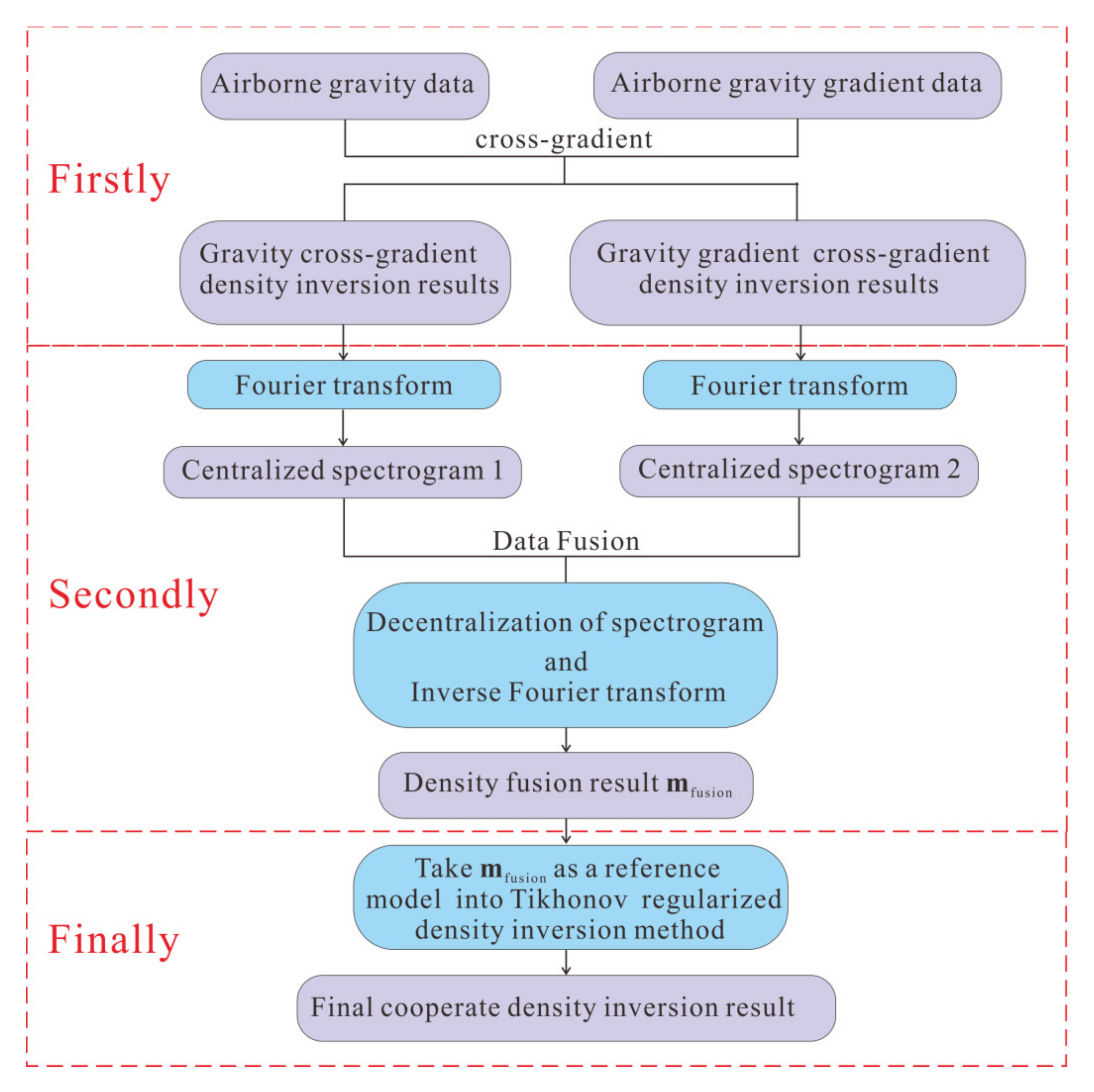
In order to improve the resolution to deep sources, we present a high-resolution cooperate density-integrated inversion method of integrated airborne gravity and its gradient data, and the specific computation processes are shown in Figure 1.

Firstly, we use the cross-gradient function to accomplish the joint inversion of airborne gravity and its gradient data, and this method can effectively keep the characteristics of different types of data. The cross-gradient function is mostly used for joint inversion between different physical parameters, and the cross-product of the gradient vectors of different physical parameters is used to reflect the structural similarity of the target body. The cross-gradient term is introduced into the inversion objective function to achieve structural constraints. So, the inversion result computed by the cross-gradient method is more convergent. The cross-gradient function of the two physical parameters m⁽¹⁾ and m⁽²⁾ are defined as follows [49,50]

$${\mathrm{\Phi }}_{\mathrm{cross}}({\mathit{m}}^{(1)},{\mathit{m}}^{(2)})=\nabla {\mathit{m}}^{(1)}(x,y,z)\times \nabla {\mathit{m}}^{(2)}(x,y,z)=(t_x,t_y,t_z),$$

(6)

$$t_x({\mathit{m}}^{(1)},{\mathit{m}}^{(2)})=\frac{\partial {\mathit{m}}^{(2)}(y,z)}{\partial y}\frac{\partial {\mathit{m}}^{(1)}(y,z)}{\partial z}-\frac{\partial {\mathit{m}}^{(1)}(y,z)}{\partial y}\frac{\partial {\mathit{m}}^{(2)}(y,z)}{\partial z},$$

(7)

$$t_y({\mathit{m}}^{(1)},{\mathit{m}}^{(2)})=\frac{\partial {\mathit{m}}^{(2)}(x,z)}{\partial z}\frac{\partial {\mathit{m}}^{(1)}(x,z)}{\partial x}-\frac{\partial {\mathit{m}}^{(1)}(x,z)}{\partial z}\frac{\partial {\mathit{m}}^{(2)}(x,z)}{\partial x},$$

(8)

$$t_z({\mathit{m}}^{(1)},{\mathit{m}}^{(2)})=\frac{\partial {\mathit{m}}^{(2)}(x,y)}{\partial x}\frac{\partial {\mathit{m}}^{(1)}(x,y)}{\partial y}-\frac{\partial {\mathit{m}}^{(1)}(x,y)}{\partial x}\frac{\partial {\mathit{m}}^{(2)}(x,y)}{\partial y},$$

(9)

where m⁽¹⁾ and m⁽²⁾ represent the gradient of two physical parameters.

Although the airborne gravity and its gradient data both reflect the density change, the characteristics of the two data are different. The cross-gradient constraint function is considered for structural constraints to achieve joint inversion of different forms of data under the same physical property. The objective functions of airborne gravity and its vertical gradient cross-gradient inversion are as follows

$$\mathrm{\Phi }({\mathit{m}}^{(1)},{\mathit{m}}^{(2)})={‖{\mathit{W}}_{\mathrm{d}}\left[\begin{array}{c}{\mathit{G}}^{(1)}{\mathit{m}}^{(1)}-{\mathit{d}}^{(1)}\\ {\mathit{G}}^{(2)}{\mathit{m}}^{(2)}-{\mathit{d}}^{(2)}\end{array}\right]‖}_2^2+\alpha {‖{\mathit{W}}_{\mathrm{m}}\left[\begin{array}{c}({\mathit{m}}^{(1)}-{\mathit{m}}_0{}^{(1)})\\ ({\mathit{m}}^{(2)}-{\mathit{m}}_0{}^{(2)})\end{array}\right]‖}_2^2+\lambda {‖{\mathrm{\Phi }}_{\mathrm{cross}}({\mathit{m}}^{(1)},{\mathit{m}}^{(2)})‖}_2^2$$

(10)

where G⁽¹⁾ and G⁽²⁾ represent the kernel function matrices corresponding to airborne gravity data and its gradient data, respectively. m⁽¹⁾ and m⁽²⁾ represent the density parameters corresponding to airborne gravity data and its gradient data, respectively. d⁽¹⁾ and d⁽²⁾ represent gravity anomaly and its gradient anomaly. W_d is the data-weighting matrix. α is the regularization coefficient that is optimized at each iteration to minimize the error weighted root mean square error. λ is the coefficient of the cross-gradient terms. The amount of structural similarity obtained through the joint inversion algorithm can be adjusted using different choices of λ [51]. At each iteration k, the parameter λ is reduced slowly dependent on parameter γ, using λ^(k) = λ^(k−1)γ, where 0 ≤ γ < 1. The cross-gradient method can effectively reflect the features that the original airborne gravity data are sensitive to deep sources, and the airborne gravity gradient data can highlight the shallow sources.

Secondly, we merge two different density results computed by the cross-gradient method into a result under the condition of keeping the characteristic of different results, and the Fourier and wavelet transforms are two commonly used fusion methods [52,53]. The different wavelet decomposition orders will affect the fusion results, and it is hard to ascertain the reasonable order for real data, so we adopt the Fourier transform fusion method, and the expression is

$$\mathit{G}(\mathit{\omega })={\mathit{F}}_{{\mathrm{g}}_{\mathrm{z}}}(\mathit{\omega }){\mathit{H}}_{\mathrm{lowpass}}+{\mathit{F}}_{{\mathrm{g}}_{\mathrm{zz}}}(\mathit{\omega })(1-{\mathit{H}}_{\mathrm{lowpass}}),$$

(11)

$${\mathit{m}}_{\mathrm{fusion}}={\mathit{F}}^{-1}\mathit{G}(\mathit{\omega }),$$

(12)

where $\mathit{F}$ represents Fourier transform, ${\mathit{F}}^{-1}$ represents inverse Fourier transform. ${\mathit{F}}_{\mathrm{g}}(\mathit{\omega })$ and ${\mathit{F}}_{{\mathrm{g}}_{\mathrm{zz}}}(\mathit{\omega })$ are the airborne gravity data, and its gradient data in the frequency domain after Fourier transform, and ${\mathit{H}}_{\mathrm{lowpass}}$ represents the low pass filter, which remains the low-frequency information of gravity data.

Finally, we take the fusion results m_fusion as the reference model and use the format of the Tikhonov regularized density inversion method to obtain the final density result by the combination of airborne gravity and its gradient data, and the computation process solved by the conjugate gradient algorithm is

• k = 0, ${\mathit{m}}_0={\mathit{m}}_{\mathrm{fusion}}$
• ${\mathit{d}}_{\mathrm{k}}=\mathit{G}{\mathit{m}}_{\mathrm{k}}$, $\mathsf{\Delta }\mathit{d}=\mathit{d}-{\mathit{d}}_{\mathrm{k}}$. (k = 0,1,2…)
• $\mathsf{\Delta }\mathit{m}={({\mathit{G}}^{\mathrm{T}}\mathit{G}+\lambda {\mathit{W}}_{\mathrm{m}})}^{-1}{\mathit{G}}^{\mathrm{T}}\mathsf{\Delta }\mathit{d}$
• ${\mathit{m}}_{\mathrm{k}+1}={\mathit{m}}_{\mathrm{k}}+\mathsf{\Delta }\mathit{m}$

where $\mathit{G}={\left[{\mathit{G}}_{\mathrm{z}};{\mathit{G}}_{\mathrm{xx}};{\mathit{G}}_{\mathrm{xy}};{\mathit{G}}_{\mathrm{xz}};{\mathit{G}}_{\mathrm{yz}};{\mathit{G}}_{\mathrm{zz}}\right]}^{\mathrm{T}}$, $\mathit{d}={\left[{\mathit{d}}_{\mathrm{z}};{\mathit{d}}_{\mathrm{xx}};{\mathit{d}}_{\mathrm{xy}};{\mathit{d}}_{\mathrm{xz}};{\mathit{d}}_{\mathrm{yz}};{\mathit{d}}_{\mathrm{zz}}\right]}^{\mathrm{T}}$. k is the number of iteration, and k = 0 means the initial condition, and the iteration termination condition is that data fitting error is less than the given threshold.

3. Theoretical Model Tests

Airborne gravity gradiometry data has a higher horizontal resolution to shallower causative sources than airborne gravity anomaly, so joint exploration of airborne gravity and its gradient data can simultaneously obtain the anomaly feature of sources with different depths. In order to verify the effectiveness of the high-resolution cooperate density-integrated inversion method, we build models of two prisms in different depths with the density contrast of 1000 kg/m^3, which have depths from 2 to 4 km and 4 to 7 km, and sizes of models are 2 × 2 × 2 km and 4 × 2 × 3 km, as shown in Figure 2a.

Compared with Figure 2b,c, airborne gravity gradiometry data better highlight shallow information than airborne gravity anomaly, and airborne gravity data better displays deep information.

To verify the high-resolution results of the proposed cooperate density-integrated inversion method, we come up with the density results by common Tikhonov regularized method, data combined joint inversion method, structure constrained joint inversion method, and cooperate density-integrated inversion method. The subsurface is divided into 30 × 20 × 10 cubic prisms with an edge length of 1 km.

Figure 3a shows the density inversion result of gravity anomaly by common Tikhonov regularized method with y-slice of 10 km, and the results have a lower resolution to the shallower body. The root mean square misfit of data is 0.15. Figure 3b represents the density result of airborne gravity gradient data by Tikhonov regularized inversion method with y-slice of 10 km, which can clearly show the location of the shallow source. The root mean square misfit of data is 0.01. Figure 3c,d shows the density slice and 3D density distribution by data combined joint inversion method of airborne gravity and its gradient data. The root mean square misfit of data is 0.008. We find that the joint inversion improves the resolution and accuracy of the shallow source, but it has a lower resolution to the deep source. Figure 3e,f show the density inversion results of airborne gravity and gradient data computed by structure constrained joint inversion method, respectively, and it can recover a more compact model than separate inversion. The root mean square misfits of data are 0.004 and 0.002. The cooperate density-integrated inversion method is introduced and combined with the advantages of the results by different data, the vertical slice and 3D perspective view with a value larger than 350 kg/m³ are shown in Figure 3g,h, and we obviously find that the shape of recovered density models is refined. The root mean square misfit of data is 0.001. It is proved that the cooperate density-integrated inversion method of airborne gravity and its gradient data have a higher horizontal and vertical resolution that is more convergent compared to the data combined joint inversion method.

During the density inversion, the existence of noise will have a great impact on the inversion results, and noise is inevitable in actual situations. To test the anti-noisy of the high-resolution cooperate density-integrated inversion method and simulate the actual noise condition, we build the same model contaminated by 5% Gaussian noise in Figure 2a. Figure 4b displays noise-corrupted airborne gravity anomaly and its gradient anomaly, and the noise has an obvious impact on the anomaly shape.

The airborne gravity and its gradient data are affected by noise. The density result with a slice of y = 10 km computed by the data combined joint inversion method is distorted, as shown in Figure 5a. So, the 3D density distribution with larger than 350 kg/m³ cannot obtain the results with high resolution. Figure 5c,d show the density results with a slice of y = 10 km and the 3D density distribution with larger than 350 kg/m³ computed by the presented cooperative inversion method. Although the airborne gravity and its vertical gradient data are affected by noise, the density results obtained by the presented cooperative inversion method can obtain better recovery of physical parameters and more accurate position descriptions.

For testing the universality of the proposed method, we build models with two prisms buried at the same depth, and the density contrast of the prism is 1000 kg/m^3, which have depths from 2 to 4 km, and the size of models are 4 × 2 × 2 km and 4 × 2 × 2 km, as shown in Figure 6a. The airborne gravity anomaly and gravity gradient anomaly are as shown in Figure 6b,c.

Previous studies have shown that a gradiometer is better than a gravimeter in detecting short-wavelength anomalies at the same depth [54]. For the models buried at the same depth, airborne gravity gradiometry data achieve a more detailed description and a better description of the shape of target bodies compared to the airborne gravity data. The subsurface is divided into 20 × 20 × 10 cubic prisms with an edge length of 1 km.

We obtain the density results with a slice of y = 10 km and the 3D density distribution with larger than 370 kg/m³ computed by the data combined joint inversion method as shown in Figure 7a,b. The density results are not focused enough and cannot describe the distribution of models clearly. The density results with a slice of y = 10 km and the 3D density distribution larger than 370 kg/m³ computed by the presented cooperate density-integrated inversion method are shown in Figure 7c,d. Compared to the density results computed by the data combined joint inversion method, the results computed by the presented cooperative inversion method are more convergent, and both horizontal and vertical resolution is higher, and the density distributions are closer to the true value. So, the presented cooperative inversion method can obtain high-resolution results for the models buried at the same depth.

In actual situations, the distributions of iron mines are complex. To verify the acceptability of the proposed method under the actual situation, we build complex models with three prisms, and the density contrasts of the prisms are 800, 1000, and 1200 kg/m^3, which have depths from 2 to 4 km, 4 to 7 km, and 2 to 4 km, as shown in Figure 8a, and the sizes of models are 4 × 4 × 2 km, 6 × 2 × 3 km, and 4 × 4 × 2 km. The airborne gravity anomaly and gravity gradient anomaly are as shown in Figure 8b,c.

Also, the subsurface is divided into 40 × 20 × 10 cubic prisms with an edge length of 1 km.

The density results with a slice of x = 10 km and y = 10 km computed by the data combined joint inversion method as shown in Figure 9a,c, and the black lines represent the true distribution of sources. The results can obtain better recovery of physical parameters to shallower causative sources. However, the results cannot obtain a suitable description of deep causative sources. The density results with a slice of x = 10 km and y = 10 km computed by the presented cooperative inversion method are shown in Figure 9b,d. The 3D density distributions with larger than 370 kg/m³ computed by the data combined joint inversion method and the presented cooperative inversion method are shown in Figure 9e,f. The results computed by the presented cooperative inversion method have a higher horizontal and vertical resolution, which is more convergent compared to the current inversion method, and the density distributions are closer to the true value. So, the presented cooperative inversion method can obtain high-resolution results for the complex model tests.

To test the accuracy of the proposed cooperate density-integrated inversion method depends upon the airborne’s height, we build the same complex model in Figure 10a. With the airborne’s height increase, the maximum of gravity and its vertical gradient data reduce significantly, and the characteristics are very different from the form in Figure 10b,c.

For density inversion results calculated at 150 m altitude, the recovery of the shallow bodies is missing, as shown in Figure 10c,d, and the deep body is out of convergence. Figure 10g,h are density slice (y = 10 km) by cooperate density-integrated inversion method at 200 m altitude and 3D density distribution (larger than 370 kg/m³). For density inversion results calculated at 200 m altitude, it is far from the real model. So, with the increase in altitude, it has a great influence on the final inversion results, and the results are more deviated from the real model.

When the airborne gravity gradient data are not measured, as an alternative, the airborne gravity vertical gradient data can be calculated from airborne gravity data, and we calculate airborne gravity vertical gradient data by Fourier transform method. In order to verify the feasibility of this method, we carried out the following work. Firstly, we compare the calculated airborne gravity gradient data and theoretical airborne gravity gradient data (Figure 8c). Then, we obtain the density slice by cooperate density-integrated inversion method of airborne gravity and its calculated vertical gradient data. Finally, we achieve the 3D density distribution (larger than 370 kg/m³) by cooperate density-integrated inversion method.

We find that the theoretical airborne gravity gradient data (Figure 8c) and calculated airborne gravity gradient data (Figure 11a) are almost the same. The density results (Figure 11b) with a slice of y = 10 km computed by the proposed cooperate density-integrated inversion method are close to the same results in Figure 9d. Three-dimensional density distributions (Figure 11c) with larger than 370 kg/m³ computed by the presented cooperative inversion method are consistent with the same distribution in Figure 9f. Compared with the results, we confirm that the calculated vertical gradient data is also available when missing the real gravity gradient data, and the inversion results by cooperate density-integrated inversion method are almost the same. So, we can use the calculated gravity gradient data to replace the real gravity gradient data under the condition of missing data.

4. Real Data Application

The western Liaoning Province is rich in iron ore bodies, which shows the high value of airborne gravity anomaly. In order to obtain the clear distribution of the mineral-induced anomalous source, we use the joint exploration of airborne gravity and its vertical gradient data with a sampling interval of 250 m, and the vertical gradient data are obtained by calculating the vertical derivative of gravity data. The geological map is shown in Figure 12a, and the distributions of the iron mines are predicted by the regional structural feature, and both fault and Quaternary coverage areas are identified by geological information [55,56]. The airborne gravity anomaly and its vertical gradient anomaly are shown in Figure 12b,c, and there is a suitable corresponding relationship between the high values of anomalies and the predicted locations of iron mine, and the gravity gradient data has a higher resolution. Based on the drilling data W1 as shown in Figure 12d, we can verify the accuracy of the inversion results, and the drilling data also provide the accurate density contrast for obtaining the delineation of iron ore bodies.

Through the demonstration in Figure 11, calculated gravity gradient data can replace the actual gravity gradient data, and the inversion result can obtain high-resolution and accurate results by the proposed cooperate density-integrated inversion method. Density inversion results are carried out for airborne gravity data, and its calculated vertical gradient data in the western Liaoning area by data combined joint inversion method and the proposed cooperate density-integrated inversion method. There has a drilled borehole in the survey area, and the borehole is located inside the high-value area. Based on the drilling data W1, the high-density magnetite ore bodies are almost 3120 kg/m³, and surrounding skarn are almost 2900 kg/m³. It is believed that high-density bodies that are greater than or equal to 200 kg/m³ correspond well to the range of iron mines. So, we retain density bodies with a value greater than 200 kg/m³, as shown in Figure 13a,c.

In order to confirm the buried depth of the density results, we obtain the horizontal slices of 3D density results by data combined joint inversion method from 0 to 1500 m as shown in Figure 13b and obtain the horizontal slices of 3D density results by proposed cooperative density inversion method from 0 to 1500 m as shown in Figure 13d. We estimate that the high-density bodies were buried from 900 to 1300 m.

According to the cooperative density inversion result, we delineate the horizontal range of high-density bodies, as shown in Figure 14. Compared to the inferred range of iron mines by geological information, the density inversion result by the proposed cooperative method has a better agreement than the density by data combined joint inversion method. Therefore, cooperate density-integrated inversion method has the ability to achieve higher resolution density inversion result by gravity data and its gradient data, and the proposed method presents more detailed features compared to the geological results.

Figure 14b displays that the results computed by the proposed method are more accurate and have higher resolution and more specific detailed descriptions of the iron bodies. Finally, we identify five iron mines depending on the inversion results of the proposed method, named I–V. The buried depth ranges of the five iron bodies are determined according to the two profiles. The buried depth of the iron mine area I is 900–1300 m. The buried depth of the iron mine area II is 1000–1100 m, the iron mine area III is 900–1200 m, the iron mine area IV is 950–1200 m, and the iron mine area V is 1000–1200 m.

5. Conclusions

We propose a cooperate density-integrated inversion method of airborne gravity and its gradient data, which used the cross-gradient and fusion tools to obtain higher resolution results, especially that the proposed method can better obtain the distribution of the deep source. We tested the proposed method by synthetic model tests and real data. Both model tests verified that the cooperate density-integrated inversion method of airborne gravity and its gradient data can obtain high-resolution results, which are buried at the same depth and different depths. Moreover, inversion results of complex models showed the feasibility of the proposed method. This method could recover higher resolution density models compared to the data combined joint inversion. In practice, calculated airborne gravity vertical gradient data can replace the theoretical airborne gravity vertical gradient data when the airborne gravity gradient data are not measured.

The inversion results of real data provide the location of the mining area accurately and delineate five iron ore bodies buried from 900 to 1300 m. The cooperate density-integrated inversion method provides a better tool to obtain high-resolution density distribution of airborne gravity and its gradient data.

References

1. Li, Y.G.; Oldenburg, D.W. 3-D inversion of gravity data. Geophysics 1998, 2, 109–119. [Google Scholar] [CrossRef]
2. Portniaguine, O.; Zhdanov, M.S. Focusing geophysical inversion images. Geophysics 1999, 6, 874–887. [Google Scholar] [CrossRef] [Green Version]
3. Li, Y.G.; Oldenburg, D.W. Incorporating geological dip information into geophysical inversions. Geophysics 2000, 2, 148–157. [Google Scholar] [CrossRef] [Green Version]
4. Chasseriau, P.; Chouteau, M. 3D gravity inversion using a model of parameter covariance. J. Appl. Geophys. 2003, 6, 59–74. [Google Scholar] [CrossRef]
5. Zhdanov, M.S.; Ellis, R.; Mukherjee, S. Three-dimensional regularized focusing inversion of gravity gradient tensor component data. Geophysics 2004, 7, 877–1103. [Google Scholar] [CrossRef]
6. Commer, M. Three-dimensional gravity modelling and focusing inversion using rectangular meshes. Geophys. Prospect. 2011, 9, 59. [Google Scholar] [CrossRef]
7. Ghalehnoee, M.H.; Ansari, A.; Ghorbani, A. Improving compact gravity inversion using new weighting functions. Geophys. J. Int. 2017, 1, 546–560. [Google Scholar] [CrossRef]
8. Geng, M.X.; Hu, X.Y.; Zhang, H.L.; Liu, S. 3D inversion of potential field data using a marginalizing probabilistic method. Geophysics 2018, 10, G93–G106. [Google Scholar] [CrossRef]
9. Meng, Z.H.; Li, F.T. Comment on: “Fast 3D inversion of gravity data using solution space priorconditioned Lanczos bidiagonalization”, by Mohammad Rezaie, Ail Moradzadeh and Ali Nejati Kalateh. J. Appl. Geophys. 2020, 12, 42–50. [Google Scholar] [CrossRef]
10. Barnes, G.; Lumley, J. Processing gravity gradient data. Geophysics 2011, 3, I33–I47. [Google Scholar] [CrossRef]
11. Chen, T.; Yang, D.K. Gravity gradient tensors derived from radial component of gravity vector using taylor series expansion. Geophys. J. Int. 2021, 8, 412–431. [Google Scholar] [CrossRef]
12. Dai, C.L.; Shum, C.K.; Wang, R.J.; Wang, L. Improved constraints on seismic source parameters of the 2011 Tohoku earthquake from GRACE gravity and gravity gradient changes. Geophys. Res. Lett. 2014, 3, 1929–1936. [Google Scholar] [CrossRef] [Green Version]
13. Gao, D.Y.; Hu, B.Q.; Chang, L.B.; Qin, F.J.; Lyu, X. An Aided Navigation Method Based on Strapdown Gravity Gradiometer. Sensors 2021, 1, 829. [Google Scholar] [CrossRef]
14. Cattin, R.; Berthet, T.; Hetényi, G.; Saraswati, A.; Panet, I.; Mazzotti, S.; Cadio, C.; Ferry, M. Joint inversion of ground gravity data and satellite gravity gradients between Nepal and Bhutan: New insights on structural and seismic segmentation of the Himalayan arc. Phys. Chem. Earth 2021, 10, 103002. [Google Scholar] [CrossRef]
15. Plasman, M.; Tiberi, C.; Cadio, C.; Saraswati, A.T.; Pajot-Métivier, G.; Diament, M. From space to lithosphere: Inversion of the GOCE gravity gradients. Supply to the Earth’s interior study. Geophys. J. Int. 2020, 6, 398–419. [Google Scholar] [CrossRef]
16. Dransfield, M.; Zeng, Y. Airborne gravity gradiometry terrain correction and elevation error. Geophysics 2009, 9, I37–I42. [Google Scholar] [CrossRef]
17. Kass, M.; Li, Y. Practical aspects of terrain correction in airborne gravity gradiometry surveys. Explor. Geophys. 2007, 9, 198–203. [Google Scholar] [CrossRef]
18. Eppelbaum, L.V. Geophysical potential fields: Geological and environmental applications. In Computational Geophysics; Elsevier: Amsterdam, The Netherlands, 2019; p. 7. [Google Scholar]
19. Bell, R.E.; Anderson, R.; Pratson, L. Gravity gradiometry resurfaces. Lead. Edge 1997, 1, 55–59. [Google Scholar] [CrossRef] [Green Version]
20. Fedi, M.; Hansen, P.C.; Paoletti, V. Analysis of depth resolution in potential-field inversion. Digit. Libr. Home 2005, 11, A1–A11. [Google Scholar] [CrossRef]
21. Droujinine, A.; Vasilevsky, A.; Evans, R. Feasibility of using full tensor gradient (FTG) data for detection of local lateral density contrasts during reservoir monitoring. Geophys. J. Int. 2007, 6, 795–820. [Google Scholar] [CrossRef] [Green Version]
22. Difrancesco, D.; Grierson, A.; Kaputa, D.; Meyer, T. Gravity gradiometer systems—Advances and challenges. Geophys. Prospect. 2009, 6, 615–623. [Google Scholar] [CrossRef]
23. Vasco, D.W. Resolution and variance operators of gravity and gravity gradiometry. Geophysics 2012, 7, 889–899. [Google Scholar] [CrossRef]
24. Meju, M.A.; Gallardo, L.A.; Mohamed, A. Evidence for correlation of electrical resistivity and seismic velocity in heterogeneous near-surface materials. Geophys. Res. Lett. 2003, 4, 1373. [Google Scholar] [CrossRef]
25. Gallardo, L.A. Multiple cross-gradient joint inversion for geospectral imaging. Geophys. Res. Lett. 2007, 10, L19301. [Google Scholar] [CrossRef]
26. Fregoso, E.; Gallardo, L.A. Cross-gradients joint 3D inversion with applications to gravity and magnetic data. Geophysics 2009, 7, L31. [Google Scholar] [CrossRef]
27. Farshad, J.; Ali, M.; Faramarz, D.A. An Improved 3D Joint Inversion Method of Potential Field Data Using Cross-Gradient Constraint and LSQR Method. Pure Appl. Geophys. 2018, 12, 4389–4409. [Google Scholar] [CrossRef]
28. Max, M.; Björn, H.; Marion, J.; Alan, W.R.; Richard, W.H. A framework for 3-D joint inversion of MT, gravity and seismic refraction data. Geophys. J. Int. 2011, 1, 477–493. [Google Scholar] [CrossRef]
29. Gallardo, L.A.; Meju, M.A. Structure-coupled multiphysics imaging in geophysical sciences. Rev. Geophys. 2011, 3, 1–19. [Google Scholar] [CrossRef]
30. Zhang, R.Z.; Li, T.L.; Deng, X.H.; Huang, X.G.; Pak, Y. Two-dimensional data-space joint inversion of magnetotelluric, gravity, magnetic and seismic data with cross-gradient constraints. Geophys. Prospect. 2020, 2, 721–731. [Google Scholar] [CrossRef]
31. Jiang, W.B. 3-D joint inversion of seismic waveform and airborne gravity gradiometry data. Geophys. J. Int. 2020, 223, 746–764. [Google Scholar] [CrossRef]
32. Wu, L.; Ke, X.P.; Hsu, H.; Fang, J.; Xiong, C.Y.; Wang, Y. Joint gravity and gravity gradient inversion for subsurface object detection. IEEE Geoence. Remote Sens. Lett. 2013, 7, 865–869. [Google Scholar] [CrossRef]
33. Wan, L.; Zhdanov, M.S. Iterative migration of gravity and gravity gradiometry data. In SEG Technical Program Expanded Abstracts; Society of Exploration Geophysicists: Houston, TX, USA, 2013; pp. 1211–1215. [Google Scholar]
34. Capriotti, J.; Li, Y.G. Gravity and gravity gradient data: Understanding their information content through joint inversions. In SEG Technical Program Expanded Abstracts; Society of Exploration Geophysicists: Houston, TX, USA, 2014; p. 1949. [Google Scholar]
35. Zhdanov, M.S.; Lin, W. Adaptive multinary inversion of gravity and gravity gradient data. Geophysics 2017, 11, G101–G114. [Google Scholar] [CrossRef]
36. Liu, J.Z.; Liu, L.T.; Liang, X.H.; Ye, Z.R. 3D density inversion of gravity gradient data using the extrapolated tikhonov regularization. Appl. Geophys. 2015, 6, 137–146. [Google Scholar] [CrossRef]
37. Ranchin, T.; Wald, L. The wavelet transform for the analysis of remotely sensed images. Int. J. Remote. Sens. 1993, 10, 615–619. [Google Scholar] [CrossRef]
38. Douma, H.; De Hoop, M.V. Leading-order seismic imaging using curvelets. Geophysics 2007, 12, S231–S248. [Google Scholar] [CrossRef] [Green Version]
39. Herrmann, F.J.; Wang, D.L.; Hennenfent, G.; Moghaddam, P.P. Curvelet-based seismic data processing: A multiscale and nonlinear approach. Geophysics 2007, 12, A1–A5. [Google Scholar] [CrossRef]
40. Candes, E.J.; Donoho, D. Continuous curvelet transform: II. Discretization and frames. Appl. Comput. Ilarmoncc Anal. 2005, 9, 198–222. [Google Scholar] [CrossRef] [Green Version]
41. Nencinia, F.; Garzeli, A.; Baronti, S.; Alparone, L. Remote sensing image fusion using the curvelet transform. Inf. Fusion 2007, 4, 143–156. [Google Scholar] [CrossRef]
42. Huang, M.T.; Ouyang, Y.Z.; Zhai, G.J.; Deng, K.L.; Lu, X.P.; Wu, T.Q. Tikhonov Regularization Collocation for Multi-source Gravity Data Fusion Processing. Hydrogr. Surv. Charting 2013, 5, 6–12. [Google Scholar] [CrossRef]
43. Tikhonov, A.N.; Arsenin, V.Y. Solusions of Ill-Posed Problems; John Wiley and Sons Inc.: New York, NY, USA, 1977; p. 5. [Google Scholar]
44. Vatankhah, S.; Ardestani, V.E.; Renaut, R.A. Automatic estimation of the regularization parameter in 2D focusing gravity inversion: Application of the method to the safo manganese mine in the northwest of iran. J. Geophys. Eng. 2014, 1, 4. [Google Scholar] [CrossRef] [Green Version]
45. Farquharson, C.G.; Oldenburg, D.W. A comparison of automatic techniques for estimating the regularization parameter in non-linear inverse problems. Geophys. J. Int. 2004, 3, 411–425. [Google Scholar] [CrossRef] [Green Version]
46. Li, Y.G.; Oldenburg, D.W. 3D inversion of magnetic data. Geophysics 1996, 4, 394–408. [Google Scholar] [CrossRef]
47. Portniaguine, O.; Zhdanov, M.S. 3-D magnetic inversion with data compression and image focusing. Geophysics 2002, 67, 1532–1541. [Google Scholar] [CrossRef] [Green Version]
48. Gao, X.H.; Xiong, S.Q.; Yu, C.C.; Zhang, D.S.; Wu, C.P. The Estimation of Magnetite Prospective Resources Based on Aeromagnetic Data: A Case Study of Qihe Area, Shandong Province, China. Remote Sens. 2021, 3, 1216. [Google Scholar] [CrossRef]
49. Meju, L. Characterization of heterogeneous near-surface materials by joint 2D inversion of dc resistivity and seismic data. Geophys. Res. Lett. 2003, 7, 183–196. [Google Scholar] [CrossRef]
50. Gallardo, L.A.; Meju, M.A. Joint two-dimensional DC resistivity and seismic travel time inversion with cross-gradients constraints. J. Geophys. Res. Solid Earth 2004, 3, 109. [Google Scholar] [CrossRef]
51. Vatankhah, S.; Liu, S.; Renaut, R.A.; Hu, X.; Hogue, J.D.; Gharloghi, M. An Efficient Alternating Algorithm for the Lp-Norm Cross-Gradient Joint Inversion of Gravity and Magnetic Data Using the 2-D Fast Fourier Transform. IEEE Trans. Geosci. Remote Sens. 2020, 10, 1–16. [Google Scholar] [CrossRef]
52. Otazu, X.; Gonzalez-Audicana, M.; Fors, O.; Nunez, J. Introduction of sensor spectral response into image fusion methods. application to wavelet-based methods. IEEE Trans. Geosci. Remote Sens. 2005, 10, 2376–2385. [Google Scholar] [CrossRef] [Green Version]
53. Ghellab, A.M.R.; Belbachir, M.F. Efficient image fusion method based on the fourier transform by introducing sensor spectral response. J. Appl. Remote Sens. 2013, 5, 073552. [Google Scholar] [CrossRef]
54. Beiki, M.; Pedersen, L.B. Eigenvector analysis of gravity gradient tensor to locate geologic bodies. Geophysics 2010, 10, I37–I49. [Google Scholar] [CrossRef]
55. Jia, B.; Ding, Q.H.; Yang, W.H.; Zhang, C.H.; Guo, S.Z. Evolusion of sihetuen-houyanzigou early cretaceous volcanic cluster apparatus and volcanic effusive activity in western Liaoning. Acta Petrol. Sin. 2009, 5, 1191–1200. [Google Scholar] [CrossRef]
56. Yin, J.N.; Mark, L.; Teng, S.R. Mineral prospectivity analysis for BIF iron deposits: A case study in the Anshan-Benxi area, Liaoning province, North-East China—ScienceDirect. Ore Geol. Rev. 2018, 11, 2376–2385. [Google Scholar] [CrossRef]
Figure 1. Flowchart of the cooperate density-integrated inversion method.
Remotesensing 13 04157 g001
Figure 2. Information of models in different depth. (a) Density models with 1000 kg/m3. (b) Airborne gravity anomaly at 100 m altitude. (c) Vertical gradient anomaly of airborne gravity data at 100 m altitude.
Remotesensing 13 04157 g002
Figure 3. Model tests of two prisms in different depths. (a) Density slice (y = 10 km) by Tikhonov regularized method of airborne gravity data. (b) Density slice (y = 10 km) by Tikhonov regularized method of airborne gravity gradient data. (c) Density slice (y = 10 km) by data combined joint inversion method of airborne gravity and its gradient data. (d) 3D density distribution (larger than 350 kg/m3) by data combined joint inversion method of airborne gravity and its gradient data. (e) Density slice (y = 10 km) by structure constrained joint inversion method of airborne gravity data. (f) Density slice (y = 10 km) by structure constrained joint inversion method of airborne gravity gradient data. (g) Density slice (y = 10 km) by cooperate density-integrated inversion method. (h) 3D density distribution (larger than 350 kg/m3) by the cooperate density-integrated inversion method.
Remotesensing 13 04157 g003aRemotesensing 13 04157 g003b
Figure 4. Information of models in different depths with 5% Gaussian noise. (a) Airborne gravity anomaly at 100 m altitude. (b) Vertical gradient anomaly of airborne gravity at 100 m altitude.
Remotesensing 13 04157 g004
Figure 5. Model tests of two prisms in different depths containing noise. (a) Density slice (y = 10 km) by data combined joint inversion method of airborne gravity and its gradient data. (b) 3D density distribution (larger than 350 kg/m3) by data combined joint inversion method of airborne gravity and its gradient data. (c) Density slice (y = 10 km) by the cooperate density-integrated inversion method. (d) 3D density distribution (larger than 350 kg/m3) by the cooperate density-integrated inversion method.
Remotesensing 13 04157 g005
Figure 6. Information of models in the same depth. (a) Density models with 1 kg/m3. (b) Airborne gravity anomaly at 100 m altitude. (c) Vertical gradient anomaly of airborne gravity data at 100 m altitude.
Remotesensing 13 04157 g006
Figure 7. Model tests of two prisms in the same depths. (a) Density slice (y = 10 km) by data combined joint inversion method of airborne gravity and its gradient data. (b) 3D density distribution (larger than 370 kg/m3) by data combined joint inversion method of airborne gravity and its gradient data. (c) Density slice (y = 10 km) by the cooperate density-integrated inversion method. (d) 3D density distribution (larger than 370 kg/m3) by the cooperate density-integrated inversion method.
Remotesensing 13 04157 g007
Figure 8. Information of complex models. (a) Density models with 1000 kg/m3. (b) Airborne gravity anomaly at 100 m altitude. (c) Vertical gradient anomaly of airborne gravity at 100 m altitude.
Remotesensing 13 04157 g008
Figure 9. Complex model tests of three prisms. (a) Density slice (x = 10 km) by data combined joint inversion method of airborne gravity and its gradient data. (b) Density slice (x = 10 km) by cooperate density-integrated inversion method. (c) Density slice (y = 10 km) by data combined joint inversion method of airborne gravity and its gradient data. (d) Density slice (y = 10 km) by the cooperate density-integrated inversion method. (e) 3D density distribution (larger than 370 kg/m3) by data combined joint inversion method of airborne gravity and its gradient data. (f) 3D density distribution (larger than 370 kg/m3) by the cooperate density-integrated inversion method of airborne gravity and its gradient data.
Remotesensing 13 04157 g009
Figure 10. Complex model tests with different altitudes. (a) Airborne gravity anomaly at 150 m altitude. (b) Vertical gradient anomaly of airborne gravity at 150 m altitude. (c) Density slice (y = 10 km) by cooperate density-integrated inversion method at 150 m altitude. (d) 3D density distribution (larger than 370 kg/m3). (e) Airborne gravity anomaly at 200 m altitude. (f) Vertical gradient anomaly of airborne gravity at 200 m altitude. (g) Density slice (y = 10 km) by cooperate density-integrated inversion method at 200 m altitude. (h) 3D density distribution (larger than 370 kg/m3).
Remotesensing 13 04157 g010
Figure 11. Complex model tests using airborne gravity and calculated vertical gradient data. (a) Calculated airborne gravity gradient data. (b) Density slice (y = 10 km) by cooperate density-integrated inversion method. (c) 3D density distribution (larger than 370 kg/m3) by cooperate density-integrated inversion method.
Remotesensing 13 04157 g011aRemotesensing 13 04157 g011b
Figure 12. Real data. (a) Geological map of Liaoning western area. (b) Real airborne gravity anomaly of Liaoning western area. (c) Calculated airborne gravity vertical gradient anomaly of Liaoning western area. (d) Drilling data information.
Remotesensing 13 04157 g012aRemotesensing 13 04157 g012b
Figure 13. Density inversion result of real data. (a) The vertical slices and the 3D density results with the value larger than 0.2 kg/m3 computed by data combined joint inversion method. (b) The horizontal slices of 3D density results computed by the data combined joint inversion method. (c) The vertical slices and the 3D density results with a value larger than 0.2 kg/m3 computed by the proposed cooperative density inversion method. (d) The horizontal slices of 3D density results computed by the proposed cooperative density inversion method.
Remotesensing 13 04157 g013
Figure 14. Distribution of density inversion results. (a) The modified location of iron mines by data combined joint inversion method. (b) The modified location of iron mines by the proposed cooperative density inversion method.
Remotesensing 13 04157 g014
Publisher’s Note: MDPI stays neutral with regard to jurisdictional claims in published maps and institutional affiliations.