Features of Winter Stratosphere Small-Scale Disturbance during Sudden Stratospheric Warmings

Abstract

We analyzed the characteristics of small-scale wave disturbances emerging during the evolution and transformation of the jet stream (JS) in the winter stratosphere and the lower mesosphere of the northern hemisphere, including the periods of sudden stratospheric warming (SSW) events. Continuous generation of small-scale wave disturbances is shown to occur over quiet geomagnetic winter periods in the region of a steady jet stream in the strato–mesosphere. We studied spatial spectra for the vertical velocity variations, determined by the parameters of emerging wave disturbances. The greatest intensities of disturbances are recorded in the regions corresponding to the high velocities of the JS (from 100 m/s and higher). In the northern hemisphere, those latitudes encompass ~40–60° N. When a steady jet stream forms, the horizontal length and periods of the most intensive wavelike disturbances are shown to vary within 300–1000 km and 50–150 min correspondingly (which match the characteristic scales of internal gravity waves, or IGWs). During the SSW prewarming stage, the JS transforms substantially. Over the same periods, a disturbance intensification is recorded, as well as the emergence of larger-scale disturbances with 3000–5000-km horizontal wavelengths, and even higher. After the SSW peak and during the stratosphere circulation recovery, the velocity in the JS substantially decreases and an essential reduction in wave-disturbance generation occurs. There are decreases in the average amplitude values (by factors of 1.8–6.7). The strongest amplitude drop was observed for short waves (zonal wavelength λ_U = 300 km). The maximum attenuation for all wavelengths was observed for the strongest 2008/2009 winter SSW. For the analyzed events, such attenuation was observed for up to about a month after the SSW peak. Thus, JS disruption during major SSWs leads to deactivating the source for generating small-scale wave disturbances in the stratosphere. This may affect disturbances in higher atmospheric layers. The results obtained are the experimental evidence that JS itself is the primary source for the generation of IGWs in the stratosphere–lower mesosphere.

1. Introduction

1.1. Winter Circumpolar Vortex and a Jet Stream

Some of the characteristic features of the stratospheric circulation at the near-polar latitudes are seasonal formation, evolution, and decay of an intensive cyclonic vortex. Under the polar night conditions, the high latitude atmosphere (under the quiet helio-geomagnetic state) is completely cut off from the solar source of thermal energy. Global circulation is determined by a stationary geostrophic current directed from west to east (the so-called western transport), which forms a circumpolar vortex (CPV) [1,2,3]. The circumpolar vortex represents a cyclonic circulation that forms in a cold air mass over the polar region and encompasses the upper stratosphere and the lower mesosphere. The CPV features an evolution of the jet stream (JS)—a narrow, spatially-limited flux of atmospheric gas with an almost horizontal axis, high velocity, and large vertical and horizontal wind shears. The motion of air mass in a jet stream occurs at a high velocity (up to 100 m/s and higher), west-to-east, and the air temperature in the stratosphere is low (200 °K and below). The emergence of the winter stratospheric JS at the polar night boundary is elucidated by a temperature gradient that forms as a result of differences in the net radiation inside and outside the near-polar region during the winter. The more differences in the temperatures, the stronger the pressure gradients and, hence, the higher the JS velocities. The formed winter circumpolar vortex with a jet stream contrasts strikingly with much weaker easterly winds in the summer stratosphere. In both hemispheres, the CPV formation starts in the autumn, when solar heating ceases in the polar regions, and its decay occurs by late winter/early spring with the solar heating resumption in the polar regions [1,2,3,4,5].

Investigations into the CPV structure and dynamics have provoked great scientific interest [6,7]. The urgency of studying the CPV is also caused by the effect of vortices on the tropospheric weather and climate [8,9,10,11]. There are two separate planetary-scale circumpolar vortices: one in the stratosphere and the other in the troposphere [12]. Both vortices can play a role in extreme weather events, but the tropospheric one influences more crucially.

The main cause of the circumpolar vortex disturbances leading to CPV global transformations is thought to be planetary Rossby waves. The waves are generated in the northern hemisphere more effectively [13] due to orography features. In the winter, when the vortex with the western winds forms in the stratosphere, favorable conditions emerge for large-scale planetary waves to propagate from the troposphere into the stratosphere. At stratospheric heights, those waves interact with a prevalent zonal flow and disturb the stratospheric vortex. The waves break at the stratosphere vortex boundaries, which results in the emergence of the so-called surf zone [14,15]. As a result, the jet stream configuration dramatically varies during the winter, and the distribution of the jet stream key parameters (density, wind velocity, etc.) features a significant spatial inhomogeneity [1,2,3,5,7,9].

Recent experimental and model studies [16,17,18] have shown that the Arctic CPV has weakened and moved away from the North Pole towards Eurasia over the past three decades. These processes are caused by the Arctic sea ice loss (especially over the Barents-Kara Sea), enhancing planetary waves with zonal numbers 1 and 2 propagating into the stratosphere and subsequently weakening the CPV in mid-winter [16].

The winter CPV’s strongest transformation occurs during sudden stratosphere warmings [13,19]. A SSW represents an explosive temperature rise of the high-latitude stratosphere during the winter months. According to the existing notions [20], SSW events may evolve due to two reasons: an increase in the wave activity flux from the troposphere into the stratosphere (the so-called classic scenario by Matsuno [21]); and/or internal dynamical processes due to non-linear interactions of planetary waves with the mean flow at the stratospheric heights [22,23]. The result of such interactions is the CPV attenuation or even decay in the high-latitude stratosphere [24]. The JS, in this case, changes its position, while its shape is substantially modified (flattening and displacement from the pole to middle latitudes or splitting into several cyclonic and anticyclonic cells).

The warmings are attributed to major (or strong) SSWs, if besides the polar temperature increase one records a change in the mean-zonal circulation direction and in the temperature gradient over the hemisphere. The day, when a change in the zonal circulation direction occurs at 10 hPa and 60° N, is referred to as the SSW peak or central date [13]. The stratosphere return to the normal regime (the so-called recovery stage) starts after the SSW peak and advances usually more slowly than the warming evolution itself. Thus, in the winter stratosphere/lower mesosphere, during SSW events, there is a radical transformation of the polar vortex structure [13,19].

1.2. Internal Gravity Waves in a Jet Stream

In several studies, it was shown that the CPV (and the related JS) is accompanied by small-scale wave disturbances in the winter polar stratosphere and the lower mesosphere [25,26,27,28]. For example, Wu and Waters [29] produced the global maps for small-scale disturbances in the middle atmosphere at 30–80 km altitudes, related to internal gravity waves (IGW), and showed that the disturbances of horizontal scales less than ~100 km are strongly correlated with the upper-tropospheric convection, surface topography, and stratospheric jet streams. Jiang et al. [30,31], based on MLS/UARS observations, showed that the high-latitude IGWs exhibit annual variations with the peak in winter and the minimum value in the summer stratosphere. These variations in IGWs correlate with the CPV strength. Wilson et al. [32], based on the lidar observations in the south of France (44 ° N), also revealed that the maximum IGWs occurred during the winter months.

Yamashita et al. [33] studied IGW variations during the 2009 SSW in the Arctic using ECMWF-T799. The authors showed that most IGWs occur at the edge of the polar vortex, and the magnitude and occurrence of IGWs correlate with the location and strength of the polar vortex that is strongly disturbed by planetary wave growth. All IGW enhancements occur before the wind reversal; IGWs became significantly weak after the 2009 SSW. These variations are confirmed by COSMIC/GPS observations. Lidar data from the Antarctic are also used to validate IGWs as derived in ECMWF.

Schoon and Zülicke [34] developed a novel method to locally diagnose wave properties, which they termed unified wave diagnostics (UWaDi). During the 30 January 2016 minor SSW, the authors detected a local occurrence of IGWs throughout the middle atmosphere. The local wave characteristics were discussed in terms of vertical propagation. The authors detected cases with a decrease in the wave action through the tropopause up to the mid-stratosphere in contrast to a case with a strong peak in the lower stratosphere and a steady decrease above. The latter happened in an area where the wind field was affected by the minor SSW.

Shpynev et al. [35] proposed and considered, in detail, a physical mechanism for the generation of wave disturbances in the CPV. Within the polar night, a significant source of the circulation energy in the winter polar stratosphere can be the gravity potential of the cooling and downwelling stratospheric gas. The potential converts into the CPV kinetic energy. Under these conditions without sunlight and thermal energy sources, the vortex kinetic energy constantly increases due to a continuous decrease in the atmospheric gas gravitation potential. At the pressure level, the CPV has a structure similar to a swirl on the water surface. At certain critical wind velocities in the jet stream, baroclinic-type instabilities form at the boundary between gas flows with different velocities and/or directions. Such conditions, for example, arise at the boundary between a JS with high velocities and an ambient atmosphere with relatively weak winds, or at the boundary of vortices, which are formed as a result of CPV transformation during an SSW event. The instabilities produce atmospheric waves of various scales, including IGWs. Thus, the mechanism implies that the JS itself is a source of wave generation. Additionally, this turbulent layer is the area of JS energy conversion into heat and makes an additional contribution to the development of SSWs. This mechanism can complement the generally accepted mechanism for a SSW development, according to which, large-scale planetary waves propagate from the troposphere into the stratosphere, interact with the prevailing zonal flow, and perturb the stratospheric vortex [21]. IGWs could also be contributors to the mesospheric cooling that has been observed to accompany SSWs [19].

Shpynev et al. (2019) [36] estimated that the JS-transported daily total energy is about 10¹⁷ J, and, mainly, it is generated in the stratopause region at ~50 km high. The bulk of this energy is consumed by radiation cooling. However, about 10–15% of the JS energy may be spent on the IGW generation. Thus, the JS dynamic processes are the main IGW sources in the middle atmosphere (within an altitude range from the tropopause ~10–16 km to the homopause ~110 km, below which the atmosphere remains relatively well mixed). Propagating upward, those waves transport the wave energy vertically to the upper atmospheric layers. IGWs may also play an essential role in developing the instability process itself, by feeding back through additional heating of the overlying atmospheric layers [37].

The JS transformation that occurs during SSWs may lead to a change in the features of the waves generated in the stratosphere. In this study, we analyze the changes in characteristics for small-scale wave disturbances emerging in the JS in the winter stratosphere and the lower mesosphere of the northern hemisphere. We pay special attention to periods of major mid-winter SSWs.

The study is a logical continuation of the investigation into the mechanisms for generating wave disturbances in the middle atmosphere (primarily in connection with the strato-mesospheric jet stream) [35,36].

2. Data and Analysis Methods

For our analysis, we used data from the ECMWF ERA-5 Global reanalysis (https://www.ecmwf.int/en/forecasts/datasets/reanalysis-datasets/era5 (accessed on 1 May 2022)). The reanalysis provides a high spatial resolution (up to 0.25° or ~30 km to ~15 km in the middle to high latitudes) by latitude and by longitude as high as 1 hPa (corresponding to the 48–50 km height), and is the result of assimilating the measurement data through the methods of ground-based and remote sounding in the global numerical model for predicting the stratosphere and the troposphere conditions. The data vertical resolution in the stratosphere is ~1–2.5 km and decreases with height. This new reanalysis was developed to replace the ERA-Interim reanalysis that has operated since 2006 [38]. According to the developers, the ERA5 benefits from a decade of advances in model physics, core dynamics, and data assimilation. In addition, it provides significantly enhanced horizontal resolution of data, as compared with 80 km for that of the ERA-Interim. Moreover, the ERA5 has an hourly output throughout, and an uncertainty estimate from an ensemble (3-hourly at half the horizontal resolution). The enhanced temporal and spatial resolutions enable studying weather systems in detail.

The main analyzed parameters were the stratospheric wind (including horizontal zonal (U) and meridional (V) components) and the vertical velocity of atmospheric gas (W). We also used a horizontal velocity full vector to indicate the structure of stratospheric JSs and vertical velocity variations to study IGWs. All velocity fields are addressed at constant pressure levels 1 and 10 hPa, which correspond to altitudes ~50 and ~30 km. Using these two levels enables analyzing the main altitude region of the mid-stratosphere (10 hPa) and the bottom part of the mesosphere (1 hPa). The 1 hPa level can be regarded as the stratopause lower mesosphere region, because, during winter solstices, the stratopause is usually located near ~50 km, and mesospheric effects are well pronounced at this level.

To detect disturbances and analyze their characteristics, we used the method first proposed in [39]. To analyze the wave features, we addressed the global fields of the vertical velocity W. Figure 1 shows an example of the vertical velocity field at the 1 hPa level on 25 December 2012 0 UT (top panel, polar view). One can see well-defined medium-scale wave disturbances in these distributions.

To filter out large-scale waves with long horizontal wavelengths (such as planetary waves, tides, and other global-scale waves), at every latitude (φ), we extracted a running average with a 30-deg longitude (ϕ) width window from the initial velocity data:

$$dW\left(\varphi ,\phi \right)=W\left(\varphi ,\phi \right)-W\left(\varphi \pm 15°,\phi \right),$$

(1)

where < > means averaging. The residual dW represents small-scale wave activity (Figure 1, bottom panel). Then, along every latitude, we calculated spatial Fourier spectra for the obtained residuals at different pressure levels. The obtained spectrum describes the zonal component of the wave disturbances generated.

When the JS has an almost symmetric ring-shaped structure, the disturbance wave vector (perpendicular to the constant phase level) has a small meridional component (Figure 1, bottom). In such cases, the zonal wavelength practically coincides with the total wavelength, and the spectral distributions of zonal variations enable determining the horizontal lengths of the most intensive wave disturbances. If the meridional component is more essential, then one should take into account that the real horizontal lengths of wave disturbances may be more by 30–40%, than the wavelengths determined by the zonal variation spectra [39]. Such a situation arises, mainly, during the SSW-related JS transformation periods.

We compare the obtained spectra with the JS dynamics. For this, we address the fields of the gas horizontal velocity full vector. The full velocity module ν was calculated from the zonal (U) and meridional (V) velocities:

$$\nu =\sqrt{\left(U^2+V^2\right).}$$

(2)

3. Results

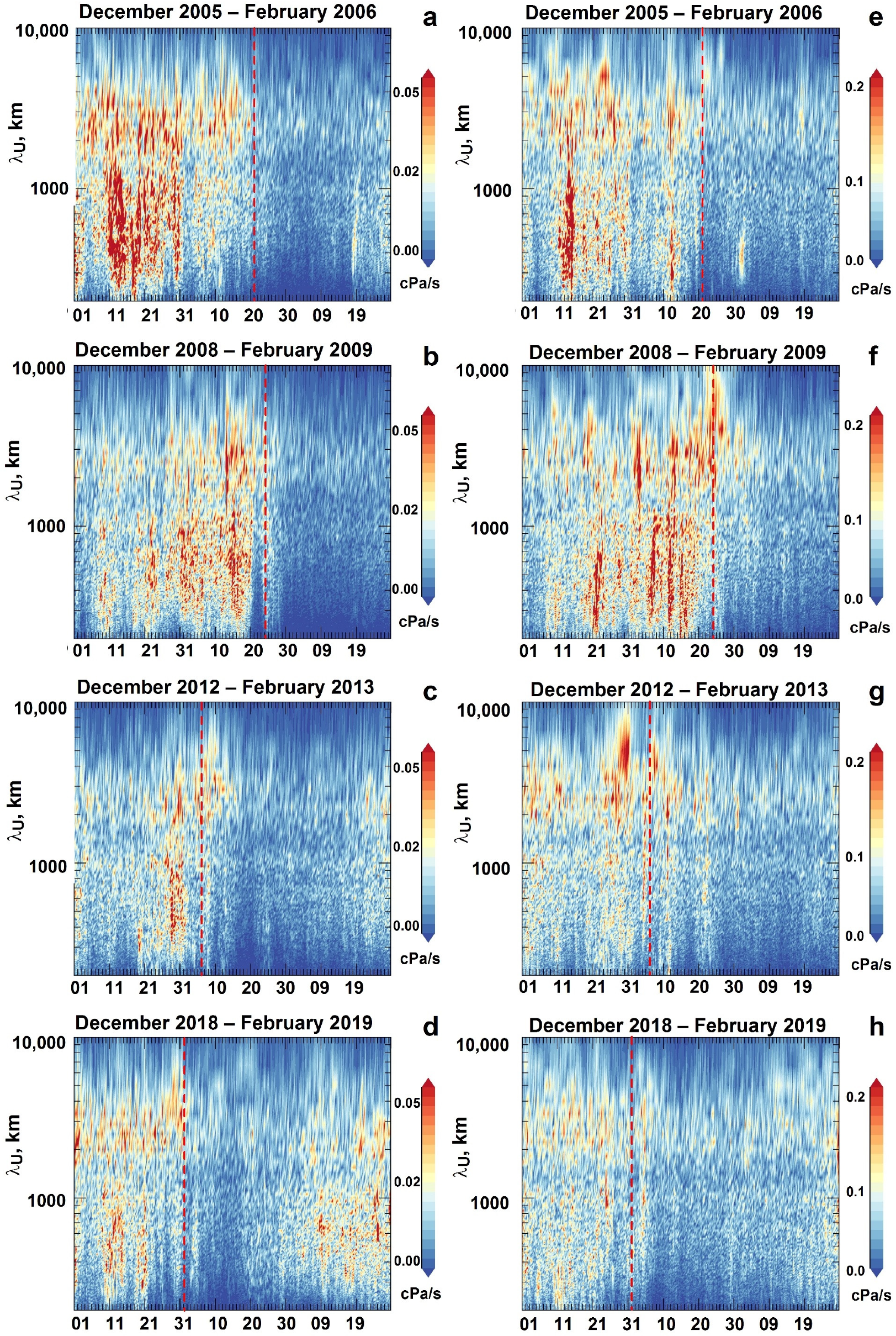
3.1. IGW Dynamics at Different SSW Stages

The paper addresses several north winter periods, during which strong major mid-winter stratospheric warmings occurred: 2005–2006, 2008–2009, 2012–2013, and 2018–2019. Figure 2 shows the distributions for the zonal mean of the zonal wind velocity at 60° N, depending on the height during the investigated winters. A major SSW features a change in the circulation direction in the stratosphere from west to east at 10 hPa (~30 km) and below in the middle to high latitudes. The day when the mid-zonal circulation reversal at the 10 hPa level was observed is referred to as the central date. The central dates for the above SSWs were recorded on 21 January 2006, 24 January 2009, 6 January 2013, and 1 January 2019, respectively. The periods selected for our analysis allowed us to trace the disturbance characteristic variations occurring during the SSW-related circulation restructuring in the stratosphere. Apparently, during the analyzed winters, the normal stratospheric circulation with the steady zonal flow was interrupted for over a month and even more.

Figure 3 and Figure 4 show, as examples, the distributions of the horizontal wind fields ν (a–e), the vertical velocity residual dW (f–j), and the zonal spectra of disturbances (k–o), depending on the latitude and the wavelength at the stratopause (1 hPa, Figure 3) and in the mid-stratosphere (10 hPa, Figure 4) on different days over December 2012–January 2013. The dates for the figures were selected to show different periods when the strong 2012/2013 SSW evolved. This period featured one of the strongest and most prolonged major SSWs, although it was weaker than the January 2009 record-breaking one. The central date for the 2012–2013 SSW was recorded on 6 January 2013, the temperature peak at 10 hPa was recorded at the same time.

Over an undisturbed winter period without a SSW, there is a well-defined JS on the horizontal wind distributions (Figure 3a and Figure 4a). The JS wind velocities may reach 150 m/s and more. The JS has a sufficiently symmetric ring structure. Moreover, one could observe distinct medium-scale wave disturbances in the vertical velocity residual distributions. The greatest intensities of the wave disturbances are recorded in the regions featuring the highest velocities of the JS horizontal wind (Figure 3f and Figure 4f).

During the SSW prewarming stage (at the end of December 2012), there was an essential JS transformation and its center displacement from the pole. The prewarming stage features an increase in the amplitude of planetary waves (with zonal harmonics 1 and/or 2), and enhancements in the wind shears [13]. This may lead to an increase in velocity of the JS (Figure 3b and Figure 4b). Consequently, the stratospheric jet stream structure changes dramatically. The duration of the stage can be about 2 weeks.

As the warming evolved in early January 2013, the CPV split into three vortices: two cyclonic vortices over Canada and western and central parts of the Eurasian continent; and an anticyclonic vortex over Siberia and the far east within the Eurasian continent (Figure 3c and Figure 4c), the region with the most efficient wave generation shifts following the JS displacement (Figure 3h and Figure 4h).

In the example of the addressed 2012–2013 winter SSW, wave disturbances were clearly visible, especially in the mid-stratosphere at the 10 hPa height (Figure 4f,g) on the days when there was a steady CPV (18 December 2012) and on the first days of the vortex transformations (26 December 2012). At the stage of CPV (and JS) weakening and the subsequent destruction (18 January 2013), there was a significant reduction in the generation of these small-scale wave disturbances; the amplitudes of these waves decreased (Figure 3i and Figure 4i). The area of spatial localization of wave disturbances was significantly reduced and shifted to middle latitudes. A similar scenario was observed at the 1 hPa height (stratopause—lower mesosphere) (Figure 3f-j).

The right panels (Figure 3 and Figure 4) show the spatial spectra of the vertical velocity residual depending on latitude. As one can see from the spectral distributions, the JS position determines the latitudinal variations in the disturbance intensity. In the quiet stratosphere, the spectra show the existence of a stable region for disturbance generation at 40–60° N, within the JS. One could observe variations with a broad spectrum—almost uniform by wavelengths at the stratopause level (1 hPa) and in the mid-stratosphere (10 hPa). At the stratopause level, in the mid-latitude region, disturbances with 500–1000 km wavelengths mainly occurred (18 December 2012) (Figure 3k). In the mid-stratosphere, wave disturbances with wavelengths up to 700 km were recorded in the mid-latitude region (Figure 4k). Such disturbance horizontal wavelengths in the atmosphere are characteristic of medium-scale IGWs. Similar spectral density distributions are constantly observed in the quiet winter stratosphere starting from the November second ten-day period for all the analyzed years. Analogous distributions were also obtained for periods of strong SSWs during the winters of 2005–2006, 2008–2009, and 2018–2019.

At the prewarming stage, on 26 December 2012, an increase in the wave variation intensity was observed (Figure 3l and Figure 4l). Moreover, we can note the emergence of disturbances of a larger horizontal wavelength, up to 3000–5000 km, mainly at high latitudes. The latitude range, in which the generation of disturbances occurred, extended to the high-latitude region (70–80° N).

After the major SSW maximum, there was a disruption of the polar vortex and the related JS; in this case, the wave disturbance generation stopped (on 8 and 18 January, Figure 3m,n and Figure 4m,n). At the mid-stratosphere altitude, the disturbance generation ceased earlier, but recovered later, compared to the stratopause level. On 4 February, at 1 hPa, one could observe a stratospheric vortex recovery and, accordingly, the generation of disturbances with 300–500 km wavelengths (Figure 3o). At the same time, the stratospheric vortex was not observed yet; moreover, there were almost no wave disturbances at the level of the mid-stratosphere (10 hPa) within this period (Figure 4o).

Figure 5 demonstrates the dynamic spectra of disturbances at 60° N, depending on the zonal wavelength at the stratopause–lower mesosphere level (1 hPa, left) and in the mid-stratosphere (10 hPa, right) during the 2005–2006, 2008–2009, 2012–2013, and 2018–2019 winters. The SSW central dates are marked on the panels by the vertical dotted lines.

For all the addressed winters, one could observe similar characteristic dynamics of disturbances. During quiet periods without SSW, a generation of wave disturbances occurred with the maxima in the spectrum falling into the zonal wavelengths of up to 1000 km prior to SSWs. Within a prewarming period, one could observe an increase in disturbances, as well as the emergence of larger-scale waves. The increase was most expressed at the mid-stratosphere level. After warming reached its maximum, and the JS was disrupted, one could observe a cessation of the disturbances of all the wavelengths. The stratospheric conditions remained undisturbed for a month and more after a SSW.

Thus, the results show that the generation of wave disturbances in the winter stratosphere was closely related to the winter JS dynamics and spatial position. The transformation and disruption of the CPV and the related JS, occurring during SSWs, led to a significant decrease (or even full cessation) of the generation of IGW in the stratosphere.

3.2. Estimates of Basic Parameters of the Observed Waves

An analytical description of the waves observed can be performed using the well-known Hines dispersion relation [40]:

$$k_h^2+k_z^2=\frac{k_h^2{\Omega }_B^2}{{\omega }^2}+\frac{{\omega }^2-{\omega }_A^2}{C_0^2},$$

(3)

here, Ω_B is the Brunt–Väisälä frequency, which is, according to theoretical estimates, ~0.02 s⁻¹, at the heights of the middle atmosphere [41]; k_z, k_h are the vertical and horizontal components of the wave vector; ${\omega }_A=\sqrt{g\gamma /4H}$ is the acoustic cutoff frequency; γ is the adiabatic index (so-called Poisson’s ratio), equal to the ratio of the thermal capacity at constant pressure C_P to the thermal capacity at constant volume C_V; H is the height of the homogeneous atmosphere; C₀—speed of sound. The second term of Equation (3) describes acoustic waves corresponding to high-frequency rolls (“vortex sheet”), which can propagate only near the active zone of the jet stream. The first term in Equation (3) corresponds to internal gravity waves, the frequencies of which are determined by the expression:

$${\omega }^2=\frac{{\Omega }_B^2}{1+k_z^2/k_h^2}=\frac{{\Omega }_B^2}{1+{\lambda }_h^2/{\lambda }_z^2}\cong {\Omega }_B^2{\lambda }_z^2/{\lambda }_h^2={\Omega }_B^2{\cos }^2\theta ,$$

(4)

here, θ is the propagation angle; λ_z, λ_h—vertical and horizontal wavelengths. As noted above, in the quiet stratosphere, the zonal wavelength λ_U almost completely coincides with the horizontal one and λ_h can be determined from the spectra of vertical velocity variations. Thus, the horizontal wavelength varies over a wide range λ_h = 300–1000 km.

Distributions of vertical velocity variations in height from ERA-5 data make it possible to estimate that the vertical wavelength λ_z ~ 10 km. Thus, taking into account these parameters, it can be roughly estimated that typical periods of wave disturbances observed at heights of the strato–mesosphere can be T = 50–150 min, i.e., periods of medium-scale IGWs.

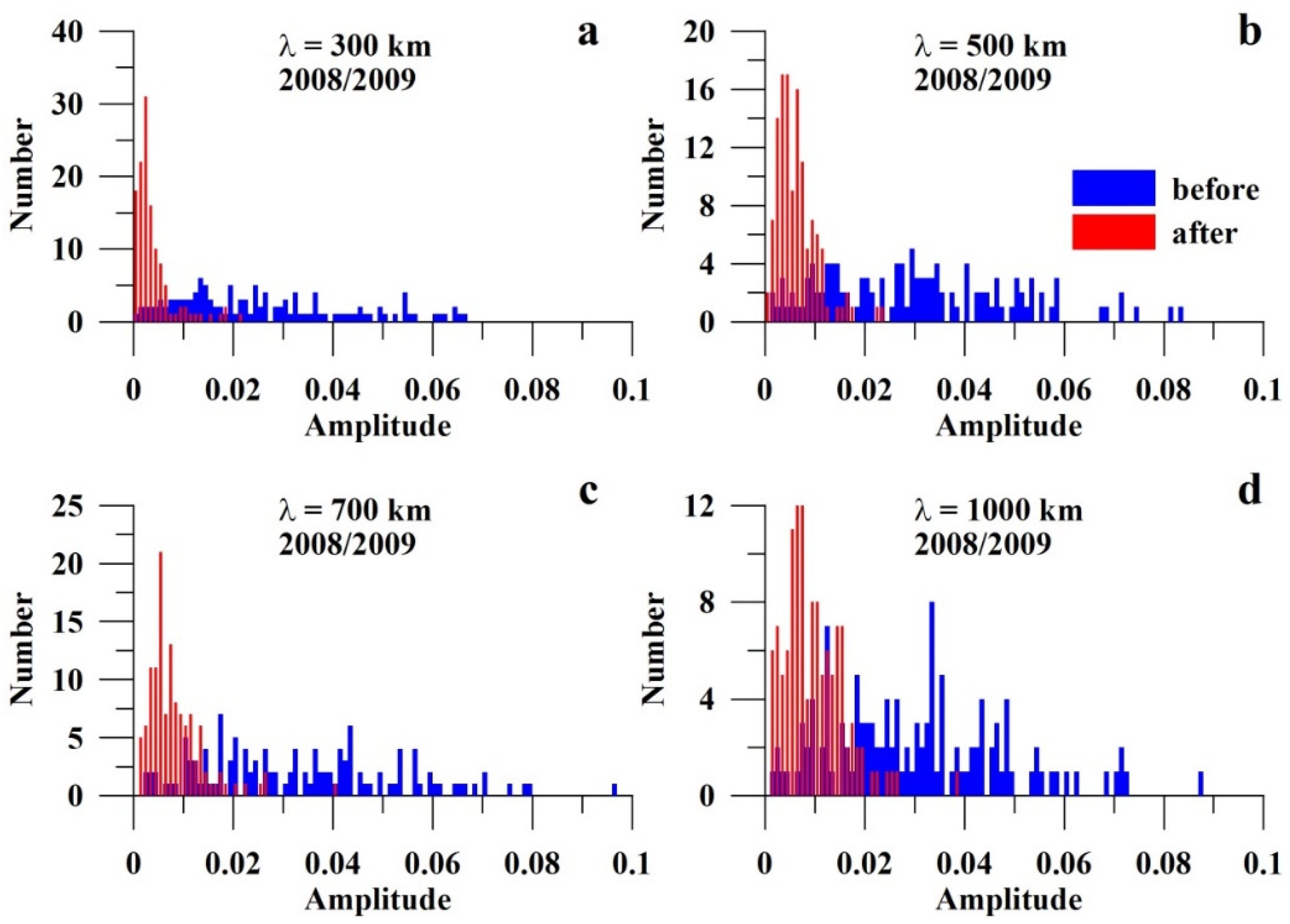
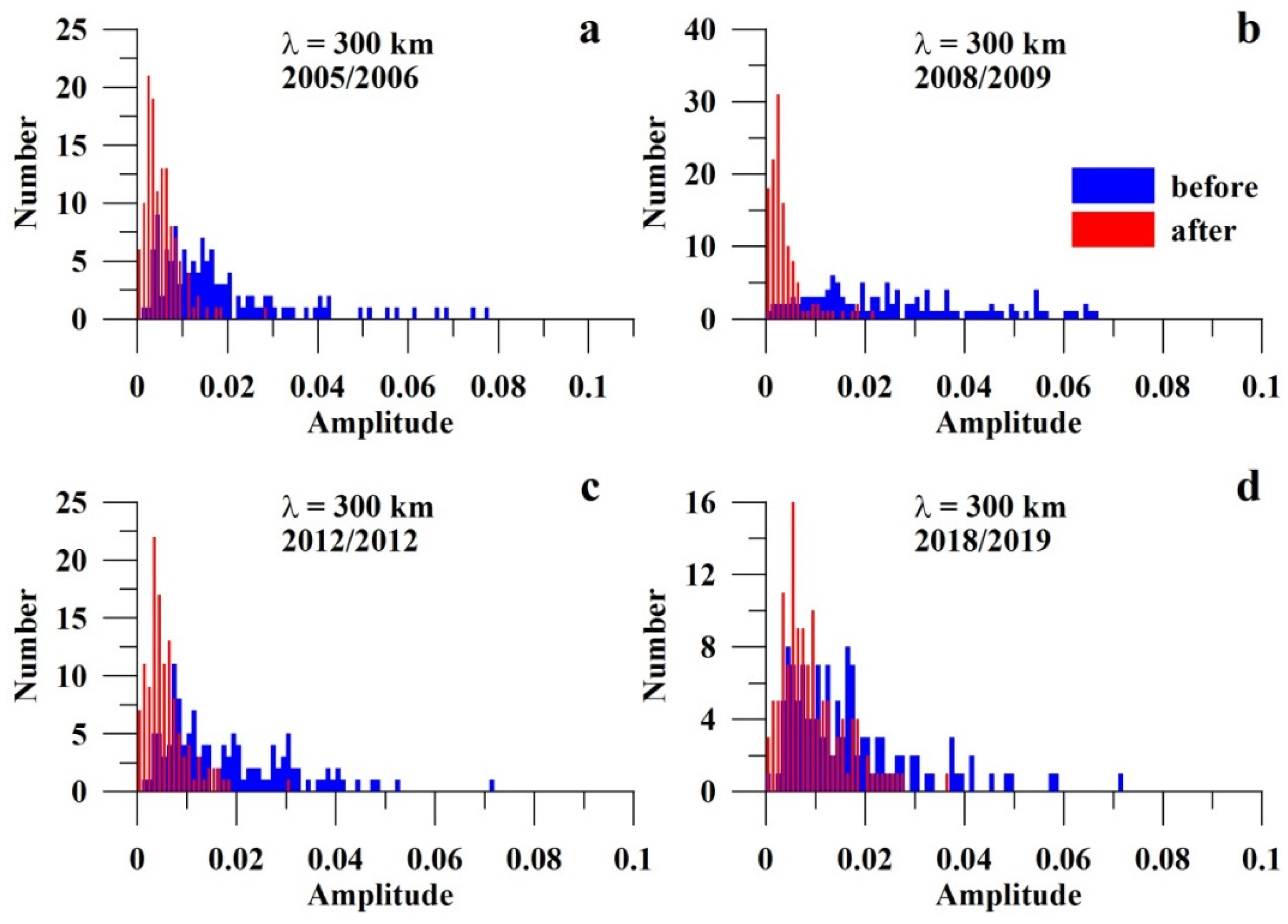
3.3. Statistical Estimates of the Observed Effect

To assess the significance of the observed effect, we performed a statistical significance test for the amplitude distributions shown in Figure 5. For this purpose, the amplitudes for a set of different zonal wavelengths (λ_U = 300, 500, 700, 1000 km) were addressed. The amplitude values at each wavelength were sorted into two samples: 30 days before and 30 days after the peak date of the corresponding SSW event. Then, we built amplitude distributions for each sample and evaluated the Student’s significance test. The statistical significance criteria p-values represent the probability that the addressed subsamples belong to the same distribution. We also estimated the ratio of the amplitude mean values before the SSW peak date to the value of the amplitudes after the latter.

Figure 6 provides the examples of the amplitude distributions for zonal wavelengths of 300 (a), 500 (b), 700 (c), and 1000 (d) km before (blue) and after the (red) SSW peak dates during the 2008/2009 winter at the 1 hPa level. Figure 7 provides similar distributions, but for the 300 km wavelength in the 2005/2006 (a), 2008/2009 (b), 2012/2013 (c), and 2018/2019 (d) winters at the 1 hPa level.

Table 1. Ratio of the average amplitude before and after the peak dates of the SSWs for different zonal wavelengths at the 1 hPa level. The significance criteria p-values are given in brackets.

λU, km	2005/2006	2008/2009	2012/2013	2018/2019
300	3.25 (p = 7.2 × 10−16)	6.73 (p = 6.9 × 10−26)	3.05 (p = 3.7 × 10−19)	1.81 (p = 9.9 × 10−9)
500	2.57 (p = 5.7 × 10−15)	2.81 (p = 1.8 × 10−28)	2.34 (p = 1.4 × 10−15)	1.75 (p = 1.0 × 10−9)
700	2.37 (p = 8.6 × 10−18)	3.98 (p = 4.5 × 10−28)	1.86 (p = 5.8 × 10−11)	1.82 (p = 5.8 × 10−14)
1000	2.53 (p = 8.8 × 10−18)	3.16 (p = 1.0 × 10−22)	1.85 (p = 2.1 × 10−13)	1.86 (p = 4.4 × 10−14)

presents the values of the obtained ratios and p-value criteria for amplitude distributions at the 1 hPa level.

One can see from Figure 6 and Figure 7 and values in Table 1 that, for all the addressed cases, there is a statistically significant shift of the distribution to the domain of lower amplitude values (statistical significance p-value < 10⁻⁸—i.e., the probability that subsamples before and after the SSW peak belong to the same distribution is small and this null hypothesis can be discarded).

After the SSW peak dates, decreases in the average amplitude values (by factors of 1.8–6.7) were recorded. The strongest amplitude drop was observed for short waves λ_U = 300 km. The most powerful effect on amplitude change was recorded for the 2008–2009 SSW, which was the strongest one. The weakest effect was observed in 2018–2019; that SSW event featured the smallest power and duration.

4. Discussion

For all of the addressed SSW events, there was a significant and statistically relevant decrease in the amplitude of waves generated in the JS. A decrease in the intensity of small-scale wave disturbance after the peaks for all of the addressed SSWs confirms that it is the JS itself that is a source for IGW generation at the strato–mesosphere through the mechanism proposed in [35]. The mechanism suggests that wave disturbances with IGW periodicity appear directly inside the polar vortex and that wave generation is not associated with an increase in the activity of planetary waves, propagating upward from the troposphere into the stratosphere and disturbing the prevailing zonal flow. According to Shpynev et al. [35], the structure of the mid-latitude and polar strato–mesosphere in winter is a complex spiral circulation, consisting of a system of flat, almost horizontal jet streams located at 40–60° latitudes. The most interesting phenomenon in the structure is the presence of a spiral boundary layer between the streams. Inside the vortex, conditions for the formation of baroclinic-type instabilities appear, which generate atmospheric waves of various scales.

During SSWs, powerful downward flows with vertical velocities of more than 1 m/s emerge in the stratosphere. Owing to this, strong periodic inhomogeneities are generated within a large altitude range (~15–45 km). When the JS vertical velocity exceeds some critical value (~1 m/s at 10 hPa) and the Reynolds number is high, the wave amplitude increases to very high values. Waves may overturn, transferring to an extreme case of Kelvin–Helmholtz waves. These strong wave disturbances are similar, for clarity of understanding, to rolls observed in tropospheric thunderstorm clouds. Roll clouds usually appear to be “rolling” about a horizontal axis; they are completely detached from the convective storm cloud base. So, these stratospheric wave structures (emerging as a result of IGW breaking) convert the impinging stream potential energy to the stratosphere heating and contribute significantly to the effect of the temperature increase during SSWs. These waves are sometimes referred to as a “vortex sheet” in fluid mechanics terminology for a surface across which there is a discontinuity in the fluid velocities, such as in the slippage of one layer of fluid over another. The spatial scale of rolls is the IGW limiting minimal scale that varies with height, i.e., it depends on the Brunt–Väisälä frequency.

Apparently, when the JS velocity is higher (as during SSW prewarming stage), more energy of the instabilities can be spent to generate IGWs, including larger-scale IGWs. On the contrary, when the wind speed in the JS falls below certain threshold values (as after SSW peak), the conditions for the occurrence of baroclinic instability and, as a consequence wave generation, disappear.

The stratospheric wave disturbances composing the high-frequency part of the spectrum will be conversed, primarily, to warm, due to a cascade destruction of atmospheric vortices and turbulent diffusion [35,39]. The medium-scale IGWs (1000–3000 km) emerging at the altitudes higher ~40 km propagate mainly toward the mesosphere, where they are reflected or absorbed at 85–100 km high. Part of those IGWs may penetrate the thermosphere. Thus, the stratopause region is a natural barrier, below which the energy of JS instabilities is converted into stratosphere heating. The IGWs generated above the stratopause are steadier to turbulent damping and may propagate at various angles upward for large distances [42]. Simultaneously, such IGWs implement dynamic coupling between different atmospheric layers.

Comparing the wave disturbances in the parameters of the neutral atmosphere and the ionosphere may provide information on the processes stipulating the dynamic coupling between various atmospheric layers [43]. Thus, the emergence of an IGW stratospheric source during the winter period and its deactivation after strong SSW maxima may be reflected in the upper-atmosphere disturbance dynamics.

The relation between variations in the stratosphere and higher layers of the atmosphere was studied in previous works. For example, Medvedeva and Ratovsky [44], based on the hydroxyl emission spectral observations, concluded that the seasonal variations in the mesosphere variabilities have well-pronounced maximums in the winter months. Frissell et al. [27] and Yasyukevich et al. [45] showed that there is an essential correlation between the disturbance in the ionosphere and the CPV dynamics. Yigit and Medvedev [46] noted a possible role of gravity waves in vertical coupling between the lower and the upper atmospheres during SSW events.

The authors [47,48] noted a possible relation between the increase in the winter ionospheric disturbance and the JS dynamics over the Eurasian region during the 2008/2009 and 2012/2013 SSW events. The authors revealed that ionospheric disturbances significantly depend on the ionosonde position relative to the JS location. They suggested two general mechanisms for the underlying atmosphere’s impact on the ionosphere. The first assumed mechanism was the molecular gas upwelling/downwelling to/from the lower thermosphere. Another proposed mechanism was the transport of the molecular species due to activity of IGWs, which disturbed the boundary between the molecular and the atomic atmosphere.

Lukianova et al. [49], based on meteor radar measurements, recorded the decay of gravity waves with 10–60 min periods in the ionosphere over Sodankyla during the 2009 SSW. However, the interpretation of that result remained vague.

Nayak and Yigit [50] studied the 2009 major SSW event effect on the small-scale IGW activity in the ionosphere. They showed that, at the warming initial phase, the IGW activity tended to increase. However, during and after the SSW peak, the IGW activity was reduced. The author suggested that, during the latter period of the SSW, conditions were less favorable for upward propagation of a spectrum of IGWs and, thus, the ionospheric disturbances were weaker. A similar reduction in the IGW activity was also observed in the middle atmosphere (65–100 km).

The results of our study suggest that the main reason for the decrease in the IGW activity observed in the upper atmospheric layers during SSW in previous studies [49,50] could be the cessation of wave generation in the strato–mesosphere due to the JS weakening/disruption.

5. Conclusions

We analyzed the parameters of small-scale wave disturbances emerging during the evolution of the winter CPV, with special attention to periods of major SSW events. In undisturbed winter periods, when a stable JS forms in the stratosphere, a constant generation of wave disturbances with a broad spectrum of horizontal wavelengths was shown to occur. The horizontal lengths of most intensive disturbances varied from 300 to 1000 km and periods within 50–150 min. The estimates of typical scales for the observed disturbances corresponded to internal gravity waves. The greatest intensity disturbances were recorded in regions that corresponded to high JS velocities (from 100 m/s and higher). In the northern hemisphere, this implied ~40–60° N.

At the SSW prewarming stage, the JS changed substantially. In the spatial variation spectra, one recorded an intensification of disturbances and the emergence of large-scale disturbances at high latitudes (70–80° N) with horizontal wavelengths up to 3000–5000 km. There was also an expansion of the latitudinal range, in which disturbances were generated to the regions of high latitudes that were due to the JS shift.

After major SSWs, there was an essential attenuation (and even cessation) in the generation of wave disturbances. There were decreases in the average amplitude values (by factors of 1.8–6.7). The strongest amplitude drop was observed for short waves λ_U = 300 km. The maximum attenuation for all wavelengths was observed for the strongest 2008/2009 winter SSWs. Such attenuation was related to the JS disruption and was observed for about one month after the SSW maximum. Thus, major SSW events lead to deactivating the disturbance source in the strato–mesosphere for a long-term time interval.

Significant decreases in the intensities of small-scale wave disturbances after the peaks for all of the addressed SSWs confirmed the mechanism for IGW generation in the JS proposed in [35]. The results of our study are particularly relevant for studying the coupling between different atmosphere layers during SSW events and provide valuable information for further investigations of the correlation between disturbances at different atmospheric layers. We provide evidence that the main reason for the decrease in the IGW activity in the upper atmospheric layers during SSWs observed in previous studies could be the cessation of wave generation in the strato–mesosphere due to the JS weakening/disruption.

Further detailed studies may include using modern optical systems [51], as well as revealing the relation with disturbances in the upper atmosphere [52].

References

1. Coy, L.; Nash, E.R.; Newman, P.A. Meteorology of the polar vortex: Spring 1997. Geophys. Res. Lett. 1997, 24, 2693–2696. [Google Scholar] [CrossRef]
2. Newman, P.A.; Schoeberl, M.R. Middle atmosphere: Polar vortex. In Encyclopedia of Atmospheric Sciences; Holton, J.R., Pyle, J., Curry, J.A., Eds.; Academic Press: San Diego, CA, USA, 2003; pp. 1321–1328. [Google Scholar]
3. Waugh, D.W.; Polvani, L.M. Stratospheric polar vortices. In The Stratosphere: Dynamics, Transport, and Chemistry; Polvani, L.M., Sobel, A.H., Waugh, D.W., Eds.; Geophysical Monograph Series; American Geophysical Union: Washington, DC, USA, 2010; Volume 190, pp. 43–57. [Google Scholar] [CrossRef]
4. Schoeberl, M.R.; Hartmann, D.L. The dynamics of the stratospheric polar vortex and its relation to springtime ozone depletions. Science 1991, 251, 46–52. [Google Scholar] [CrossRef]
5. Karpetchko, A.; Kyrö, E.; Knudsen, B.M. Arctic and Antarctic polar vortices 1957–2002 as seen from the ERA-40 reanalyses. J. Geophys. Res. 2005, 110, D21109. [Google Scholar] [CrossRef]
6. Hamilton, K. Dynamical coupling of the lower and middle atmosphere: Historical background to current research. J. Atmos. Sol.-Terr. Phys. 1999, 61, 73–84. [Google Scholar] [CrossRef]
7. Labitzke, K.G.; van Loon, H. The Stratosphere: Phenomena, History, and Relevance; Springer: New York, NY, USA, 1999; 179p. [Google Scholar]
8. Sun, L.; Robinson, W.A. Downward influence of stratospheric final warming events in an idealized model. Geophys. Res. Lett. 2009, 36, L03819. [Google Scholar] [CrossRef]
9. Baldwin, M.P.; Dunkerton, T.J. Stratospheric harbingers of anomalous weather regimes. Science 2001, 294, 581–584. [Google Scholar] [CrossRef]
10. Kushner, P.J. Annular modes of the troposphere and stratosphere. In The Stratosphere: Dynamics, Transport, and Chemistry; Polvani, L.M., Sobel, A.H., Waugh, D.W., Eds.; Geophysical Monograph Series; American Geophysical Union: Washington, DC, USA, 2010; Volume 190, pp. 59–91. [Google Scholar] [CrossRef]
11. Pogoreltsev, A.I.; Aniskina, O.G.; Ermakova, T.S.; Savenkova, E.N.; Chen, W.; Wei, K. Interannual and intraseasonal variability of stratospheric dynamics and stratosphere-troposphere coupling during northern winter. J. Atmos. Sol.-Terr. Phys. 2015, 136, 187–200. [Google Scholar] [CrossRef]
12. Waugh, D.W.; Sobel, A.H.; Polvani, L.M. What is the polar vortex and how does it influence weather? Bull. Am. Meteorol. Soc. 2017, 98, 37–44. [Google Scholar] [CrossRef]
13. Schoeberl, M.R. Stratospheric warmings: Observations and theory. J. Geophys. Res. Space Phys. 1978, 16, 521–538. [Google Scholar] [CrossRef]
14. Baldwin, M.P.; Holton, J.R. Climatology of the stratospheric polar vortex and planetary wave breaking. J. Atmos. Sci. 1988, 45, 1123–1142. [Google Scholar] [CrossRef]
15. Abatzoglou, J.T.; Magnusdottir, G. Wave breaking along the stratospheric polar vortex as seen in ERA-40 data. Geophys. Res. Lett. 2007, 34, L08812. [Google Scholar] [CrossRef]
16. Kim, B.M.; Son, S.W.; Min, S.K.; Jeong, J.H.; Kim, S.J.; Zhang, X.; Shim, T.; Yoon, J.H. Weakening of the stratospheric polar vortex by Arctic sea-ice loss. Nat. Commun. 2014, 5, 4646. [Google Scholar] [CrossRef]
17. Zhang, J.; Tian, W.; Chipperfield, M.P.; Xie, F.; Huang, J. Persistent shift of the Arctic polar vortex towards the Eurasian continent in recent decades. Nat. Clim. Chang. 2016, 6, 1094–1099. [Google Scholar] [CrossRef]
18. Seviour, W.J. Weakening and shift of the Arctic stratospheric polar vortex: Internal variability or forced response? Geophys. Res. Lett. 2017, 44, 3365–3373. [Google Scholar] [CrossRef]
19. Labitzke, K. Temperature changes in the mesosphere and stratosphere connected with circulation changes in winter. J. Atmos. Sci. 1972, 29, 756–766. [Google Scholar] [CrossRef]
20. Stan, C.; Straus, D.M. Stratospheric predictability and sudden stratospheric warming events. J. Geophys. Res. Atmos. 2009, 114, D12103. [Google Scholar] [CrossRef]
21. Matsuno, T. A dynamical model of the stratospheric sudden warming. J. Atmos. Sci. 1971, 28, 1479–1494. [Google Scholar] [CrossRef]
22. Scott, R.K.; Polvani, L.M. Internal Variability of the Winter Stratosphere. Part I: Time-Independent Forcing. J. Atmos. Sci. 2006, 63, 2758–2776. [Google Scholar] [CrossRef]
23. Pogoreltsev, A.I.; Vlasov, A.A.; Fröhlich, K.; Jacobi, C. Planetary waves in coupling the lower and upper atmosphere. J. Atmos. Sol.-Terr. Phys. 2007, 69, 2083–2101. [Google Scholar] [CrossRef]
24. Charlton, A.J.; Polvani, L.M. A new look at stratospheric sudden warmings. Part I: Climatology and modeling benchmarks. J. Clim. 2007, 20, 449–469. [Google Scholar] [CrossRef]
25. Whiteway, J.A.; Duck, T.J.; Donovan, D.P.; Bird, J.C.; Pal, S.R.; Carswell, A.I. Measurements of gravity wave activity within and around the Arctic stratospheric vortex. Geophys. Res. Lett. 1997, 24, 1387–1390. [Google Scholar] [CrossRef]
26. Gerrard, A.J.; Bhattacharya, Y.; Thayer, J.P. Observations of in-situ generated gravity waves during a stratospheric temperature enhancement (STE) event. Atmos. Chem. Phys. 2011, 11, 11913–11917. [Google Scholar] [CrossRef]
27. Frissell, N.A.; Baker, J.B.H.; Ruohoniemi, J.M.; Greenwald, R.A.; Gerrard, A.J.; Miller, E.S.; West, M.L. Sources and characteristics of medium-scale traveling ionospheric disturbances observed by high-frequency radars in the North American sector. J. Geophys. Res. Space Phys. 2016, 121, 3722–3739. [Google Scholar] [CrossRef]
28. Liu, X.; Yue, J.; Xu, J.; Garcia, R.R.; Russell, J.M., III; Mlynczak, M.; Wu, D.L.; Nakamura, T. Variations of global gravity waves derived from 14 years of SABER temperature observations. J. Geophys. Res. Atmos. 2017, 122, 6231–6249. [Google Scholar] [CrossRef]
29. Wu, D.L.; Waters, J.W. Satellite observations of atmospheric variances: A possible indication of gravity waves. Geophys. Res. Lett. 1996, 23, 3631–3634. [Google Scholar] [CrossRef]
30. Jiang, J.H.; Eckermann, S.D.; Wu, D.L.; Hocke, K.; Wang, B.; Ma, J.; Zhang, Y. Seasonal variation of gravity wave sources from satellite observation. Adv. Space Res. 2005, 35, 1925–1932. [Google Scholar] [CrossRef]
31. Jiang, J.H.; Wu, D.L.; Wang, D.-Y. Interannual variation of gravity waves in the Arctic and Antarctic winter middle atmosphere. Adv. Space Res. 2006, 38, 2418–2423. [Google Scholar] [CrossRef]
32. Wilson, R.; Chanin, M.-L.; Hauchecorne, A. Gravity waves in the middle atmosphere observed by Rayleigh lidar. Part 2. Climatology. J. Geophys. Res. 1991, 96, 5169–5183. [Google Scholar] [CrossRef]
33. Yamashita, C.; Liu, H.-L.; Chu, X. Gravity wave variations during the 2009 stratospheric sudden warming as revealed by ECMWF-T799 and observations. Geophys. Res. Lett. 2010, 37, L22806. [Google Scholar] [CrossRef]
34. Schoon, L.; Zülicke, C. A novel method for the extraction of local gravity wave parameters from gridded three-dimensional data: Description, validation, and application. Atmos. Chem. Phys. 2018, 18, 6971–6983. [Google Scholar] [CrossRef]
35. Shpynev, B.G.; Churilov, S.M.; Chernigovskaya, M.A. Generation of waves by jet-stream instabilities in winter polar stratosphere/mesosphere. J. Atmos. Sol.-Terr. Phys. 2015, 136, 201–215. [Google Scholar] [CrossRef]
36. Shpynev, B.G.; Khabituev, D.S.; Chernigovskaya, M.A.; Zorkal’tseva, O.S. Role of winter jet stream in the middle atmosphere energy balance. J. Atmos. Sol.-Terr. Phys. 2019, 188, 1–10. [Google Scholar] [CrossRef]
37. Vadas, S.L. Horizontal and vertical propagation of gravity waves in thermosphere from lower atmospheric and thermospheric sources. J. Geophys. Res. 2007, 112, A06305. [Google Scholar] [CrossRef]
38. Hersbach, H.; Bell, B.; Berrisford, P.; Hirahara, S.; Horányi, A.; Muñoz-Sabater, J.; Nicolas, J.; Peubey, C.; Radu, R.; Schepers, D.; et al. The ERA5 global reanalysis. QJR Meteorol Soc. 2020, 146, 1999–2049. [Google Scholar] [CrossRef]
39. Shpynev, B.G.; Chernigovskaya, M.A.; Khabituev, D.S. Spectral characteristics of atmospheric waves generated by winter stratospheric jet stream in the Northern Hemisphere. Sovrem. Probl. Distantsionnogo Zondirovaniya Zemli Kosm. 2016, 13, 120–131. [Google Scholar] [CrossRef]
40. Hines, C.O. Internal atmospheric gravity waves at ionospheric heights. Can. J. Phys. 1960, 38, 1441–1481. [Google Scholar] [CrossRef]
41. Gossard, E.E.; Hooke, W.H. Waves in the Atmosphere: Atmospheric Infrasound and Gravity Waves: Their Generation and Propagation, Developments in Atmospheric Science; Elsevier Scientific Pub. Co.: Amsterdam, The Netherlands; New York, NY, USA, 1975; Volume 2, 456p. [Google Scholar]
42. Kaifler, B.; Lübken, F.-J.; Höffner, J.; Morris, R.J.; Viehl, T.P. Lidar observations of gravity wave activity in the middle atmosphere over Davis (69°S, 78°E), Antarctica. J. Geophys. Res. Atmos. 2015, 120, 4506–4521. [Google Scholar] [CrossRef]
43. Liu, H.-L.; Yudin, V.A.; Roble, R.G. Day-to-day ionospheric variability due to lower atmosphere perturbations. Geophys. Res. Lett. 2013, 40, 665–670. [Google Scholar] [CrossRef]
44. Medvedeva, I.; Ratovsky, K. Studying atmospheric and ionospheric variabilities fromlong-termspectrometric and radio sounding measurements. J. Geophys. Res. Space Phys. 2015, 120, 5151–5159. [Google Scholar] [CrossRef]
45. Yasyukevich, A.; Medvedeva, I.; Sivtseva, V.; Chernigovskaya, M.; Ammosov, P.; Gavrilyeva, G. Strong Interrelation between the Short-Term Variability in the Ionosphere, Upper Mesosphere, and Winter Polar Stratosphere. Remote Sens. 2020, 12, 1588. [Google Scholar] [CrossRef]
46. Yiğit, E.; Medvedev, A.S. Internal waves coupling processes in Earth’s atmosphere. Adv. Space Res. 2015, 55, 983–1003. [Google Scholar] [CrossRef]
47. Chernigovskaya, M.A.; Shpynev, B.G.; Ratovsky, K.G. Meteorological effects of ionospheric disturbances from vertical radio sounding data. J. Atmos. Sol.-Terr. Phys. 2015, 136, 235–243. [Google Scholar] [CrossRef]
48. Chernigovskaya, M.A.; Shpynev, B.G.; Ratovsky, K.G.; Belinskaya, A.Y.; Stepanov, A.E.; Bychkov, V.V.; Grigorieva, S.A.; Panchenko, V.A.; Korenkova, N.A.; Mielich, J. Ionospheric Response to Winter Stratosphere/Lower Mesosphere Jet stream in the Northern Hemisphere as Derived from Vertical Radio Sounding Data. J. Atmos. Sol.-Terr. Phys. 2018, 180, 126–136. [Google Scholar] [CrossRef]
49. Lukianova, R.; Kozlovsky, A.; Shalimov, S.; Ulich, T.; Lester, M. Thermal and dynamical perturbations in the winter polar mesosphere-lower thermosphere region associated with sudden stratospheric warmings under conditions of low solar activity. J. Geophys. Res. Space Phys. 2015, 120, 5226–5240. [Google Scholar] [CrossRef]
50. Nayak, C.; Yigit, E. Variation of small-scale gravity wave activity in the ionosphere during the major sudden stratospheric warming event of 2009. J. Geophys. Res. Space Phys. 2019, 124, 470–488. [Google Scholar] [CrossRef]
51. Vasilyev, R.V.; Artamonov, M.F.; Beletsky, A.B.; Zorkaltseva, O.S.; Komarova, E.S.; Medvedeva, I.V.; Mikhalev, A.V.; Podlesny, S.V.; Ratovsky, K.G.; Syrenova, T.E.; et al. Scientific goals of optical instruments of the National Heliogeophysical Complex. Sol.-Terr. Phys. 2020, 6, 84–97. [Google Scholar] [CrossRef]
52. Yasyukevich, A.S. Features of short-period variability of total electron content at high and middle latitudes. Sol.-Terr. Phys. 2021, 7, 71–78. [Google Scholar] [CrossRef]
Figure 1. Example for the vertical velocity field W (top) and the residual dW (bottom) at the 1 hPa level on 25 December 2012 0 UT (polar view from the North Pole).
Remotesensing 14 02798 g001
Figure 2. Distributions for the zonal mean of zonal wind at 60° N, depending on the height, within the 2005–2006 (a), 2008–2009 (b), 2012–2013 (c), and 2018–2019 (d) winters.
Remotesensing 14 02798 g002
Figure 3. Distributions for the horizontal wind fields ν (ae), the vertical velocity residual dW (fj), and the spectral densities of the observed disturbances (ko), depending on the latitude and the zonal wavelength at the stratopause level (1 hPa) on different days of the 2012–2013 winter. Dates are on the left panels. The arrows on the left panels show the direction of the air mass travel. Distributions of velocities are presented in polar coordinates for the latitude interval 15°–90° N.
Remotesensing 14 02798 g003
Figure 4. Distributions for the horizontal wind fields ν (ae), the vertical velocity residual dW (fj), and the spectral densities of the observed disturbances (ko), depending on the latitude and the zonal wavelength in the mid-stratosphere (10 hPa) on different days of the 2012–2013 winter. Dates are on the left panels. The arrows on the left panels show the direction of the air mass travel. Distributions of velocities are presented in polar coordinates for the latitude interval 15°–90° N.
Remotesensing 14 02798 g004
Figure 5. Dynamic spectra of disturbances, depending on the zonal wavelength at the stratopause level (1 hPa, ad) and in the mid-stratosphere (10 hPa, eh) at 60° N during the 2005–2006, 2008–2009, 2012–2013, and 2018–2019 winters.
Remotesensing 14 02798 g005
Figure 6. Amplitude distributions for zonal wavelengths of 300 (a), 500 (b), 700 (c), and 1000 (d) km before (blue) and after (red) the SSW peak dates in the 2008/2009 winter at the 1 hPa level.
Remotesensing 14 02798 g006
Figure 7. Amplitude distributions for zonal wavelengths of 300 km before (blue) and after (red) the SSW peak dates in the 2005/2006 (a), 2008/2009 (b), 2012/2013 (c), and 2018/2019 (d) winter at the 1 hPa level.
Remotesensing 14 02798 g007