
Comparison of Machine Learning-Based Snow Depth Estimates and Development of a New Operational Retrieval Algorithm over China

 , , ,
, , ,  , and
, and
Abstract
:1. Introduction
2. Data and Methodology
2.1. Ground-Based Measurements
2.2. Gridded Products
2.3. ML Models
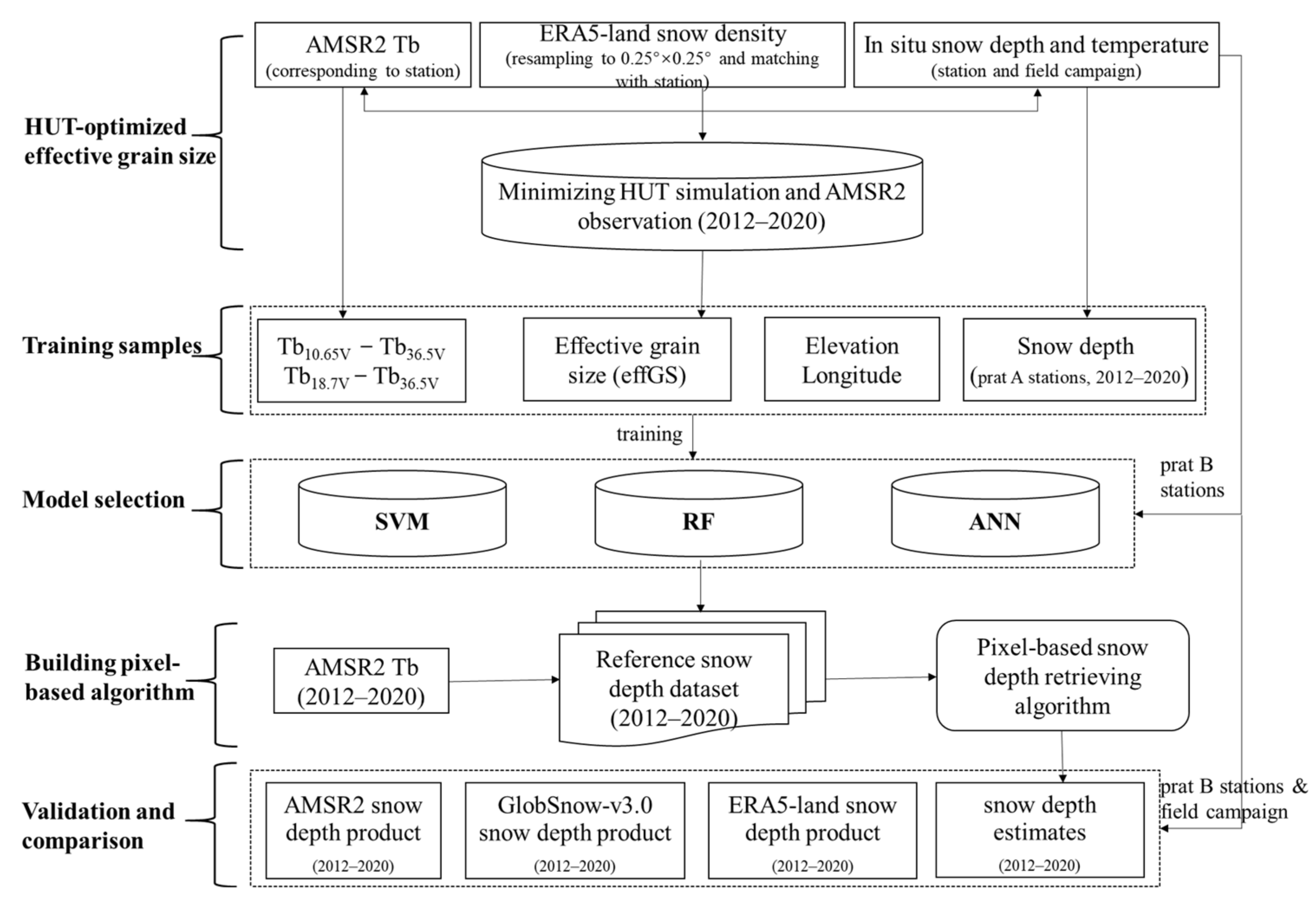
2.4. Workflow
3. Results
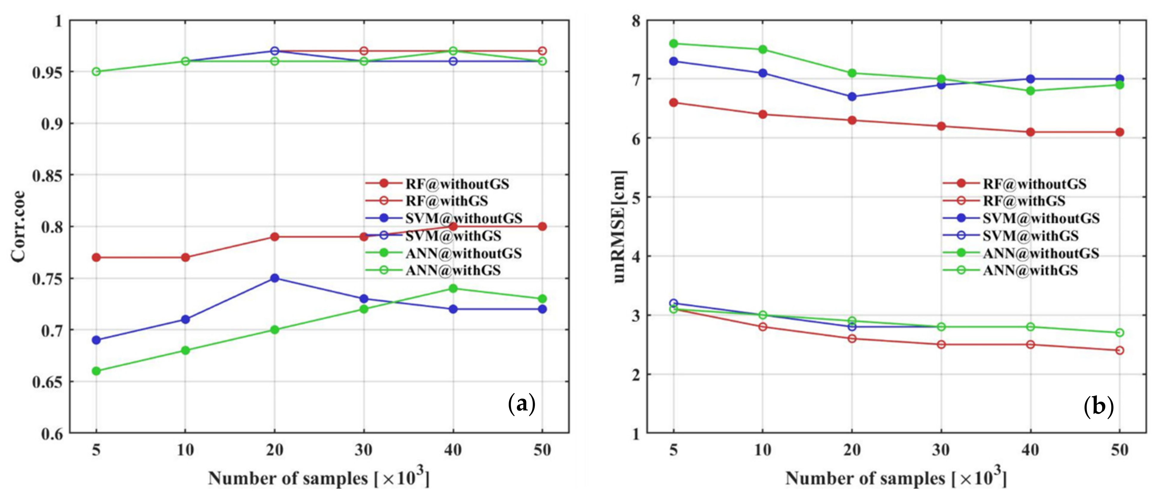
3.1. Sensitivity of ML Models to Training Sample Size
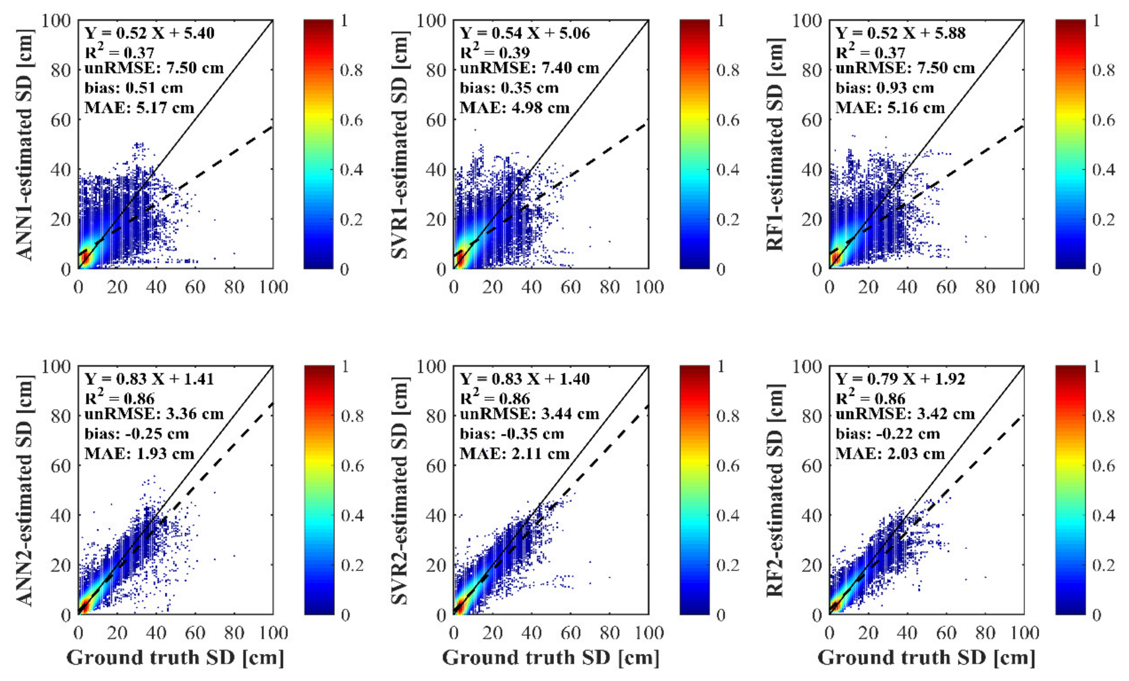
3.2. ML Model Performances
3.3. Development of the Pixel-Based Algorithm
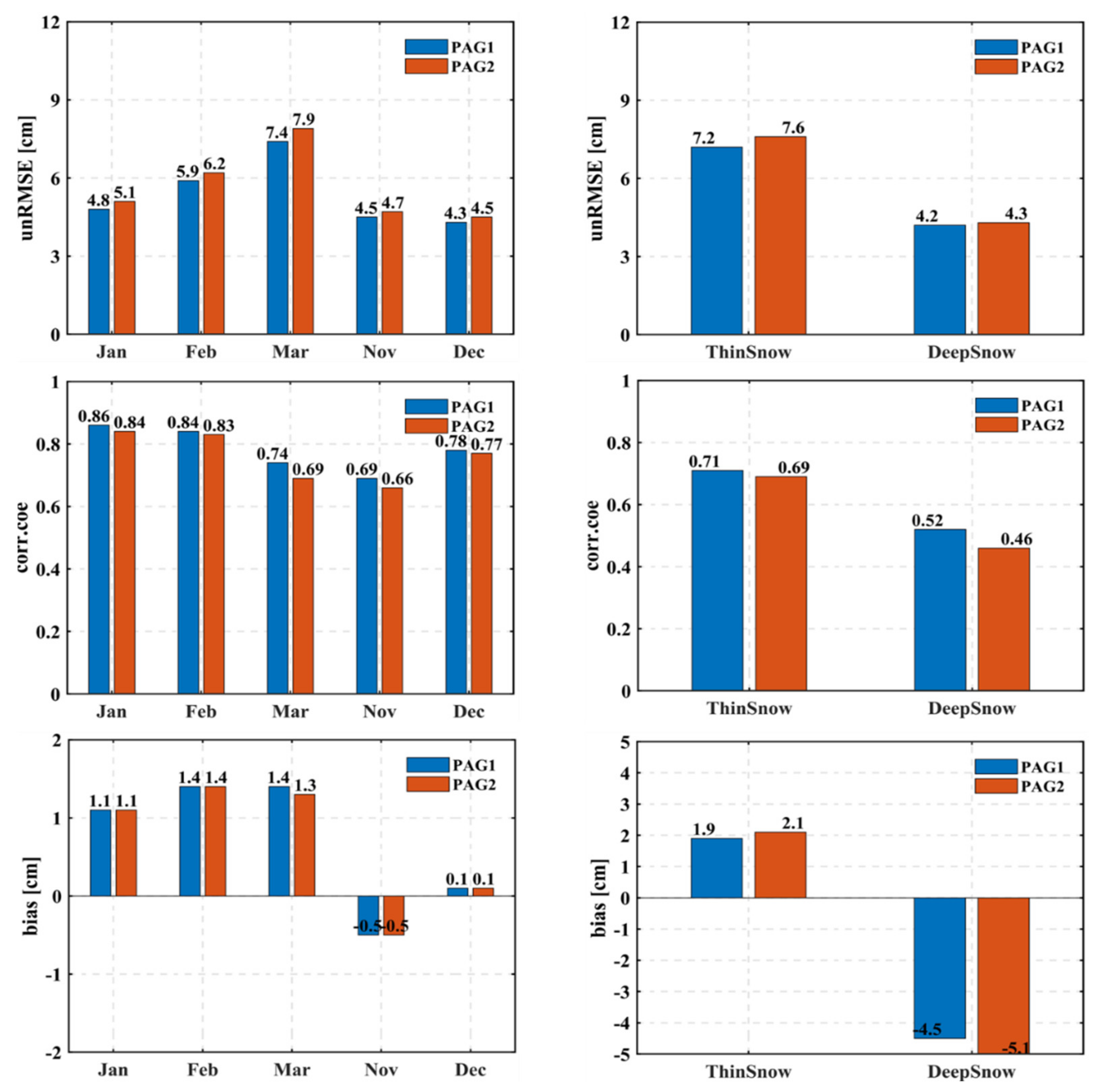
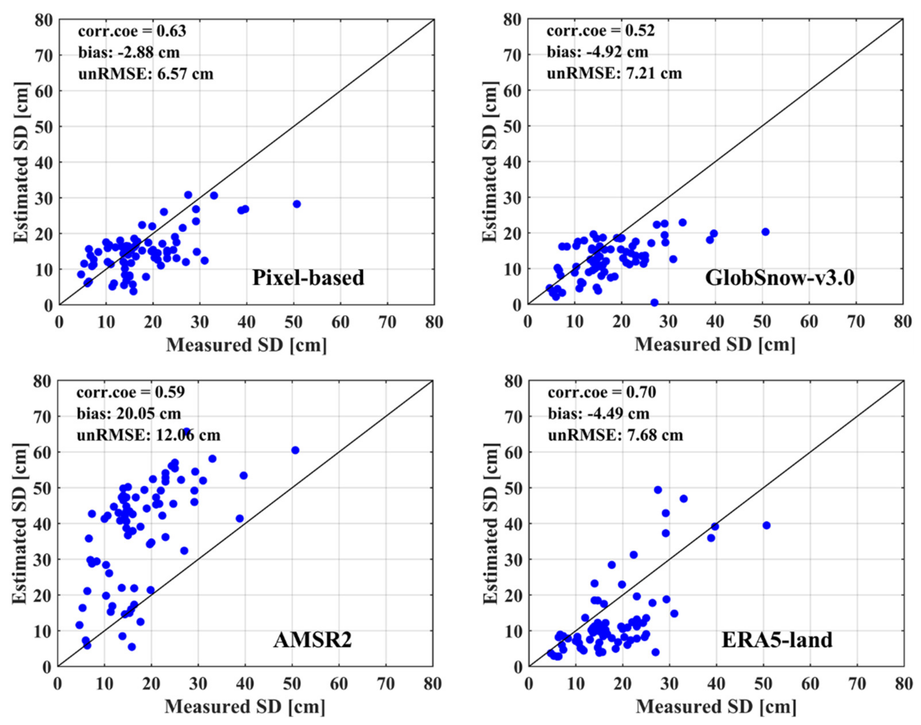
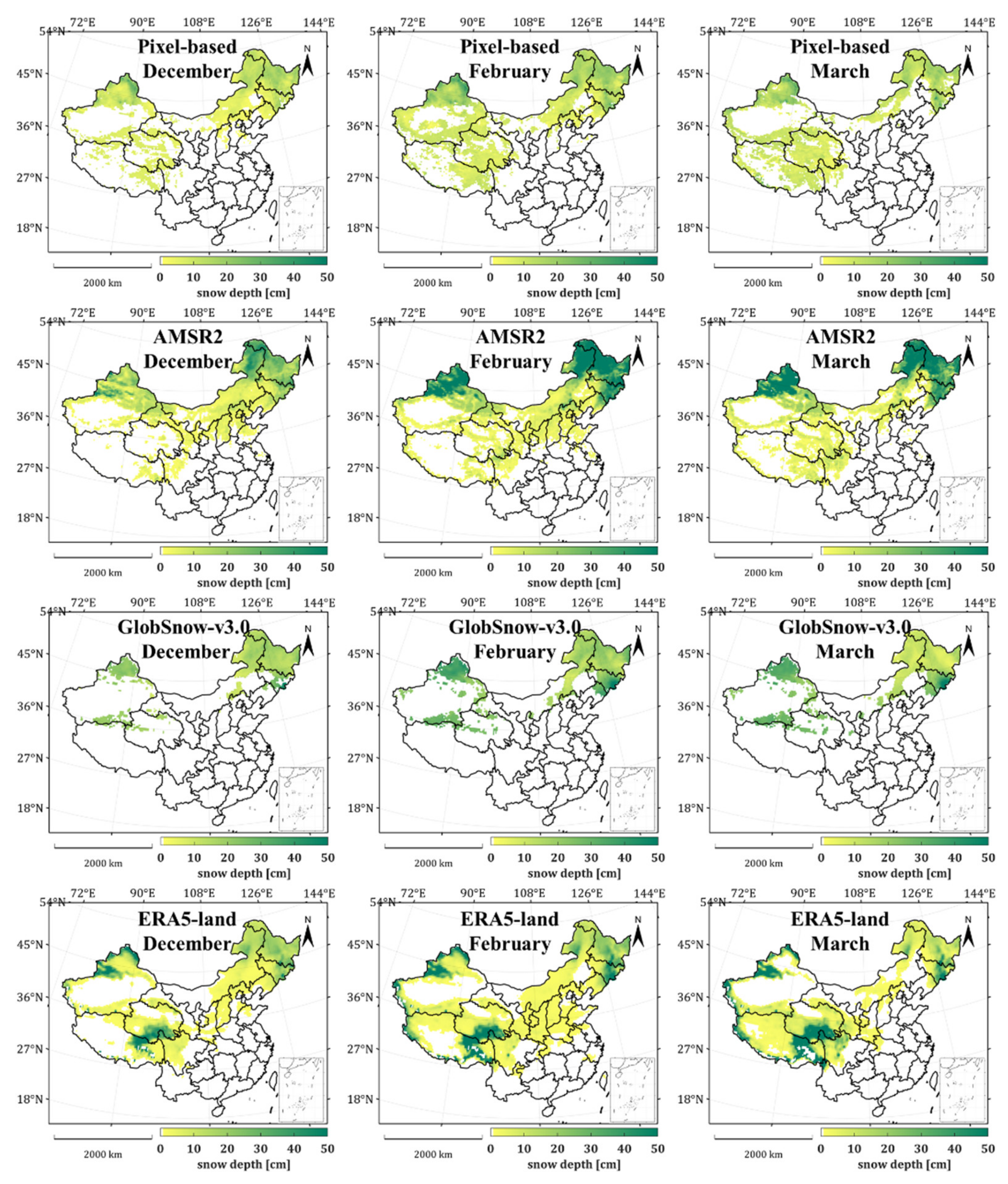
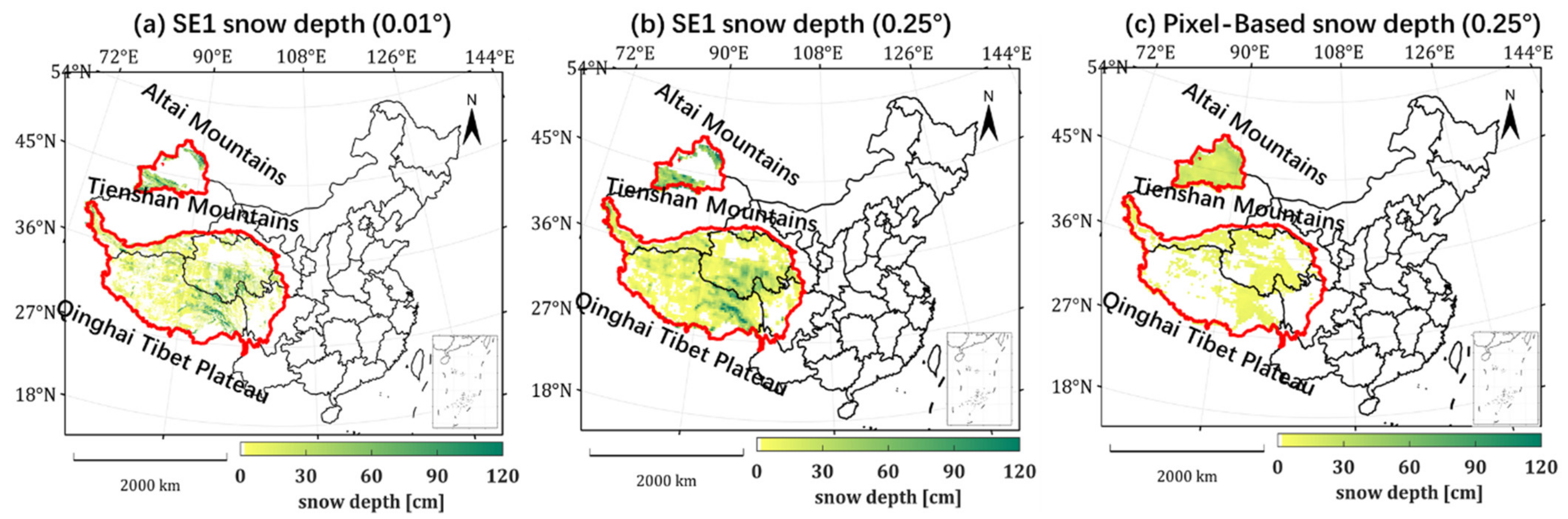
3.4. Evaluation of the Pixel-Based Algorithm and Comparison with Other Satellite Products
4. Discussion
5. Conclusions
Author Contributions
Funding
Data Availability Statement
Conflicts of Interest
References
- Barnett, T.P.; Adam, J.C.; Lettenmaier, D.P. Potential impacts of a warming climate on water availability in snow-dominated regions. Nature 2005, 438, 303–309. [Google Scholar] [CrossRef] [PubMed]
- Qin, Y.; Abatzoglou, J.T.; Siebert, S.; Huning, L.S.; AghaKouchak, A.; Mankin, J.S.; Hong, C.; Tong, D.; Davis, S.J.; Mueller, N.D. Agricultural risks from changing snowmelt. Nat. Clim. Chang. 2020, 10, 459–465. [Google Scholar] [CrossRef]
- Sturm, M.; Goldstein, M.; Parr, C. Water and life from snow: A trillion dollar science question. Water Resour. Res. 2017, 53, 3534–3544. [Google Scholar] [CrossRef]
- Pulliainen, J.; Luojus, K.; Derksen, C.; Mudryk, L.; Lemmetyinen, J.; Salminen, M.; Ikonen, J.; Takala, M.; Cohen, J.; Smolander, T.; et al. Patterns and trends of Northern Hemisphere snow mass from 1980 to 2018. Nature 2020, 581, 294–298. [Google Scholar] [CrossRef]
- Kraaijenbrink, P.; Stigter, E.; Yao, T.; Immerzeel, W.W. Climate change decisive for Asia’s snow meltwater supply. Nat. Clim. Chang. 2021, 11, 591–597. [Google Scholar] [CrossRef]
- Derksen, C.; Toose, P.; Rees, A.; Wang, L.; English, M.; Walker, A.; Sturm, M. Development of a tundra-specific snow water equivalent retrieval algorithm for satellite passive microwave data. Remote Sens. Environ. 2010, 114, 1699–1709. [Google Scholar] [CrossRef]
- Qu, X.; Hall, A. On the persistent spread in snow-albedo feedback. Clim. Dyn. 2014, 42, 69–81. [Google Scholar] [CrossRef]
- Tsang, L.; Durand, M.; Derksen, C.; Barros, A.P.; Kang, D.H.; Lievens, H.; Marshall, H.P.; Zhu, J.; Johnson, J.; King, J.; et al. Review Article: Global Monitoring of Snow Water Equivalent Using High Frequency Radar Remote Sensing. Cryosphere Discuss. 2021. in review. [Google Scholar] [CrossRef]
- Foster, J.L.; Sun, C.; Walker, J.P.; Kelly, R.; Chang, A.; Dong, J.; Powell, H. Quantifying the Uncertainty in Passive Microwave Snow Water Equivalent Observations. Remote Sens. Environ. 2005, 94, 187–203. [Google Scholar] [CrossRef]
- Saberi, N.; Kelly, R.; Flemming, M.; Li, Q. Review of snow water equivalent retrieval methods using spaceborne passive microwave radiometry. Int. J. Remote Sens. 2020, 41, 996–1018. [Google Scholar] [CrossRef]
- Chang, A.T.C.; Foster, J.L.; Hall, D.K. Nimbus-7 SMMR derived global snow cover parameters. Ann. Glaciol. 1987, 9, 39–44. [Google Scholar] [CrossRef]
- Derksen, C.; Walker, A.; Goodison, B. Evaluation of passive microwave snow water equivalent retrievals across the boreal forest tundra transition of western Canada. Remote Sens. Environ. 2005, 96, 315–327. [Google Scholar] [CrossRef]
- Che, T.; Li, X.; Jin, R.; Armstrong, R.; Zhang, T. Snow depth derived from passive microwave remote-sensing data in China. Ann. Glaciol. 2008, 49, 145–154. [Google Scholar] [CrossRef]
- Kelly, R. The AMSR-E Snow Depth Algorithm: Description and Initial Results. J. Remote Sens. Soc. Jpn. 2009, 29, 307–317. [Google Scholar]
- Jiang, L.; Wang, P.; Zhang, L.; Yang, H.; Yang, J. Improvement of snow depth retrieval for FY3B-MWRI in China. Sci. China Earth Sci. 2014, 44, 531–547. [Google Scholar] [CrossRef]
- Yang, J.; Jiang, L.; Wu, S.; Wang, G.; Wang, J.; Liu, X. Development of a Snow Depth Estimation Algorithm over China for the FY-3D/MWRI. Remote Sens. 2019, 11, 977. [Google Scholar] [CrossRef]
- Jiang, L.; Shi, J.; Tjuatja, S.; Dozier, J.; Chen, K.; Zhang, L. A parameterized multiple-scattering model for microwave emission from dry snow. Remote Sens. Environ. 2007, 111, 357–366. [Google Scholar] [CrossRef]
- Langlois, A.; Royer, A.; Derksen, C.; Montpetit, B.; Dupont, F.; Goïta, K. Coupling the snow thermodynamic model SNOWPACK with the microwave emission model of layered snowpacks for subarctic and arctic snow water equivalent retrievals. Water Resour. Res. 2012, 48, W12524. [Google Scholar] [CrossRef]
- Che, T.; Dai, L.; Zheng, X.; Li, X.; Zhao, K. Estimation of snow depth from passive microwave brightness temperature data in forest regions of northeast China. Remote Sens. Environ. 2016, 183, 334–349. [Google Scholar] [CrossRef]
- Picard, G.; Brucker, L.; Roy, A.; Dupont, F.; Fily, M.; Royer, A.; Harlow, C. Simulation of the microwave emission of multi-layered snowpacks using the dense media radiative transfer theory: The DMRT-ML model. Geosci. Model Dev. 2013, 6, 1061–1078. [Google Scholar] [CrossRef]
- Picard, G.; Sandells, M.; Löwe, H. SMRT: An active-passive microwave radiative transfer model for snow with multiple microstructure and scattering formulations (v1.0). Geosci. Model Dev. 2018, 11, 2763–2788. [Google Scholar] [CrossRef]
- Dai, L.; Che, T.; Wang, J.; Zhang, P. Snow depth and snow water equivalent estimation from AMSR-E data based on a priori snow characteristics in Xinjiang, China. Remote Sens. Environ. 2012, 127, 14–29. [Google Scholar] [CrossRef]
- Pan, J.; Durand, M.; Sandells, M.; Vander Jagt, B.; Liu, D. Application of a Markov Chain Monte Carlo algorithm for snow water equivalent retrieval from passive microwave measurements. Remote Sens. Environ. 2017, 192, 150–165. [Google Scholar] [CrossRef]
- Tedesco, M.; Jeyaratnam, J. A New Operational Snow Retrieval Algorithm Applied to Historical AMSR-E Brightness Temperatures. Remote Sens. 2016, 8, 1037. [Google Scholar] [CrossRef]
- Santi, E.; Brogioni, M.; Leduc-Leballeur, M.; Macelloni, G.; Montomoli, F.; Pampaloni, P.; Lemmetyinen, J.; Cohen, J.; Rott, H.; Nagler, T.; et al. Exploiting the ANN Potential in Estimating Snow Depth and Snow Water Equivalent from the Airborne SnowSAR Data at X- and Ku-Bands. IEEE Trans. Geosci. Remote Sens. 2021, 99, 1–16. [Google Scholar] [CrossRef]
- Bair, E.H.; Abreu Calfa, A.; Rittger, K.; Dozier, J. Using machine learning for real-time estimates of snow water equivalent in the watersheds of Afghanistan. Cryosphere 2018, 12, 1579–1594. [Google Scholar] [CrossRef]
- Xiao, X.; Zhang, T.; Zhong, X.; Shao, W.; Li, X. Support vector regression snow-depth retrieval algorithm using passive microwave remote sensing data. Remote Sens. Environ. 2018, 210, 48–64. [Google Scholar] [CrossRef]
- Wang, J.; Forman, B.A.; Xue, Y. Exploration of synthetic terrestrial snow mass estimation via assimilation of amsr-e brightness temperature spectral differences using the catchment land surface model and support vector machine regression. Water Resour. Res. 2020, e2020WR027490. [Google Scholar] [CrossRef]
- Yang, J.; Jiang, L.; Luojus, K.; Pan, J.; Lemmetyinen, J.; Takala, M.; Wu, S. Snow depth estimation and historical data reconstruction over China based on a random forest machine learning approach. Cryosphere 2020, 14, 1763–1778. [Google Scholar] [CrossRef]
- Yang, J.; Jiang, L.; Lemmetyinen, J.; Pan, J.; Luojus, K.; Takala, M. Improving snow depth estimation by coupling HUT-optimized effective snow grain size parameters with the random forest approach. Remote Sens. Environ. 2021, 264, 112630. [Google Scholar] [CrossRef]
- Che, T.; Li, X.; Jin, R.; Huang, C. Assimilating passive microwave remote sensing data into a land surface model to improve the estimation of snow depth. Remote Sens. Environ. 2014, 143, 54–63. [Google Scholar] [CrossRef]
- Li, D.; Durand, M.; Margulis, S. Estimating snow water equivalent in a Sierra Nevada watershed via spaceborne radiance data assimilation. Water Resour. Res. 2017, 53, 647–741. [Google Scholar] [CrossRef]
- Xue, Y.; Forman, B.A.; Reichle, R.H. Estimating snow mass in North America through assimilation of Advanced Microwave Scanning Radiometer brightness temperature observations using the Catchment land surface model and support vector machines. Water Resour. Res. 2018, 54, 6488–6509. [Google Scholar] [CrossRef] [PubMed]
- Larue, F.; Royer, A.; De Sève, D.; Roy, A.; Picard, G.; Vionnet, V.; Cosme, E. Simulation and assimilation of passive microwave data using a snowpack model coupled to a well-calibrated radiative transfer model over North-Eastern Canada. Water Resour. Res. 2018, 54, 1–26. [Google Scholar] [CrossRef]
- Merkouriadi, I.; Lemmetyinen, J.; Liston, G.E.; Pulliainen, J. Solving Challenges of Assimilating Microwave Remote Sensing Signatures with a Physical Model to Estimate Snow Water Equivalent. Water Resour. Res. 2021, 57, 1–24. [Google Scholar] [CrossRef]
- Kim, R.S.; Durand, M.; Li, D.; Baldo, E.; Margulis, S.A.; Dumont, M.; Morin, S. Estimating alpine snow depth by combining multifrequency passive radiance observations with ensemble snowpack modeling. Remote Sens. Environ. 2019, 226, 1–15. [Google Scholar] [CrossRef]
- Xiong, C.; Shi, J.; Pan, J.; Xu, H.; Che, T.; Zhao, T.; Ren, Y.; Geng, D.; Chen, T.; Jiang, K.; et al. Time Series X- and Ku-Band Ground-Based Synthetic Aperture Radar Observation of Snow-Covered Soil and Its Electromagnetic Modeling. IEEE Trans. Geosci. Remote Sens. 2022, 60, 1–13. [Google Scholar] [CrossRef]
- Lemmetyinen, J.; Derksen, C.; Toose, P.; Proksch, M.; Pulliainen, J.; Kontu, A.; Hallikainen, M. Simulating seasonally and spatially varying snow cover brightness temperature using HUT snow emission model and retrieval of a microwave effective grain size. Remote Sens. Environ. 2015, 156, 71–95. [Google Scholar] [CrossRef]
- Xue, Y.; Forman, B.A. Atmospheric and Forest Decoupling of Passive Microwave Brightness Temperature Observations Over Snow-Covered Terrain in North America. IEEE J. Select. Top. Appl. Earth Observ. Remote Sens. 2017, 10, 3172–3189. [Google Scholar] [CrossRef]
- Li, Q.; Kelly, R.; Leppanen, L.; Juho, V.; Kontu, A.; Lemmetyinen, J.; Pulliainen, J. The Influence of Thermal Properties and Canopy-Intercepted Snow on Passive Microwave Transmissivity of a Scots Pine. IEEE Trans. Geosci. Remote Sens. 2019, 99, 1–10. [Google Scholar] [CrossRef]
- Li, Q.; Kelly, R.; Lemmetyinen, J.; Roo, R.D.D.; Pan, J.; Qiu, Y. The influence of tree transmissivity variations in winter on satellite snow parameter observations. Int. J. Digit. Earth 2021, 14, 1337–1353. [Google Scholar] [CrossRef]
- Venäläinen, P.; Luojus, K.; Lemmetyinen, J.; Pulliainen, J.; Moisander, M.; Takala, M. Impact of dynamic snow density on GlobSnow snow water equivalent retrieval accuracy. Cryosphere 2021, 15, 2969–2981. [Google Scholar] [CrossRef]
- Reichstein, M.; Camps-Valls, G.; Stevens, B.; Jung, M.; Denzler, J.; Carvalhais, N.; Prabhat. Deep learning and process understanding for data-driven Earth system science. Nature 2019, 566, 195–204. [Google Scholar] [CrossRef]
- Tedesco, M.; Jeyaratnam, J.; Kelly, R. NRT AMSR2 Daily L3 Global Snow Water Equivalent EASE-Grids; NASA LANCE AMSR2 at the Global Hydrology Resource Center Distributed Active Archive Center: Huntsville, AL, USA, 2015. [Google Scholar]
- Luojus, K.; Pulliainen, J.; Takala, M.; Lemmetyinen, J.; Mortimer, C.; Derksen, C.; Mudryk, L.; Moisander, M.; Hiltunen, M.; Smolander, T.; et al. GlobSnow v3.0 Northern Hemisphere snow water equivalent dataset. Sci. Data 2021, 8, 163. [Google Scholar] [CrossRef] [PubMed]
- Breiman, L. Random forests. Mach. Learn. 2001, 45, 5–32. [Google Scholar] [CrossRef]
- Cortes, C.; Vapnik, V.; Saitta, L. Support-Vector Networks Editor. Mach. Learn. 1995, 20, 273–297. [Google Scholar] [CrossRef]
- Vapnik, V.; Golowich, S.E.; Smola, A.J. Support vector method for function approximation, regression estimation and signal processing. Adv. Neural Inf. Processing Syst. 1997, 7, 281–287. [Google Scholar]
- Liu, H.; Li, Q.; Bai, Y.; Yang, C.; Wu, G. Improving satellite retrieval of oceanic particulate organic carbon concentrations using machine learning methods. Remote Sens. Environ. 2021, 256, 112316. [Google Scholar] [CrossRef]
- Specht, D.F. A general regression neural network. IEEE Trans. Neural Netw. 1991, 2, 568–576. [Google Scholar] [CrossRef]
- Basheer, I.; Hajmeer, M. Artificial neural networks: Fundamentals, computing, design, and application. J. Microbiol. Methods 2000, 43, 3–31. [Google Scholar] [CrossRef]
- Dobreva, I.; Klein, A. Fractional snow cover mapping through artificial neural network analysis of modis surface reflectance. Remote Sens. Environ. 2011, 115, 3355–3366. [Google Scholar] [CrossRef]
- Broxton, P.; van Leeuwen, W.; Biederman, J. Improving snow water equivalent maps with machine learning of snow survey and lidar measurements. Water Resour. Res. 2019, 55, 3739–3757. [Google Scholar] [CrossRef]
- Tarpanelli, A.; Santi, E.; Tourian, M.; Filippucci, P.; Amarnath, G.; Brocca, L. Daily river discharge estimates by merging satellite optical sensors and radar altimetry through artificial neural network. IEEE Trans. Geosci. Remote Sens. 2019, 57, 329–341. [Google Scholar] [CrossRef]
- Takala, M.; Luojus, K.; Pulliainen, J.; Lemmetyinen, J.; Juha-Petri, K.; Koskinen, J.; Bojkov, B. Estimating northern hemisphere snow water equivalent for climate research through assimilation of space-borne radiometer data and ground-based measurements. Remote Sens. Environ. 2011, 115, 3517–3529. [Google Scholar] [CrossRef]
- Li, X.J.; Liu, Y.J.; Zhu, X.X.; Zheng, Z.J.; Chen, A.J. Snow Cover Identification with SSM/I Data in China. J. Appl. Meteorol. Sci. 2007, 18, 12–20. [Google Scholar]
- Dozier, J.; Bair, E.; Davis, R. Estimating the spatial distribution of snow water equivalent in the world’s mountains. WIREs Water 2016, 3, 461–474. [Google Scholar] [CrossRef]
- Lievens, H.; Demuzere, M.; Marshall, H.P.; Reichle, R.H.; Brucker, L.; Brangers, I.; de Rosnay, P.; Dumont, M.; Girotto, M.; Immerzeel, W.W.; et al. Snow depth variability in the Northern Hemisphere mountains observed from space. Nat Commun. 2019, 10, 4629. [Google Scholar] [CrossRef]
- Lievens, H.; Brangers, I.; Marshall, H.P.; Jonas, T.; Olefs, M.; De Lannoy, G. Sentinel-1 snow depth retrieval at sub-kilometer resolution over the European Alps. Cryosphere 2022, 16, 159–177. [Google Scholar] [CrossRef]
- Painter, T.; Berisford, D.; Boardman, J.; Bormann, K.; Deems, J.; Gehrke, F. The Airborne Snow Observatory: Fusion of scanning lidar, imaging spectrometer, and physically-based modeling for mapping snow water equivalent and snow albedo. Remote Sens. Environ. 2016, 184, 139–152. [Google Scholar] [CrossRef]
- Royer, A.; Roy, A.; Jutras, S.; Langlois, A. Performance assessment of radiation-based field sensors for monitoring the water equivalent of snow cover (SWE). Cryosphere 2021, 15, 5079–5098. [Google Scholar] [CrossRef]
- Treichler, D.; Kääb, A. Snow depth from ICESat laser altimetry-a test study in southern norway. Remote Sens. Environ. 2017, 191, 389–401. [Google Scholar] [CrossRef]


| Data Product | Initial Resolution | Post Processing | Final Resolution | Reference/Availability |
|---|---|---|---|---|
| AMSR2 | 0.25° × 0.25° (daily) | \ | 0.25° × 0.25° (daily) | http://gportal.jaxa.jp/gpr/ (accessed on 25 May 2020) |
| GlobSnow-v3.0 | 25 km × 25 km (daily) | linear resampling | https://www.globsnow.info/ (accessed on 1 March 2022) | |
| ERA5-land | 0.1° × 0.1° (hourly) | linear resampling | https://cds.climate.copernicus.eu/ (accessed on 28 May 2020) |
| Predictor Variables | Interpretation | Source | Target Variable |
|---|---|---|---|
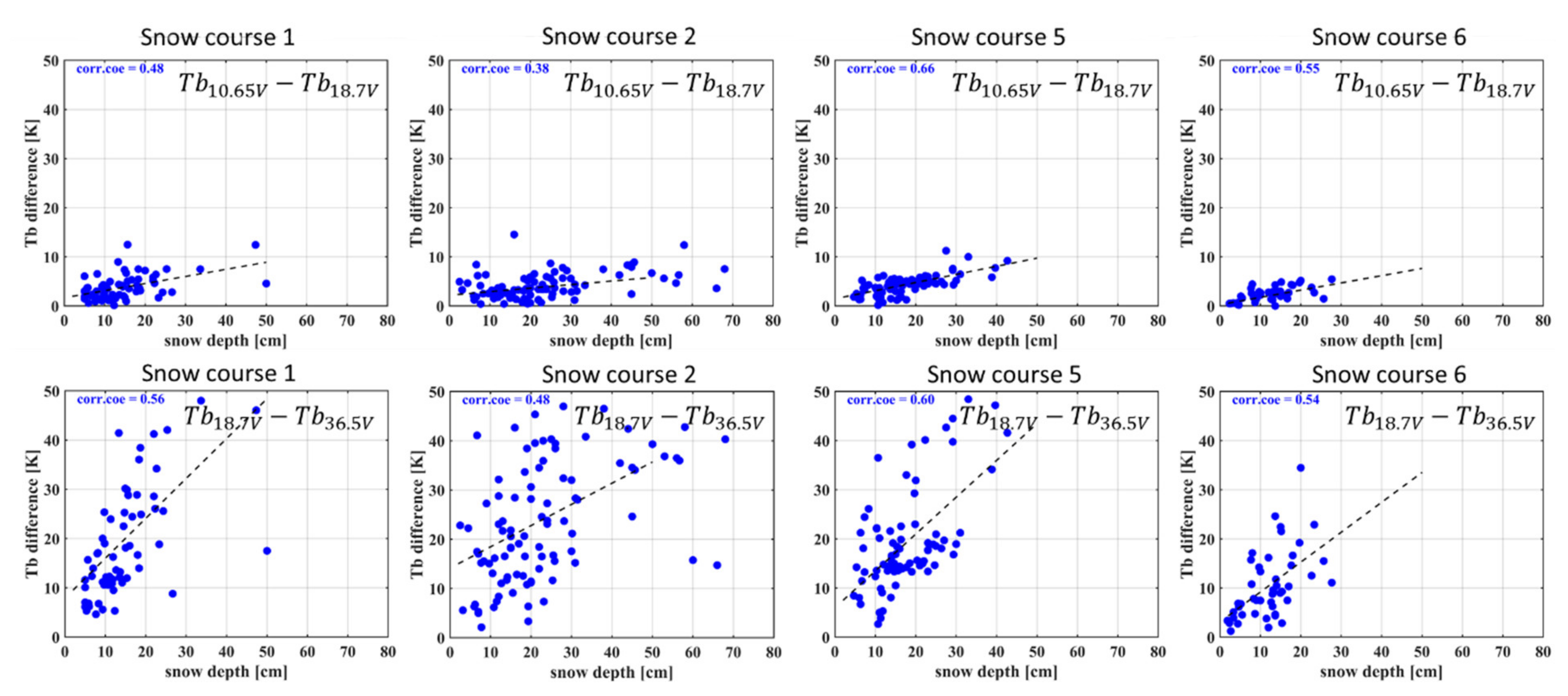
| Tb10.65V − Tb36.5V | vertical polarized spectral difference at 10.65 GHz and 36.5 GHz | AMSR2 | Snow depth in centimeters (weather station, 2012–2020) |
| Tb18.7V − Tb36.5V | vertical polarized spectral difference at 18.7 GHz and 36.5 GHz | AMSR2 | |
| Elevation | altitude in meters | weather station | |
| Longitude | longitude in degrees | weather station | |
| EffGS | effective grain size in millimeters | optimized by HUT |
Publisher’s Note: MDPI stays neutral with regard to jurisdictional claims in published maps and institutional affiliations. |
© 2022 by the authors. Licensee MDPI, Basel, Switzerland. This article is an open access article distributed under the terms and conditions of the Creative Commons Attribution (CC BY) license (https://creativecommons.org/licenses/by/4.0/).
Share and Cite
Yang, J.; Jiang, L.; Pan, J.; Shi, J.; Wu, S.; Wang, J.; Pan, F. Comparison of Machine Learning-Based Snow Depth Estimates and Development of a New Operational Retrieval Algorithm over China. Remote Sens. 2022, 14, 2800. https://doi.org/10.3390/rs14122800
Yang J, Jiang L, Pan J, Shi J, Wu S, Wang J, Pan F. Comparison of Machine Learning-Based Snow Depth Estimates and Development of a New Operational Retrieval Algorithm over China. Remote Sensing. 2022; 14(12):2800. https://doi.org/10.3390/rs14122800
Chicago/Turabian StyleYang, Jianwei, Lingmei Jiang, Jinmei Pan, Jiancheng Shi, Shengli Wu, Jian Wang, and Fangbo Pan. 2022. "Comparison of Machine Learning-Based Snow Depth Estimates and Development of a New Operational Retrieval Algorithm over China" Remote Sensing 14, no. 12: 2800. https://doi.org/10.3390/rs14122800
APA StyleYang, J., Jiang, L., Pan, J., Shi, J., Wu, S., Wang, J., & Pan, F. (2022). Comparison of Machine Learning-Based Snow Depth Estimates and Development of a New Operational Retrieval Algorithm over China. Remote Sensing, 14(12), 2800. https://doi.org/10.3390/rs14122800