Abstract
The orientation of satellite images is a necessary operation for the correct geometric use of satellite images whether they are used individually to obtain an orthophoto or as stereocouples to extract three-dimensional information. The orientation allows us to reconstruct the correct position on the ground of the single pixels that form the image, which normally can be performed using certain functions of commercial software customised for each specific satellite. These functions read the metadata parameters provided by the satellite operator and use them to correctly orient the images. Unfortunately, these parameters have not been standardised and various satellites report them according to variable conventions, so new satellites or those that are not widely used cannot be oriented automatically. The PRISMA satellite launched by the Italian Space Agency (ASI) releases free hyperspectral and panchromatic images with metric resolution, but there is not yet a standardised procedure for orienting its images and this limits its usability. This paper reports on the first experimentation of orientation and orthorectification of PRISMA (PRecursore IperSpettrale della Missione Applicativa) images carried out using the three most widely used models, namely the rigorous, the Rational Polynomial Coefficients (RPC) and the Rational Polynomial Functions (RPF) tools. The results obtained by interpreting the parameters and making them suitable for use in standard procedures have made it possible to obtain results with an accuracy equal to the maximum resolution of panchromatic images (5 m), thus making it possible to achieve the highest level of geometric accuracy that can be extracted from the images themselves.
1. Introduction
In the last twenty years, many satellite missions dedicated to earth observation have become operational. As a result, on-board technologically advanced sensors have allowed for the acquisition of panchromatic and multispectral images with, respectively, sub-metric and metric resolutions. The applications of such images cover a very wide and continuously evolving field of application from automatic feature extraction [1] to landslide monitoring [2,3] and image classification [4]. In all applications, geometric accuracy is of particular importance, especially in cases where positional comparability determines the final accuracy, as in the case of cartography updates or change detection analyses [5]. Nowadays, the available products have a wide range of spatial resolutions, while, with regard to the spectral resolution, hyperspectral satellites are still poorly represented in spaceborne missions compared to multispectral ones [6].
In March 2019, the Italian Space Agency (ASI) launched a new satellite named “PRISMA” (PRecursore IperSpettrale della Missione Applicativa) equipped with hyperspectral and medium resolution panchromatic sensors [7,8,9]. Specifically, the spatial resolution of panchromatic product is 5 m, while the hyperspectral sensor acquires scenes with a Ground Sampling Distance (GSD) of 30 m in the spectral range between 400 and 2500 nm with 10 nm spectral sampling.
It is important to note that PRISMA satellite is, in the current panorama, a unique platform of its kind as it combines the possibilities of hyperspectral sensors with those of panchromatic sensors, thereby promoting a more detailed analysis and a more precise detection of the ground features. The only commonly known satellite platform with similar characteristics is the EO-1 Hyperion/ALI, which had a lower resolution for panchromatic data (10 metres) and is currently (as of 2017) no longer operational. The open and free availability of the images for the scientific community, both for archival and new acquisitions images, makes the study of the PRISMA sensor even more interesting for the world of research.
This mission offers a new opportunity for environmental monitoring in cases such as forest analysis and water application [10,11]. Considering the newness of the mission, the studies conducted so far have focused on possible hyperspectral applications, using already georeferenced data; however, it is necessary to verify the accuracy of geolocation [12]. In fact, the hyperspectral and panchromatic PRISMA products are currently available with a declared geolocation accuracy of 200 m, which ASI plans to increase to half a pixel in the near future by introducing geometric correction of the images with Ground Control Points (GCPs).
Apart from the application used, satellite images are affected by deformation mainly due to camera distortions and acquisition geometry, after which they must undergo a geometric rectification process in order to define the precision and accuracy level, this process is known as orthorectification.
Geometric rectification is performed by describing the relationship between image and ground coordinates with the following approaches: with the empirical or photogrammetric-based model [13,14]. Usually, the orthorectification includes the following two processes: first, the orientation parameters are estimated by using GCP with the aim to reconstruct the acquisition characteristic (sensor’s attitude, position and internal parameters), then the oriented images are projected after considering a DEM or DSM.
At present, orientation methods can be classified into the following three categories: empirical methodologies, such as Rational Polynomial Functions—RPFs, that are independent of specific platform or sensor characteristics and acquisition geometry; physically based models that follow a photogrammetric approach (rigorous model), which takes into account several aspects influencing the acquisition procedure; a third type of model that represents a compromise between the first two, RPC—Rational Polynomial Coefficients models, in which the RPF approach is used with known coefficients supplied in the imagery metadata and “blind” produced by companies managing sensors with their own rigorous models. The RPC approach results may be enhanced by users estimating some additional parameters (e.g., an affine transform) on the basis of eventually available GCPs [15,16,17,18].
The different orthorectification approaches have been extensively tested on the most popular satellite platforms outlining the advantages and disadvantages of the various approaches in a consolidated way, therefore the results obtained with PRISMA must be considered in relation to the state of the art that is well documented in the literature for most other platforms.
The rigorous model reconstructs the reality of the acquisition geometry starting from the satellite platform information, such as satellite ephemeris and attitude and sensor and image characteristics; therefore, such models prove to be specific for each satellite system and produce results that are more robust with respect to the RPF empirical model. Furthermore, with RPF the geometric correction is applied locally and conditioned by the GCP distribution and number.
Nowadays, the third type of model, the RPC, represents an interesting and attractive solution to orienting satellite images, as it can apply geometric correction with a good level of accuracy, which in some cases is comparable with the rigorous model, using fewer GCPs than the RPF model. Finally, this type of model is supported by almost all commercial and free software and it is independent of the sensor characteristics [10,19,20,21].
Geometric correction is a fundamental step that affects all subsequent forms of processing of the image itself and the accuracy of the final product strictly depends on the original image characteristics, on the quality of the known coordinates of ground control points and on the model chosen to perform the orientation. Satellite image processing methods and the analysis of precision and accuracy of derived products are widely investigated [22,23,24,25,26,27].
However, the PRISMA satellite has specific characteristics and problems that make simple orientation and orthorectification complex, if not impossible for non-expert users, significantly limiting the application possibilities of an otherwise very interesting platform. In the present work, a specific procedure has been developed on the basis of the experience and state of the art of other platforms to solve specific problems of PRISMA never previously observed on other satellites. As a result of experimentation we were able to define and verify certain procedures that provide a correct orientation of PRISMA images even for users who are not experts in the photogrammetric aspect. Presently, there are no other scientific contributions on the specific problem of the orthorectification of PRISMA images.
Nowadays, the main commercial software implements all three models, but it does not yet provide processing with rigorous approaches or RPCs for PRISMA images, probably due to the recent availability of these products.
When a new sensor is not supported by commercial software, such as PCI-Geomatica OrthoEngine, the function Read Generic Image File can be used, which provides the image orientation using a photogrammetric approach only if the user manually enters information about the orbit and acquisition characteristics.
This approach was also applied to PRISMA but the results are limited due to the scarce official data available for the specific platform.
2. Materials and Methods
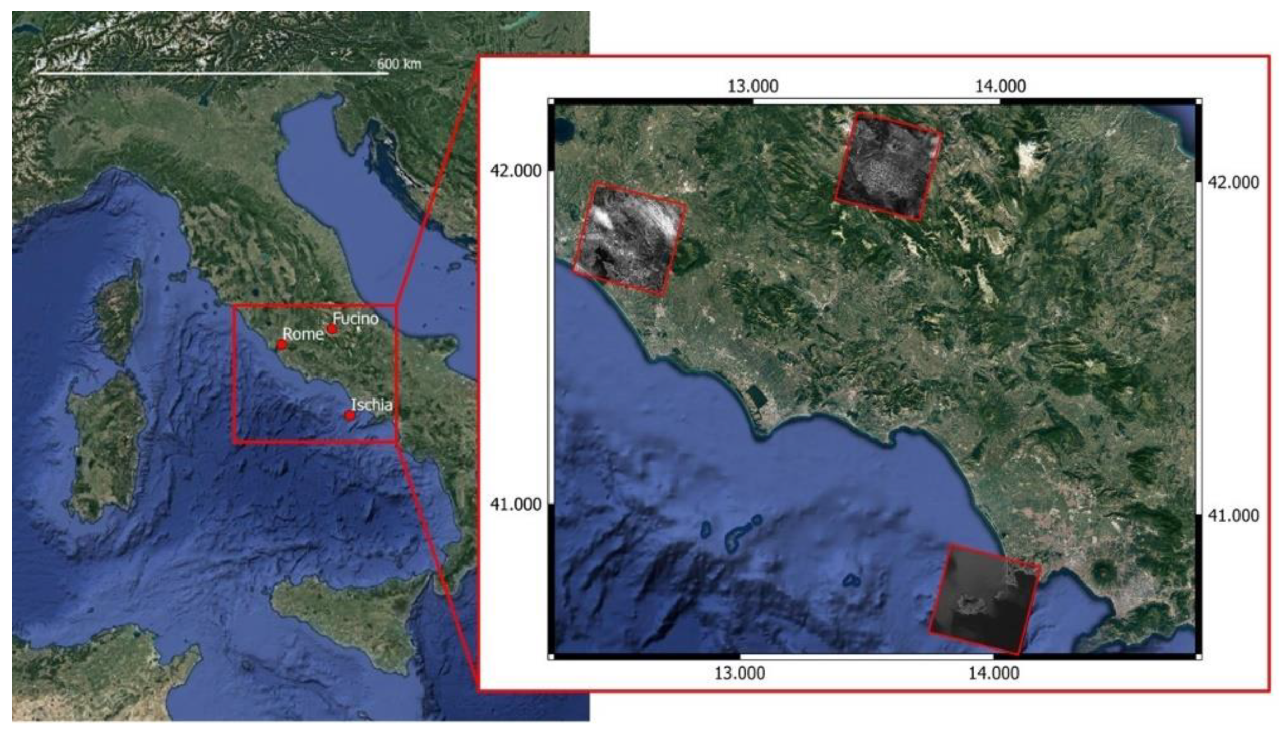
Geometric correction of the PRISMA panchromatic products was performed by considering three images (Figure 1) representing morphologically different areas, since the altimetric aspect characterizes the orthorectification process. The panchromatic images processed are 30 km × 30 km in size and include both catalogue products and new acquisitions. Table 1 shows the main characteristics of the images analysed.

Figure 1.
Location of the three test fields.

Table 1.
Main features of PRISMA images.
The first test field covers a central area of the city of Rome, which is rich in urban elements facilitating the identification of GCPs. In particular, large, historical buildings are essential elements because they are clearly recognizable even on panchromatic products with a medium spatial resolution such as PRSIMA images. The GCPs were collimated homogeneously on the image as accurately as possible given the presence of a modest partial cloud cover. The coordinates of GCPs were obtained from vector cartography at a scale of 1:5000 provided by the Lazio Region portal (http://dati.lazio.it, accessed on 22 February 2022), while the altimetric information was obtained from the digital terrain model (DEM) in orthometric elevations with TINITALY/01 provided by INGV [28] and a resolution of 10 m per pixel. This DEM was selected because its resolution is adequate for the orthorectification of an image with a resolution of 5 m; other DEMs with a higher resolution are available (e.g., from maps at a scale of 1:5000), but, in our opinion, they would have unnecessarily burdened the processing.
The second test field covers the Fucino plain (Abruzzo region, Italy), a morphologically depressed structure surrounded by major mountain reliefs. This area represents an interesting test field due to the particular altimetric-geomorphological condition, characterised by rapid altimetric variations in the correspondence of reliefs which cover the entire perimeter of the image. In this case, GCP identification is more complex because the plain is mainly agricultural and therefore lacks easily recognisable urban elements. For this reason, the crossroads of the plain and the small buildings distributed among the cultivated fields were used. The GCP coordinates for the Fucino image were obtained using vector cartography with a scale of 1:5000 and the digital terrain model, both provided by the web page of the Abruzzo Region administration (http://opendata.regione.abruzzo.it/, accessed on 22 February 2022).
The last test field is the isle of Ischia (Campania Region, Italy), which covers only a partial area (approximately 10 km E-W × 8 km N-S) of the acquired image. This choice is justified by the particular morphological condition of the island, surmounted by Mount Epomeo at 789 m above sea level. GCP identification was complex due to the presence of irregular settlements and a road network that conforms to the complexity of the territory. Despite these difficulties and the spatial resolution at 5 m, enough GCPs were identified, whose coordinates and elevations were obtained from the vector cartography at a scale of 1:2000, provided by the Metropolitan City of Naples; furthermore, the digital terrain model, with 1 m resolution, was obtained from regional cartography.
2.1. Export Procedure for Specific Bands and Related Issues
PRISMA products are provided at different processing levels and are widely described in the literature [7]. Their differences mainly concern the hyperspectral data. In the present experimentation, panchromatic products of L2C level, i.e., “geolocated and geocoded atmospherically corrected HYP and PAN images”, were used. Specifically, the geolocation process of the PRISMA products consists of the estimation of the orientation model based on the Line of Sight, without the use of DEM and GCPs. In order to improve the geometric accuracy, the model parameters could be refined using an automatic method of GCPs searching; currently, this phase has not yet been performed, so the geolocation information was released with approximate accuracy (200 m) in the form of Rational Function Model (RFM). The RFM model is applied to L2D products, providing orthorectified ground reflectance images, while in L2C products it is only attached as metadata information. For our purposes, we selected L2C products, as the images are available in raw matrix form and RPC coefficients can be derived from metadata, allowing users to perform an independent geometric correction to achieve higher geometric accuracy.
The PRISMA products are released in an HDF-EOS5 format, then to export the panchromatic data in GeoTIFF format several solutions have been tested, including the following: ENVI software (from version 5.5.3 it supports the PRISMA data), Erdas Imagine, the open-source software QGis, the “prismaread” method accessible from R [12] and MATLAB. In the data export phase, it is important to ensure that the raster has not undergone any preliminary geocoding, since this would return altered data incongruent with the “Geocoding Model” parameters provided. To verify the absence of geocoding, the extracted data can be imported into any GIS software to verify that the graphic restitution of the raster corresponds to its matrix coordinates (internal coordinate reference system), that is, the coordinates of the top-left corner must be 0, 0.
The geocoding model information (PRISMA Products Specification Document) is contained in the metadata but it is not attached to the exported GeoTIFF product and, as a consequence, it was attached by means of a text file in the RPC00B format. In fact, as reported in the documentation, the geocoding model adopted for L2 products is the Rational Polynomial Coefficient model: RPC00B—Rapid Positioning Capability, as defined in the National Imagery and Mapping Agency standard [29]. For PRISMA panchromatic products, the matrix dimension is a 6000 × 6000 pixel, without any projection.
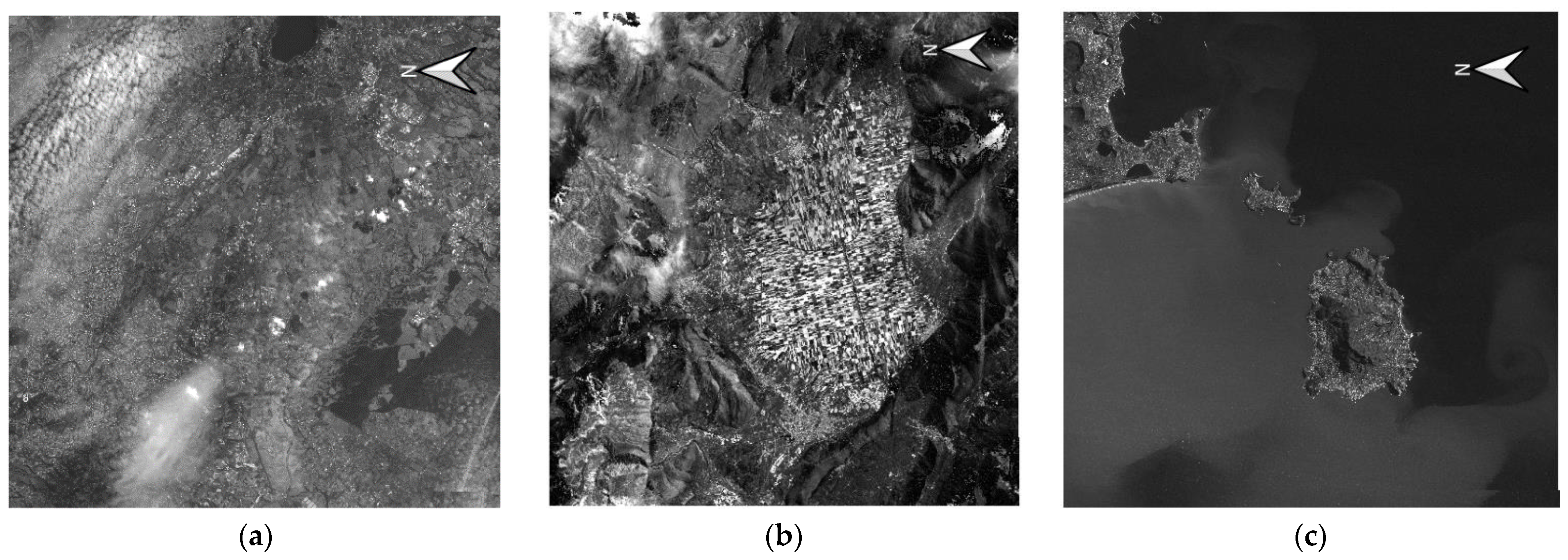
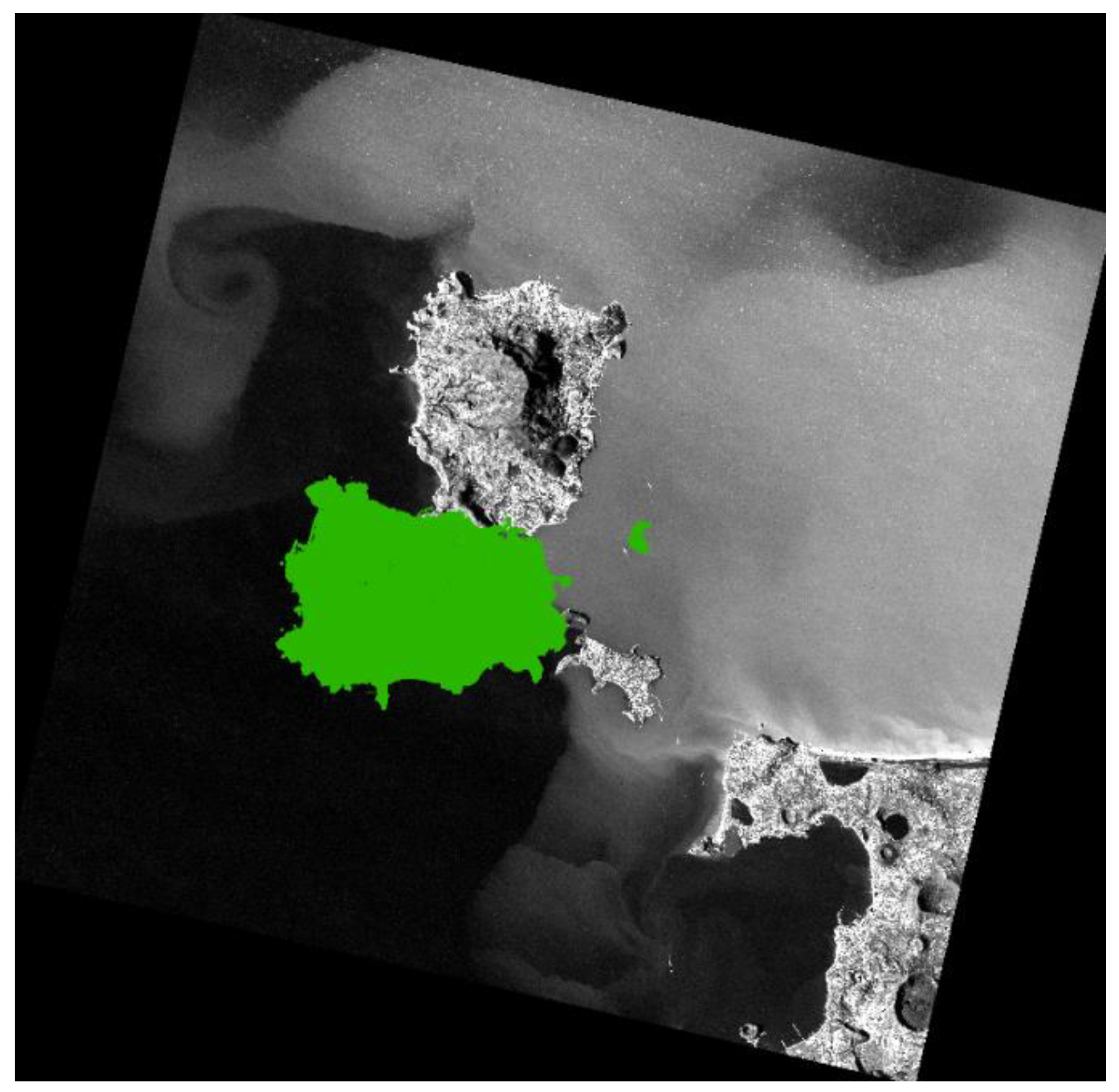
A fundamental aspect for the correct application of polynomial rational coefficients is the export of raw data, which is presented with the North direction rotated 90° counterclockwise (Figure 2). The application of RPCs to exported raw images that are correctly oriented North produced final orthorectified images that are rotated with respect to the real geographic position, as shown in Figure 3, where the orthorectified image presents a wrong rotation with respect to the Isle of Ischia (in green).

Figure 2.
Correct export of the panchromatic product, test field of Rome (a), Fucino (b) and Ischia (c).

Figure 3.
Superimposition between the “orthorectified” image, obtained using a north-correct raw image, and the actual position of the isle of Ischia (in green).
2.2. Orthorectification of PRISMA Images
The photogrammetric processing of pushbroom satellite images is usually based on the application of the following three methods: the rigorous approach and the polynomial function method with RPCs provided with the image or estimated image on the basis of a large set of GCPs. In this experimentation, we tried to test all three methods to provide a broader view of the geometric elaboration of PRISMA images.
Currently, a specific rigorous model for PRISMA images has not yet been implemented, only the commercial software OrthoEngine provides a function, named “Read Generic Image File”, that can reconstruct the orbital parameters starting from information available in the metadata file. Only a few tests have been carried out using the function “Read Generic Image File” because some information (such as information related to the across-track and along-track angles) is not provided in the format required and documentation with an explanation of the parameter’s physical meaning is still unavailable [19].
For this reason, the authors believe that the experimentation of the rigorous model reported below should be considered preliminary due to the uncertainties mentioned regarding the validity of the orbital parameters used (some of which were estimated before launch) and the interpretation of them. Unfortunately, these uncertainties also depend on the known lack of standardisation of the orbital and orientation parameters already observed in previous works in the literature [19].
Therefore, the authors underline that the experiments must be viewed as garnering the best result currently achievable with the data and means that could be found, but they are open to advice and suggestions from the scientific community.
The results obtained with the RPF and RPC models have instead been widely analysed.
The RPF empirical model is generally based on third-degree polynomials that relate an object and image coordinates, using 78 rational polynomial coefficients estimated with a least-square process based on an adequate number of GCPs. The RPF model can be given as:
where aj, bj, cj, dj are the polynomial coefficients, I and J are the image coordinates and λ, φ, h are the corresponding object point coordinates. The RPC model is based on the RPF approach, but the coefficients are known and supplied in the imagery metadata. An RPC model with third-order polynomials, in the format RPC00B, is generally used, but the order of the terms may differ for different applications [29]. The orientation given by RPCs can be improved by estimating the parameters of a polynomial transformation on the basis of a set of GCPs; the polynomial order can vary from 0 to 2 [17]. Table 2 shows the strictly necessary GCP number for parameter estimation, but in our elaboration, several redundancy conditions have been achieved to reduce the risk of errors due to outliers or a strong dependence on the chosen GCPs.
Table 2.
Parameters and minimum GCP numbers for RPC refinement in OrthoEngine.
The PRISMA Geocoding Model data include the RPC coefficients and parameters for normalizing the row, column, latitude, longitude and ellipsoidal height values. The parameters provided together with PRISMA imagery comply with NIMA standards, but they include a total of only 40 non-zero coefficients, which are sufficient only for the calculation of second order rational polynomials. Moreover, the Geocoding Model parameters are extracted from metadata and transcribed into a file with the “RPB” extension, following the RPB00B format, in order to create the standard format for processing in the most commonly used software.
RPC and RFP models were performed with OrthoEngine software and an extensive analysis was conducted.
For the application of the RPC model, 20 points were collimated for each image; initially all of them were set as Check Points (CPs) for the estimation of the geopositioning accuracy given only by the application of the RPC provided; progressively some points were chosen as GCPs for the estimation of refinement parameters. Several tests have been performed on each image, by increasing the number of GCPs used for orientation parameters estimation, starting from 2 GCPs and 18 CPs, up to a configuration with 10 GCPs and 10 CPs. The RMSE values for each test, for each test field and for each transformation starting from order 0, up to order 2, are reported.
The RPF method has been applied on all test fields and a total of 60 points for each image have been collimated: 47 used as GCPs for coefficients estimation and 13 used as CPs for validation of the oriented image.
3. Results and Discussion
The experiments conducted on the three field tests (Rome, Ischia Island and Fucino) were replicated using the following three models: rigorous, RPC and RPF. All the results are reported below except for some results from tests with the RPC model, which are reported in the Appendix A for completeness but which are not reported here in the main text because they do not provide exhaustive results and so were deemed to unnecessarily burden the text.
3.1. Rigorous Model
3.1.1. Results of Rigorous Model
The “Read Generic Image File” function available in OrthoEngine software allows for the creation of an orbital model for image formats, whose ephemeris data are not read automatically by the software itself, usually because the satellite has just been released as in the case under study. This function allows for the satellite image and orbit information to be entered manually. Table 3 shows the parameters that are required by the application and the orbital and sensor information includes the IFOV, flight height, orbit period and inclination, and eccentricity; for the PRISMA product, this information is derived from pre-launch data available in the literature [30,31,32]. Unfortunately, the across-track angle, i.e., the angle between the vertical and the observation direction during the side scan, and the along-track angle, i.e., the angle between the vertical and the forward or backward observation direction, are different for each image and they are not clearly stated. The only information reported in the PRISMA image metadata is the Observing Angle values attached in a matrix form (Swaths-> PRS_L2C_HCP-> Geometric Fields-> Observing Angle), from which the View zenith angle of the image is derived by considering the value of the central pixel (500 × 500).
The values of Table 3 are reported for the repeatability of the experiment; as already mentioned, the lack of standardization [19] of this information could have led to incorrect interpretations or the use of outdated parameters, and the authors are therefore open to suggestions and contributions from the scientific community.
Table 3.
Orbital and image information required for “Read Generic Image File” function.
Table 3.
Orbital and image information required for “Read Generic Image File” function.
| Parameter | Value | Source |
|---|---|---|
| Across-track angle | 0.42 deg | Observing Angle |
| Along-track angle | 0 deg | Observing Angle |
| IFOV | 48 mrad | [32] |
| Altitude | 615 km | [30] |
| Period | 97 m | [30] |
| Semi-major axis | 6992.935 km | [31] |
| Eccentricity | 0.0011403 | [33] |
| Inclination | 97.851° | [32] |
The rigorous model is estimated from the use of seven GCPs, although we used a set of 60 points and tested the different combinations reported in Table 4.
Table 4.
Results of rigorous model for Rome test field.
3.1.2. Discussion of Rigorous Model
The results show a constant trend for the residuals in the E direction, while the residuals in the N direction improve when the GCP number increases. Surely, a full knowledge of the required parameters could improve the quality of the results obtained. It has to be underlined that, curiously, these results are obtained with an image partly already geometrically processed (2d level) while the same model does not converge if we use the raw image, which in theory should give the best results with this model. The authors are also open to suggestions by the scientific community on this specific topic.
3.2. Results of RPC Model
The results obtained with RPC for the panchromatic image of Ischia are reported in Table 5 where the image accuracy is calculated, ranging from 20 (0 GCP) to 10 CPs (10 GCP). The first row of the table shows the RMSE value of residuals obtained by applying the RPC coefficients provided with the image, i.e., the value of geolocation accuracy achieved after correction with only the parameters provided by the PRISMA image; in this case, the accuracy is very poor (tens of metres). Then, the RPC method was refined after considering different polynomial orders and different GCP numbers. The translation parameters of the 0-order transformation, estimated with 2 GCPs, leads to a clear increase in accuracy, while as the order of the estimated transformation increases, the achieved accuracy improves slightly, to 1–2 pixels.
Table 5.
Results of RPC bundle adjustment with bias compensation for Ischia test field.
The same procedure was performed for the Rome and Fucino plain test fields (Table 6 and Table 7, respectively). The accuracy trend achieved in these two test fields is similar, even though they present different values in the E and N directions. In both cases, the RPC order 0 solution led to a notable accuracy improvement and, in addition, increasing the order of estimated transformation improved the positioning accuracy. Note that in the case of Rome the improvement affects only the residuals in the E direction, at up to 2 pixels, while for the other test field similar residuals are reached in both directions, at about 3–4 pixels.
Table 6.
Results of RPC bundle adjustment with bias compensation for Rome.
Table 7.
Results of RPC bundle adjustment with bias compensation for Fucino plain.
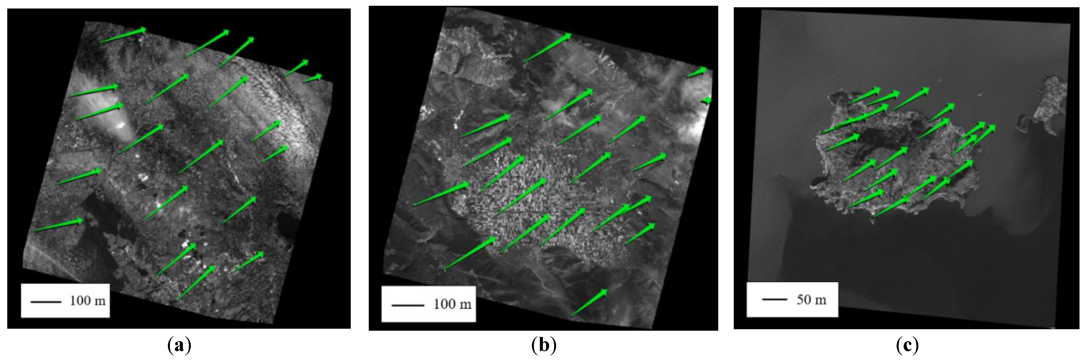
Considering the results obtained, the accuracy achieved by applying the RPC method with bias compensation is acceptable for applications of the hyperspectral data, whose spatial resolution is 30 m per pixel, while it is inappropriate for the correction of panchromatic data, whose spatial resolution is 5 m. Furthermore, the accuracy values obtained in the Ischia test field are decidedly better than in the other two cases. The reason for these different behaviours can be due to the different extension of areas; in fact, the Isle of Ischia occupies only a portion of the whole image with limited extension in latitude and longitude, unlike the other two cases. To further investigate this behavior, a test was carried out in which a 10 km E-W × 8 km N-S portion of the images of the other test-fields was considered (Figure 4).
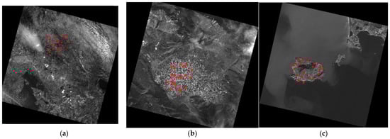
Figure 4.
Ground point distribution for a central area of the image, test field of Rome (a), Fucino (b) and Ischia (c).
The results obtained in the test concentrated in an area of limited extension are reported in Table 8 and Table 9. Similarly to the case of Ischia, acceptable accuracies have already been obtained, starting from the estimation of the RPC order 0 solution with only two GCPs. A further observation is the slight improvement of the accuracy values as the order of the transformation increases. The case study of Rome reached the highest accuracy, especially in the E direction, while the cases of Ischia and Fucino reached an accuracy in the order of 1–2 pixels overall.
Table 8.
Results of RPC bundle adjustment with bias compensation for small-central area of Rome.
Table 9.
Results of RPC bundle adjustment with bias compensation for small-central area of Fucino.
Finally, a small non-central area of the Fucino test field was selected to complete the accuracy analysis as a function of the image extension and GCP distribution (Figure 5). To complete the analysis, four GCPs and four CPs were collimated in the lower right area of test field. The results (Table 10), computed only for RPC order 0 and order 1 solutions, show a clear deterioration in accuracy compared to the solution obtained in the central area of the test field.
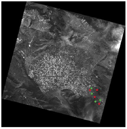
Figure 5.
Ground point distribution for a small area of the image in the lower right corner, test field of Fucino (in red the GCPs, in green the CPs).
Table 10.
Results of RPC bundle adjustment with bias compensation for small area of the image in the lower right corner, test field of Fucino.
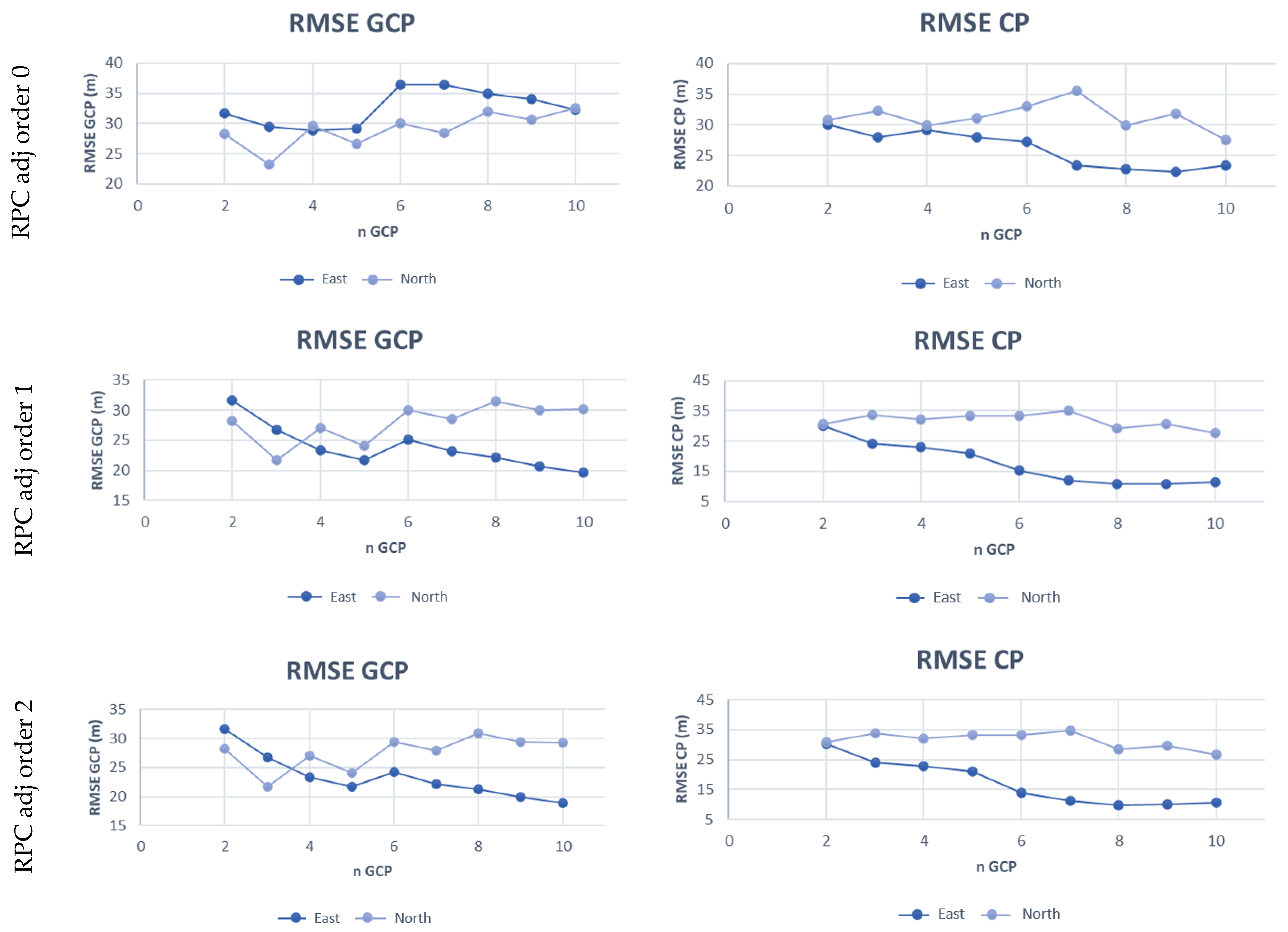
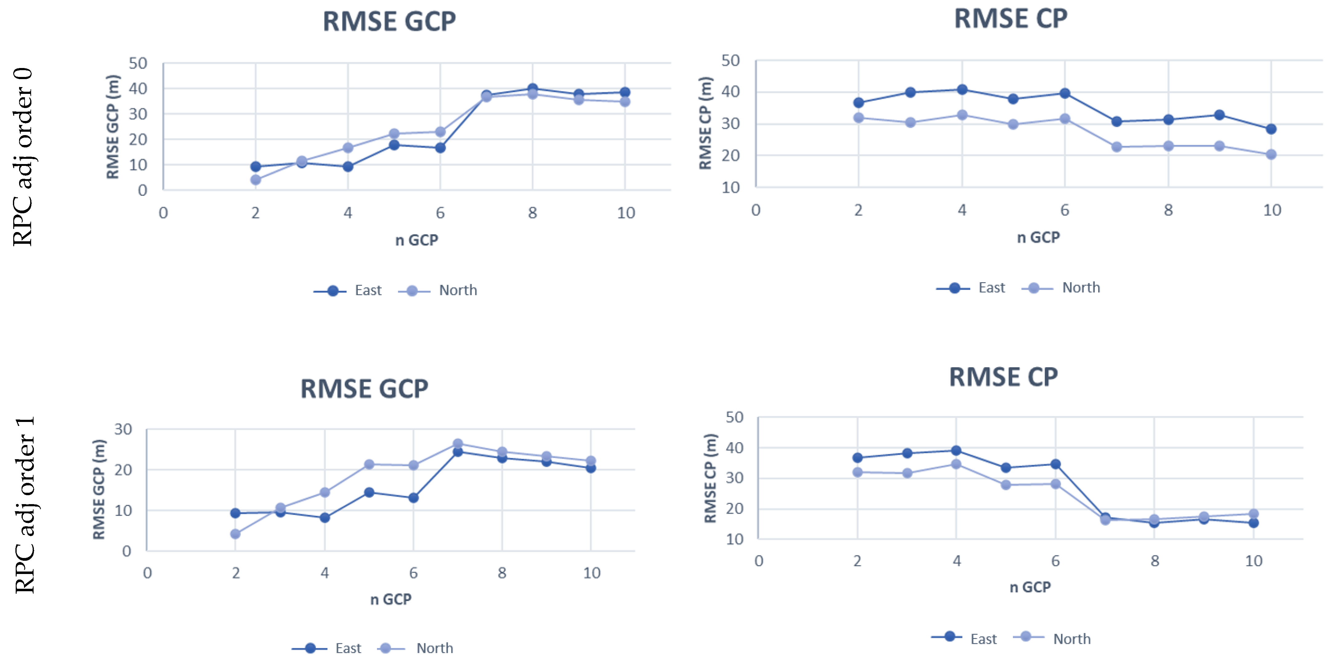
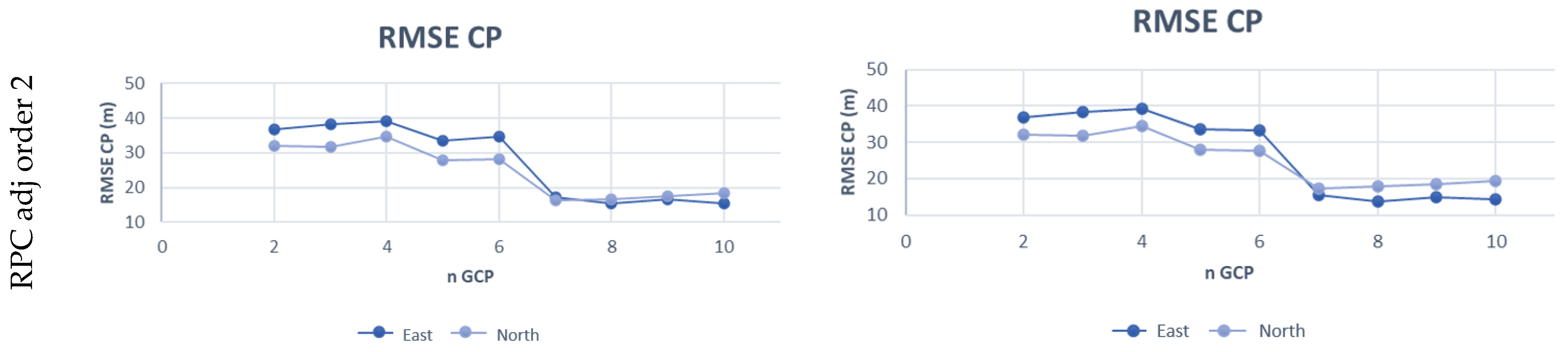
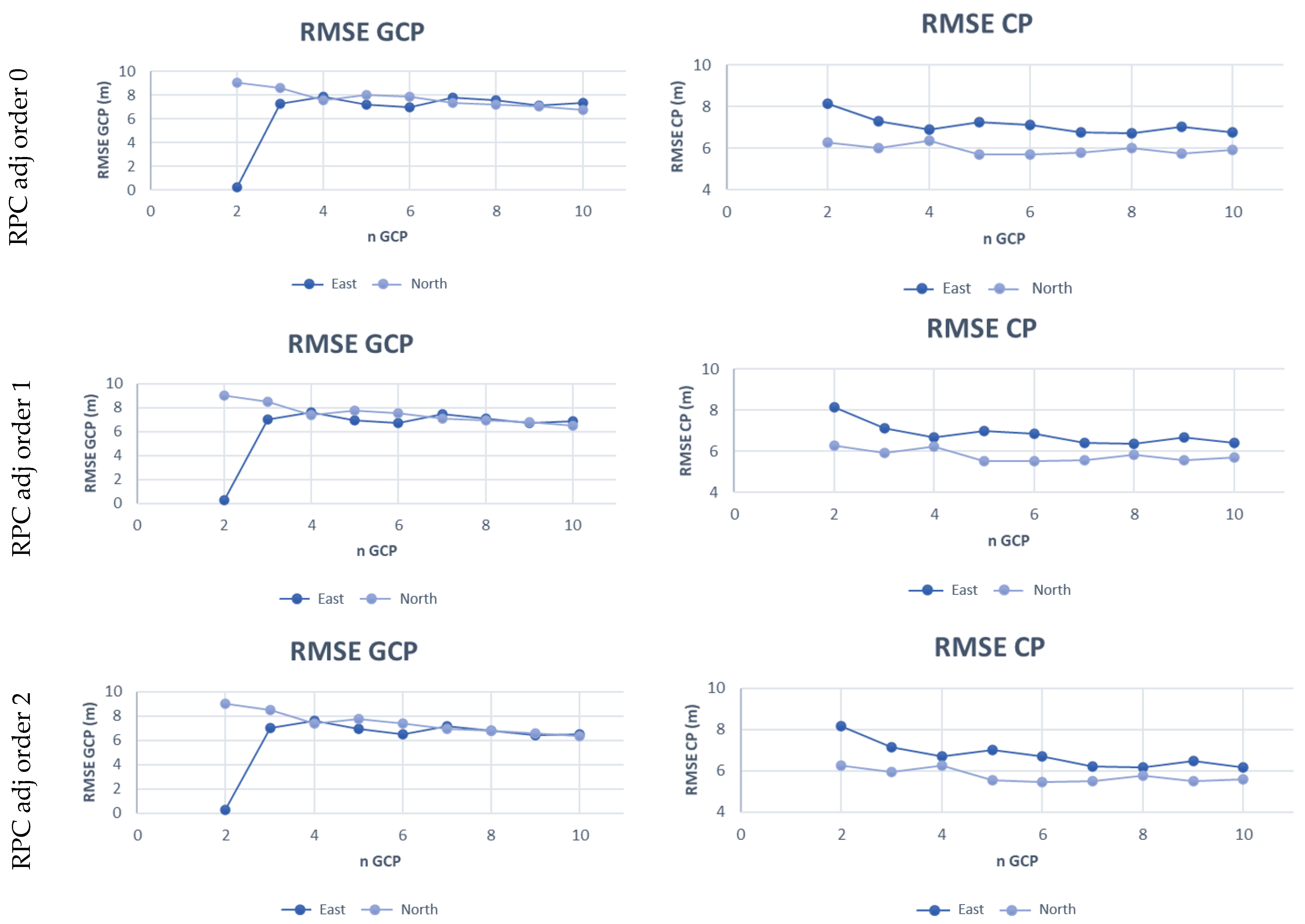
A trend analysis of the results (Figure 6, Figure 7 and Figure 8) was conducted by considering the RMSE of both GCPs and CPs as a function of the GCP number used for orientation model computation. The figures show that both the model precision (RMSE of GCP) and the image accuracy (RMSE of CP) values follow the expected behaviour, that is the former increases while the latter decreases, as the number of GCPs increases. For the test fields of Rome and Fucino, a trend variation between the RPC order 0 and order 1 solutions was observed, while the trends recorded for the test field of Ischia remained unchanged in cases where the order transformation varied, a behavior already noted in the results in Table 5.
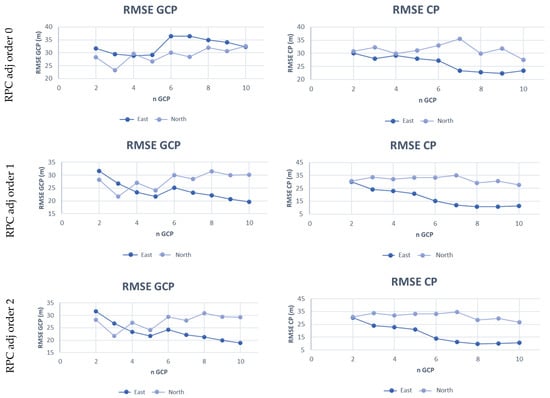
Figure 6.
Precision and accuracy trends for Rome image.
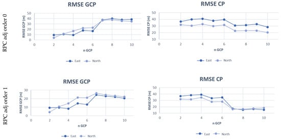
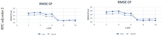
Figure 7.
Precision and accuracy trends for Fucino image.
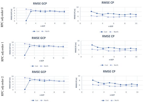
Figure 8.
Precision and accuracy trends for Ischia image.
Considering the results obtained in all tests, the best performance for the orientation with the RCP model of whole images was obtained with RPC order 1 or order 2 transformations, as evidenced by the improvement recorded for the accuracy values in the E direction, while for the orientation with the RCP model of the central area of the image, the RPC order 0 solution with few GCPs reached a constant accuracy.
Moreover, the precision and accuracy trends tend to stabilize as the number of GCPs increases, as is described in the literature [13,22], which in our study started from about 7–8 GCPs. The results shown for the orientations estimated on the basis of a few GCPs, in fact, are affected by the distribution of the GCPs chosen.
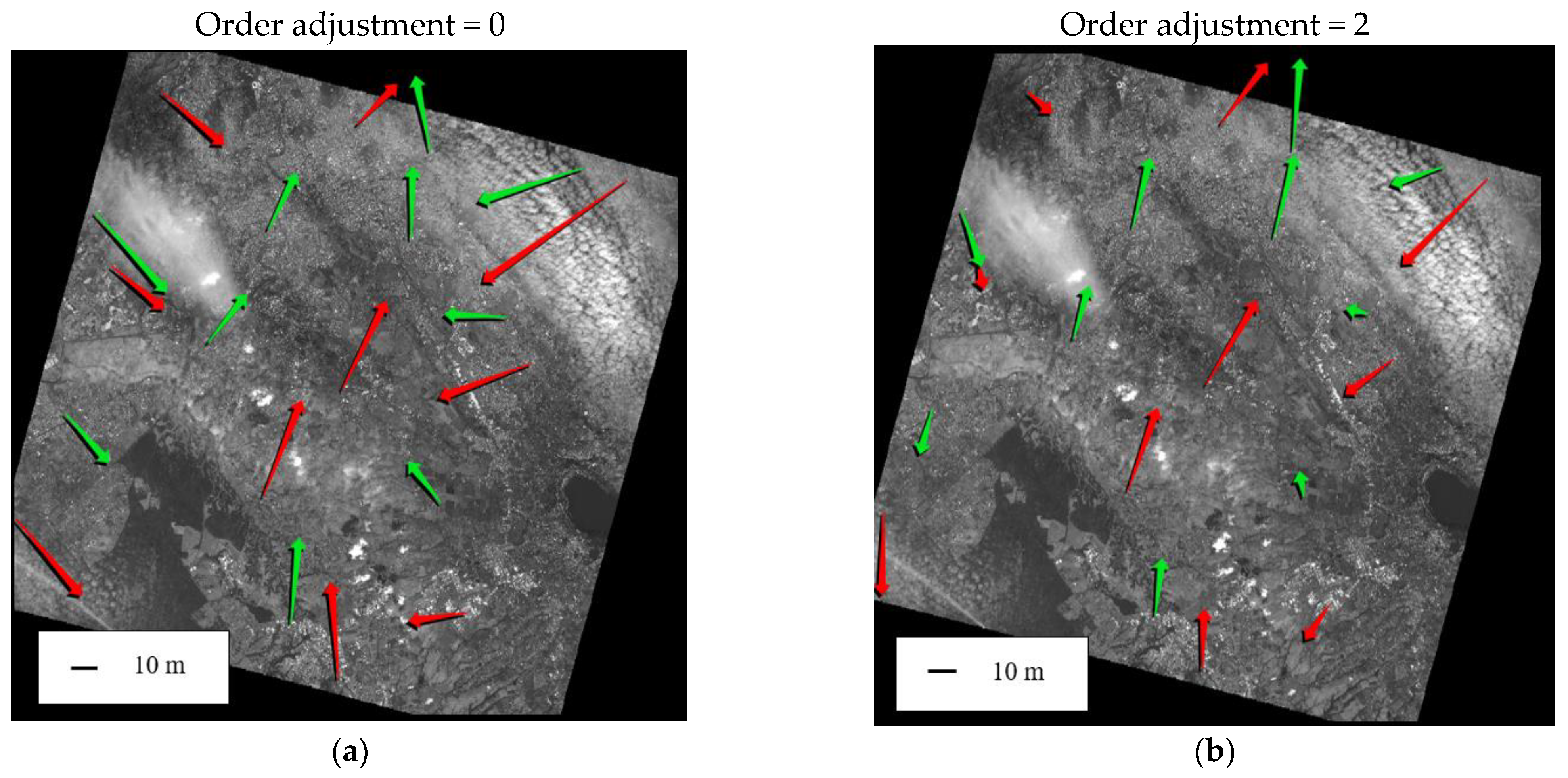
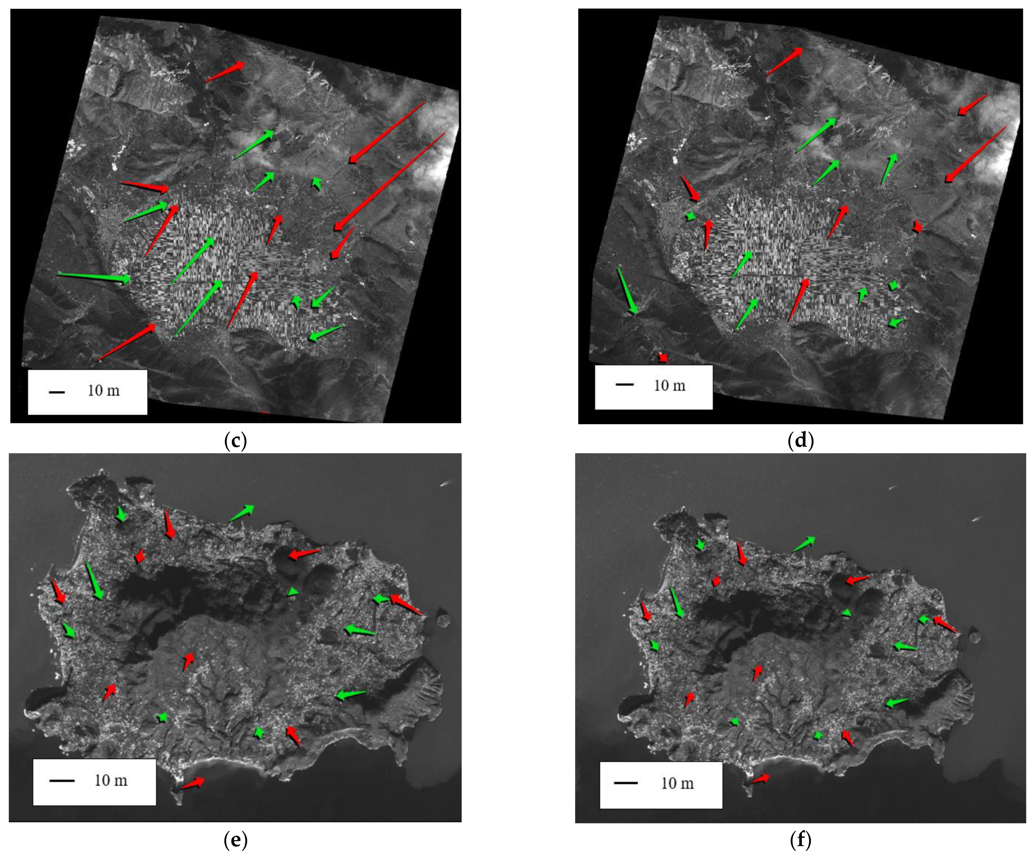
The graphs of the vectors representing the residuals in the E and N directions are shown below. The graphs allow us to highlight the characteristics of the RPC errors; in fact, a random distribution can be interpreted as the absence of the influence of time-dependent drift effects. On the contrary, residuals aligned in the along-track direction show the presence of drift effects and an influence of the scan velocity [15]. A further analysis can be carried out by studying the residuals on individual CPs, and Figure 9 shows the results obtained by applying the RPC model without any refinement. The error is clearly systematic and is partially corrected by RPC order adjustment = 0, which only allows for the estimation of translation parameters (Figure 10a,c,e). Figure 10 shows the residuals of each point (in red the GCPs, in green the CPs) for the different test fields, and for RPC refinement order 0 (Figure 10a,c,e) and order 2 (Figure 10b,d,f). Despite the refinement of RPC parameters, it is still possible to observe a systematic behaviour in the test-fields of Rome and the Fucino plain. The residual vectors of the points distributed on the image perimeter decreased after increasing the order of the transformation, while the errors in the image center remained essentially unchanged. The Isle of Ischia, on the other hand, shows a slight improvement in errors with the RPC bundle adjustment order = 2.
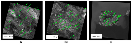
Figure 9.
The planimetric errors—RPC model with no refinements applied, test field of Rome (a), Fucino (b) and Ischia (c).
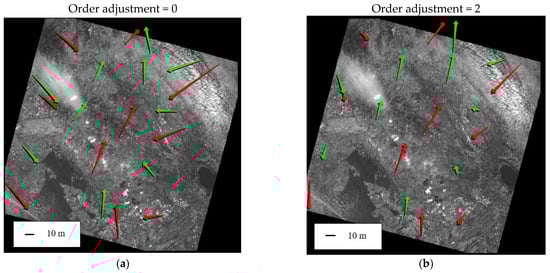
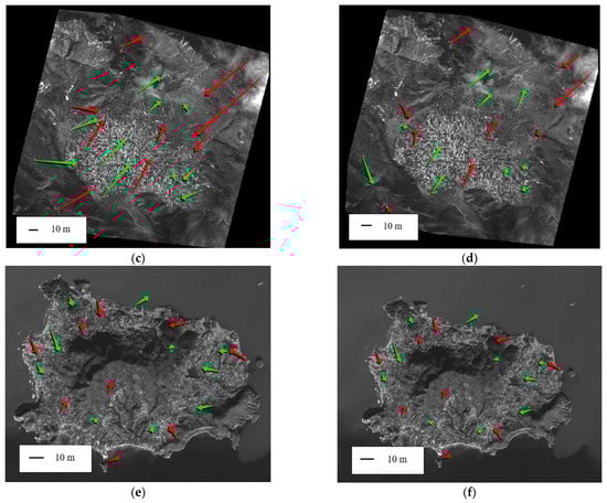
Figure 10.
Planimetric errors for RPC order 0 and order 2 solution—test field of Rome (a,b), Fucino (c,d) and Ischia (e,f).
The results of the accuracies obtained using the RPC models were in agreement with the hypothesis that dividing the image by stripes (E-W direction) or by columns (N-S direction) could improve the results as was the case for highly asynchronous satellites studied previously (e.g., EROS-A); however, these tests did not achieve reliable and unambiguous results and are therefore only reported in Appendix A for completeness.
3.3. RPF Model
3.3.1. Results of RPF Model
The Rational Polynomial Functions without RPCs were analysed to complete the overview of PRISMA performance. In the RPF empirical method, the coefficients were estimated on the basis of a large set of collimated GCPs. The method has been applied on all test fields and a total of 60 points for each image were collimated. Of these, 47 were used as GCPs for coefficients estimation and 13 were used as CPs for validation of the oriented image.
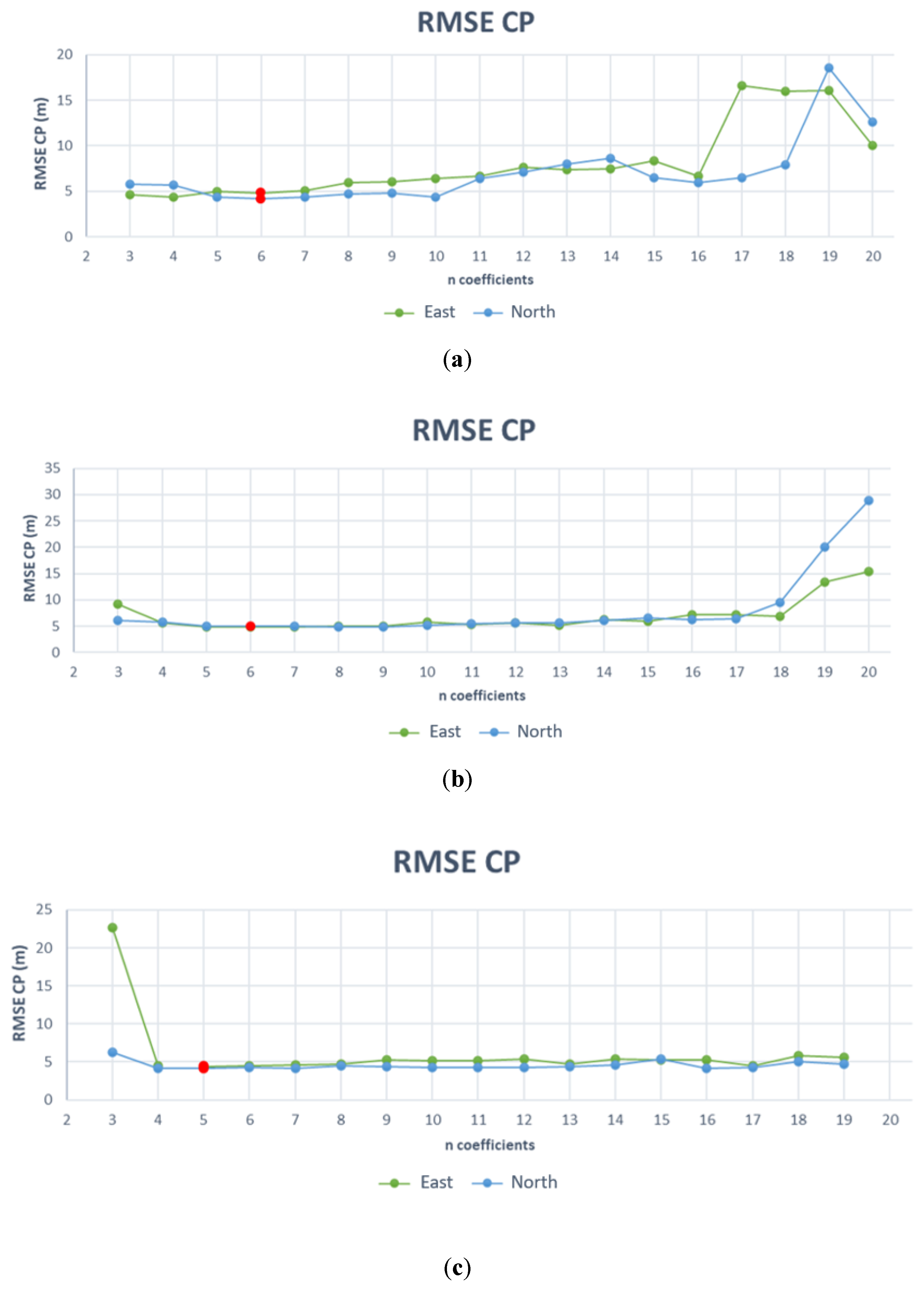
The analysis was performed in OrthoEngine, in which it is possible to set the number of RPF coefficients that need to be estimated. Figure 11 shows the accuracy trend as a function of coefficient numbers, whereby the accuracy decreases as the number of coefficients increases. In particular, the Rome and Fucino test fields show similar behaviour, reaching the best accuracy in the E and N directions when six polynomial coefficients were estimated (Table 11); it should also be noted that the accuracy trends tend to worsen from the estimation of second-degree polynomials function. The results obtained for Ischia show that maximum accuracy was achieved when using five polynomial coefficients (Table 11).
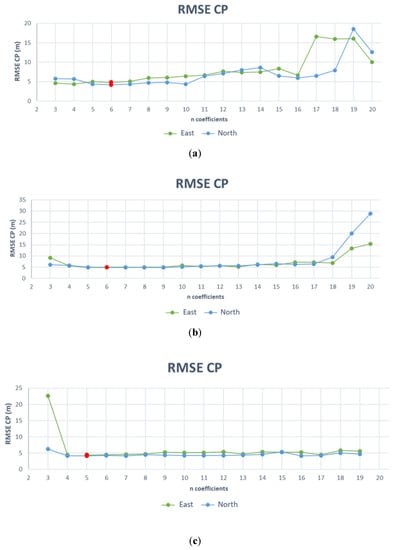
Figure 11.
Accuracy trend as a function of RPC coefficients—test field Rome (a), Fucino (b) and Ischia (c).
Table 11.
Maximum accuracy achieved.
3.3.2. Discussion of RPF Model
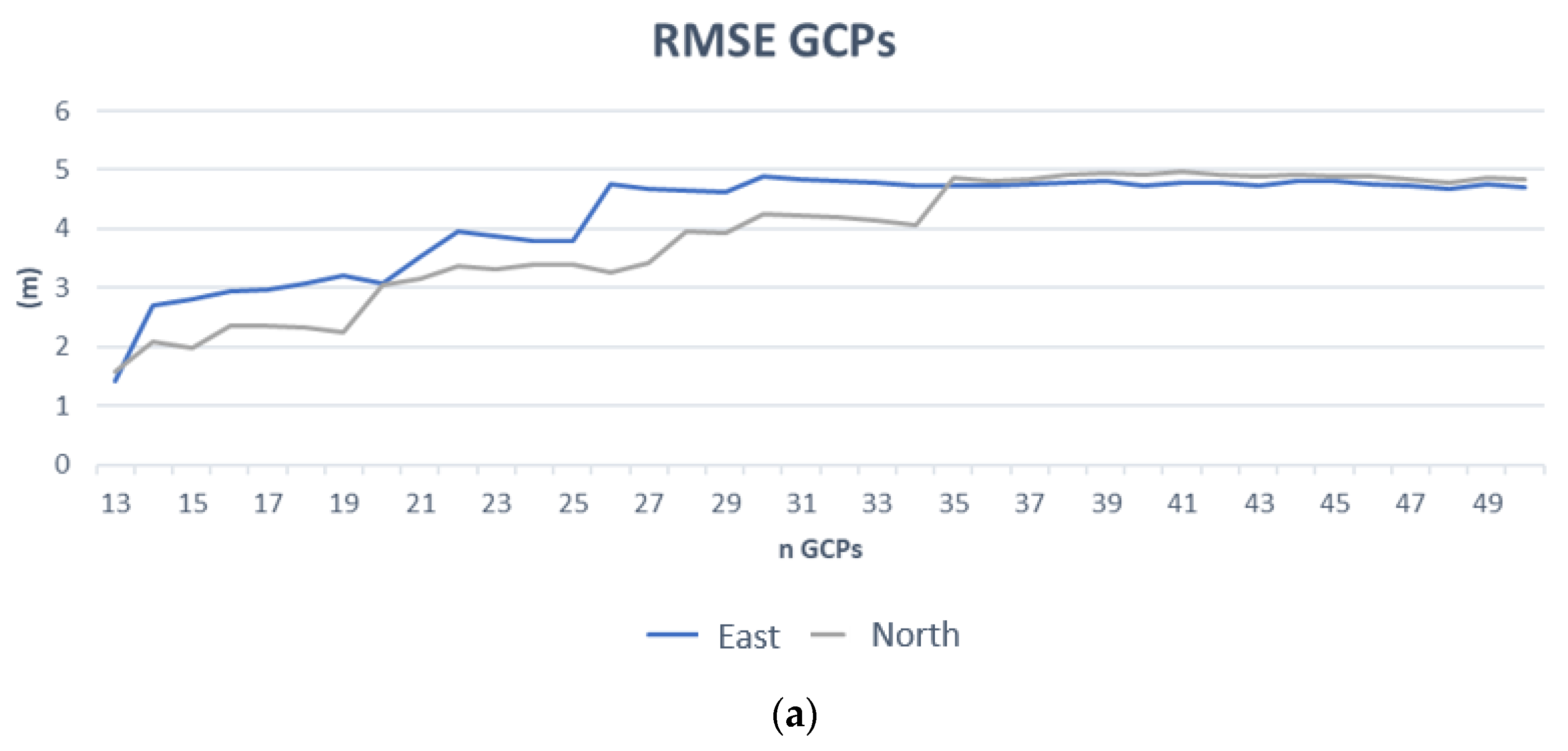
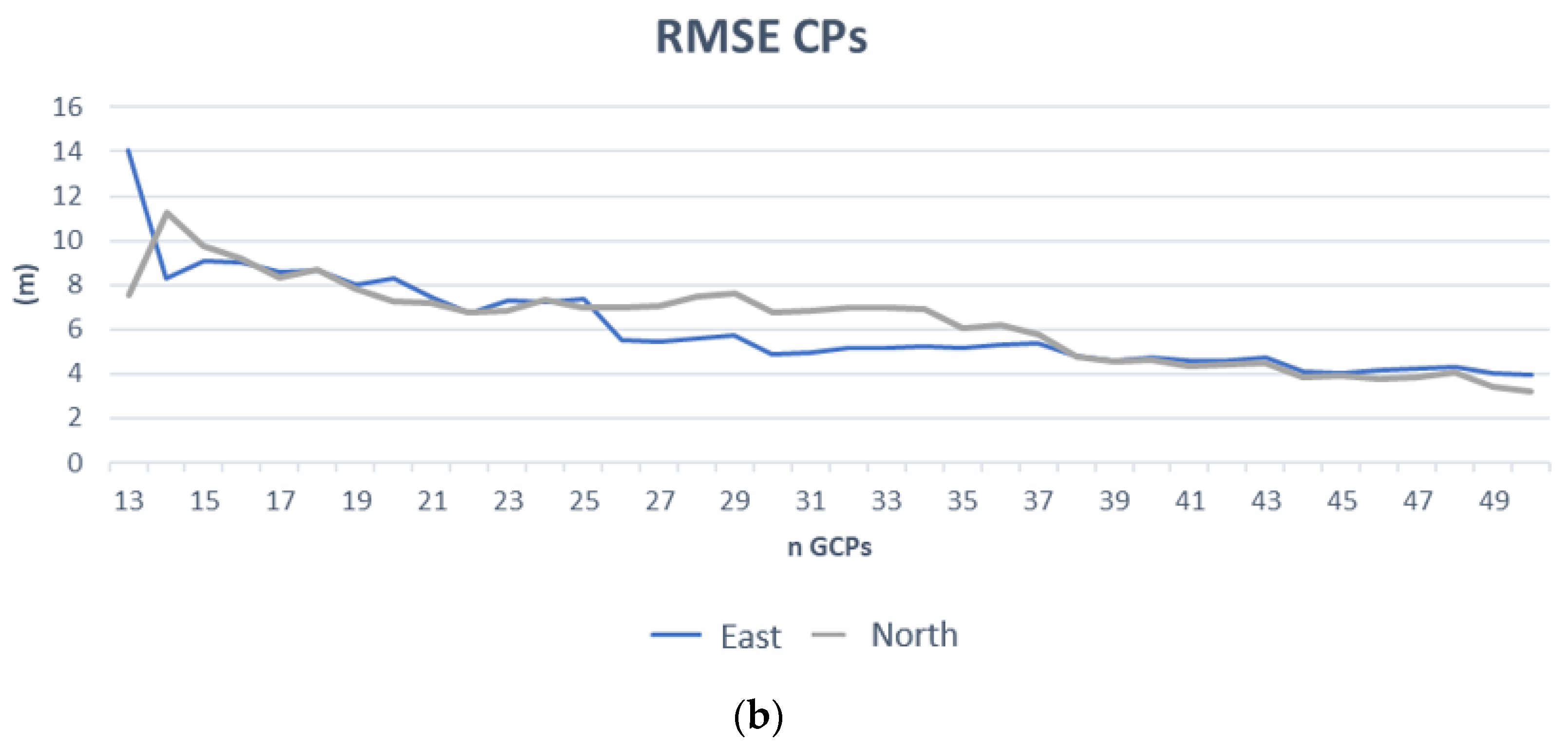
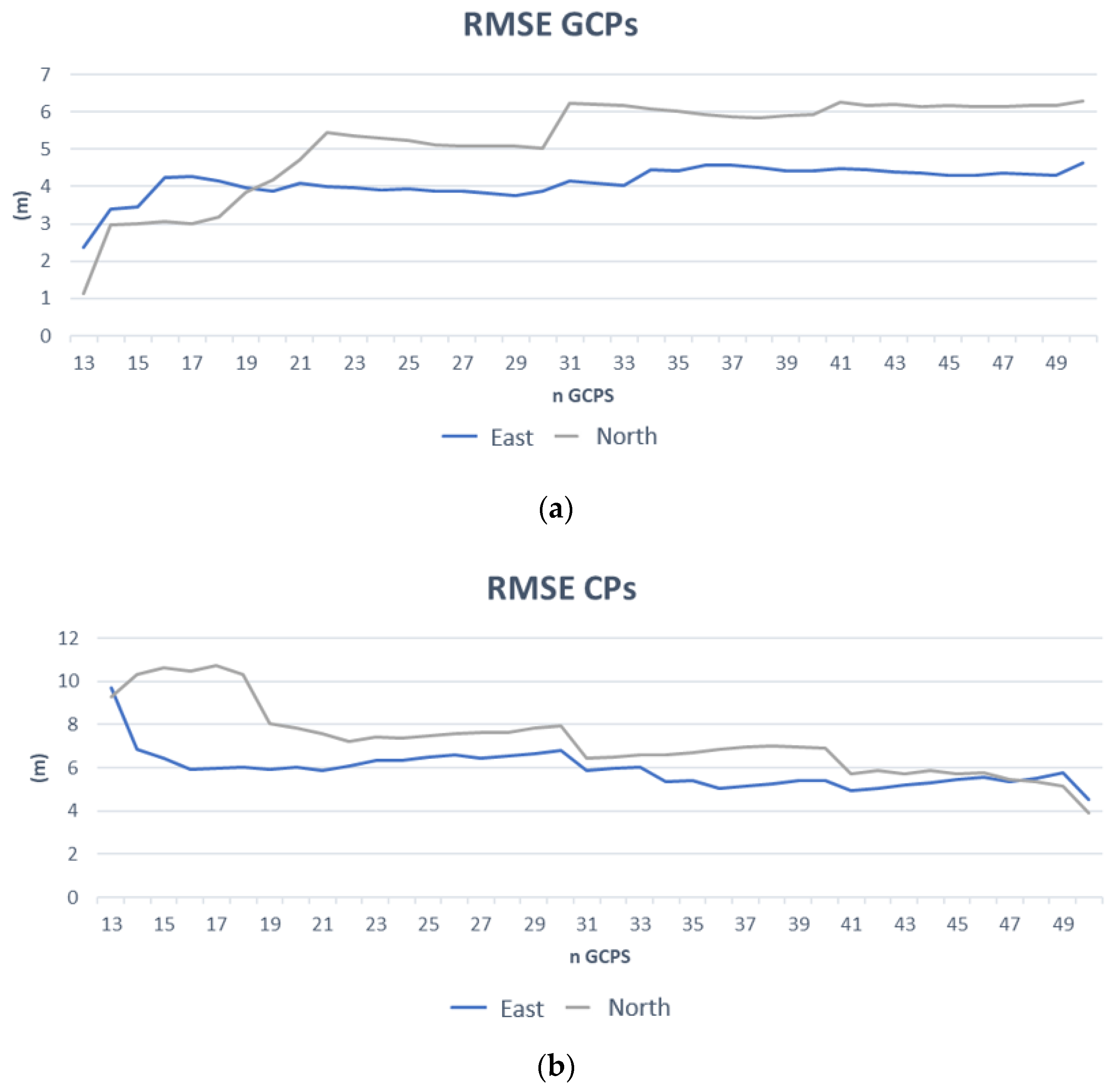
Considering that the most efficient application of RPFs for PRISMA images were reached with six polynomial coefficients, a further investigation was carried out to investigate the necessary number of GCPs to achieve adequate precision and accuracy, considering the resolution of the panchromatic image as a reference (5 m).
The Rome and Fucino images were considered to be representative because the GCPs can be distributed over the entire image, then they were oriented after considering an RPF model with six polynomial coefficients. The model precision (RMSE of GCP, Figure 12a and Figure 13a) and image accuracy (RMSE of CP, Figure 12b and Figure 13b) are analysed as a function of the GCP number.
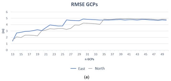
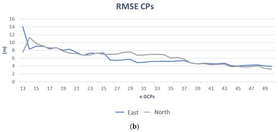
Figure 12.
Trend of precision (a) and accuracy (b) in relation to the number of collimated GCPs, referred to the Rome test field.
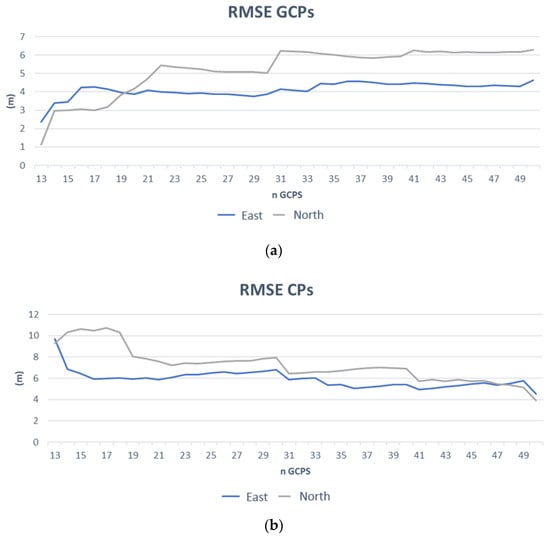
Figure 13.
Trend of precision (a) and accuracy (b) in relation to the number of collimated GCPs, referred to the Fucino test field.
It can be observed that adequate accuracy was reached with 40 GCPs (Table 12) which is certainly a high value of GCPs compared to the 12–20 usually necessary for rigorous models or the 2–4 required for RPCs. Nevertheless, it is important to underline that the panchromatic resolution (5 m) of PRSIMA images does not necessarily require GCPs with decimetre or centimetre precision, so the ground points can be quickly acquired from maps at a scale of 1:10,000 or larger making the process much faster.
Table 12.
Accuracy achieved with 40 GCPs.
4. Conclusions
This study on the possible methods of geometric correction of the PRISMA images provided different results depending on the type of orientation model used.
The tests were carried out on data that had the highest resolution, i.e., the panchromatic image (5 m), while the hyperspectral images were found to have lower resolutions (generally 30 m). The spatial resolution of the images is a fundamental piece of information because the accuracies required to best orthorectify a certain image depend on their specific resolution.
The rigorous model, as we previously estimated, in the OrthoEngine function, has an accuracy of about 20 m with about 12 GCPs over the entire image.
It has to be underlined that, curiously, these results were obtained with an image that was already partly geometrically processed (2d level) while the same model does not converge if we use the raw image, which in theory should provide the best results with this model. This model can be used to orientate, using a small number of points, the hyperspectral layers of the image because it provides accuracies that are compatible with the specific resolutions.
The RPC-based model, whose parameters are declared compliant with the NIMA standard, can achieve accuracies close to the resolution of the panchromatic image (5 m) but only for limited and central areas, as observed in the island example. In such a case, few GCPs are needed to obtain accuracies that are compatible with panchromatic images but, as mentioned, only for limited and centred areas.
Finally, the RPF model seems to achieve the best results; in particular, the six-parameter formulation was the most efficient when using panchromatic PRISMA images. Considering this model, the entire scene can be oriented and consequently orthorectified with an accuracy of around 5 m which is equal to the maximum resolution of the image itself. Since the disadvantage of RPFs with respect to previous models is the high number of GCPs required, the number of GCPs required to provide adequate accuracy was also evaluated. Optimal results seem to be obtained from 40 GCPs; however, GCPs can also be inserted with an accuracy of 2.5 m on the ground, and these accuracies are also easily attainable from high- to medium-scale maps (1:5000–1:10,000) available in many areas, making time-consuming surveying with geodetic class GPS unnecessary. This procedure can therefore be used advantageously on entire scenes even for panchromatic images, as long as a large set of GCPs with metric accuracy is available which can be rapidly obtained, as already mentioned, if cartography (at least at 1:10,000 scale) is available.
For the rigorous model, we are still waiting for the release of some specific functions on commercial software and when they become available, they will be widely tested. In our tests with the rigorous model, the orbital and external orientation parameters used and their sources were specified. These parameters have been included in the OrthoEngine function according to best practices established in the literature. However, the authors are open to suggestions and contributions from the scientific community or platform operators for possible refinements of the model itself.
With regard to the RPC models, the authors expect the possible realization of automatic procedures in commercial software or possible refinements of the RPC sets themselves by the satellite operator.
RPFs, on the other hand, can already be used, even on open-source software, with 40 or more GCPs.
Author Contributions
Conceptualization, V.B., F.G. and F.M.; methodology, V.B., F.G. and F.M.; validation, V.B., F.G. and F.M.; investigation V.B., F.G. and F.M.; writing—original draft preparation, V.B., F.G. and F.M.; writing—review and editing, V.B., F.G. and F.M. All authors have read and agreed to the published version of the manuscript.
Funding
This research was partially funded by Sapienza University, grants number: RP12117A8B237587 and AR12117A8B42362B.
Institutional Review Board Statement
Not applicable.
Informed Consent Statement
Not applicable.
Acknowledgments
The authors would like to thank Marilena Amoroso and Ettore Lopinto of the Italian Space Agency for their useful suggestions and advice; we would also like to thank Luigi Agrimano and Antonio Novelli of Planetek for the useful exchange of information. Finally, we would like to thank the staff of the Metropolitan City of Naples for providing the cartography of the island of Ischia.
Conflicts of Interest
The authors declare no conflict of interest.
Appendix A
The orientation of the panchromatic images of Rome and the Fucino plain shows critical results for the accuracy values in the N direction (Table 6 and Table 7). Considering the pushbroom acquisition mode of the PRISMA satellite, we decided to perform tests by analysing the image of Rome for strips distributed in the North–South and East–West directions (Figure A1). In the case of strips in the North–South direction, a reduced number of image columns was considered, while in the case of East–West strips, a reduced number of image rows was considered. In both cases, a strip extension of approximately 6 km was set and 20 ground points were collimated. Table A1 shows the results obtained by orienting the image with a point distribution in the E-W direction, and the values are similar to those obtained for the whole image. Finally, Table A2 shows the results obtained with a point distribution in the N-S direction; in this case, a substantial improvement of the residuals in the N direction can be seen.
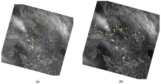
Figure A1.
Ground point distribution in N-S (a) and E-W (b) direction, test field of Rome.
Figure A1.
Ground point distribution in N-S (a) and E-W (b) direction, test field of Rome.

Table A1.
Results of RPC bundle adjustment with bias compensation for strip in E-W direction, Rome test field.
Table A1.
Results of RPC bundle adjustment with bias compensation for strip in E-W direction, Rome test field.
| RPC Bundle Adjustment Solution | N. of GCPs (N. of CP) | RMSE Value of CP Discrepancies. Units Are in Metres | |
|---|---|---|---|
| E | N | ||
| Spatial Intersection | None (20) | 135.128 | 88.883 |
| RPC order 0: X0, Y0 | 2 (18) | 22.968 | 22.47 |
| RPC order 0: X0, Y0 | 7 (13) | 18134 | 23.208 |
| RPC order 1: X0, X1, X2, Y0, Y1, Y2 | 4 (16) | 14.668 | 23.068 |
| RPC order 1: X0, X1, X2, Y0, Y1, Y2 | 7 (13) | 12.96 | 23.177 |
| RPC order 1: X0, X1, X2, Y0, Y1, Y2 | 10 (10) | 9.139 | 22.769 |
| RPC order 2: X0, X1, X2, X3, X4, X5, Y0, Y1, Y2, Y3, Y4, Y5 | 7 (13) | 12.058 | 22.866 |
| RPC order 2: X0, X1, X2, X3, X4, X5, Y0, Y1, Y2, Y3, Y4, Y5 | 10 (10) | 8.106 | 22.467 |
Table A2.
Results of RPC bundle adjustment with bias compensation for strip in N-S direction, Rome test field.
Table A2.
Results of RPC bundle adjustment with bias compensation for strip in N-S direction, Rome test field.
| RPC Bundle Adjustment Solution | N. of GCPs (N. of CP) | RMSE Value of CP Discrepancies. Units Are in Metres | |
|---|---|---|---|
| E | N | ||
| Spatial Intersection | None (20) | 137.997 | 106.319 |
| RPC order 0: X0, Y0 | 2 (18) | 7.842 | 14.759 |
| RPC order 0: X0, Y0 | 7 (13) | 7.881 | 7.355 |
| RPC order 1: X0, X1, X2, Y0, Y1, Y2 | 4 (16) | 7.338 | 7.726 |
| RPC order 1: X0, X1, X2, Y0, Y1, Y2 | 7 (13) | 7.827 | 5.9 |
| RPC order 1: X0, X1, X2, Y0, Y1, Y2 | 10 (10) | 7.63 | 5.98 |
| RPC order 2: X0, X1, X2, X3, X4, X5, Y0, Y1, Y2, Y3, Y4, Y5 | 7 (13) | 7.836 | 5.824 |
| RPC order 2: X0, X1, X2, X3, X4, X5, Y0, Y1, Y2, Y3, Y4, Y5 | 10 (10) | 7.722 | 5.809 |
The best result was obtained by analysing a central area of the image distributed in the N-S direction. For completeness, tests were also repeated for the lateral areas (Figure A2 and Figure A3a,c), to highlight possible dependencies on variable sensor orientation conditions. The behaviors shown by the test fields of Rome and the Fucino plain are very similar; in fact, for the central area, the highest accuracy in both directions E and N, was equal to 1–2 px. On the contrary, the results for the lateral area of the image are worse (Table A3, Table A4, Table A5, Table A6 and Table A7), specifically for the right side that reaches an accuracy of 3–4 px in both directions.
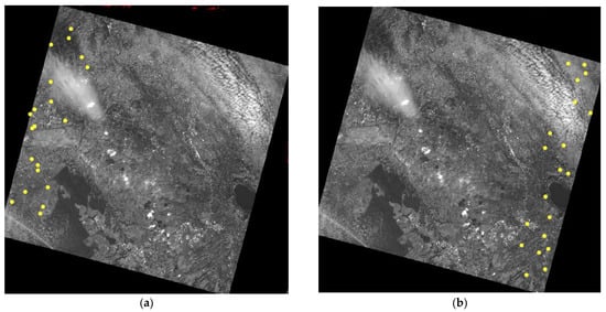
Figure A2.
Ground point distribution in N-S direction in the side areas of the image, Rome test field, west side area in (a) and east side area in (b).
Figure A2.
Ground point distribution in N-S direction in the side areas of the image, Rome test field, west side area in (a) and east side area in (b).
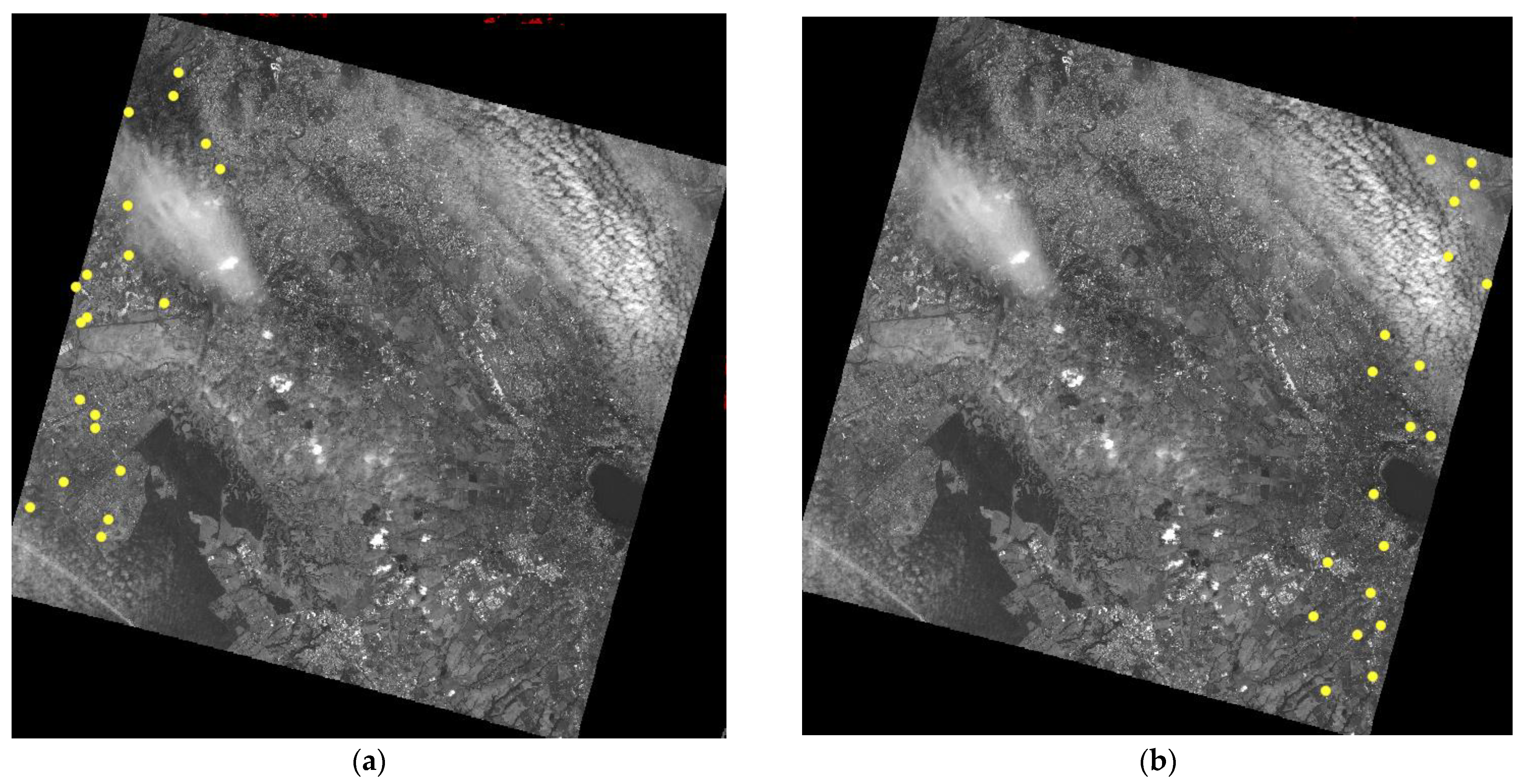
Table A3.
Results of RPC bundle adjustment with bias compensation for strip in N-S direction in the left side, Rome test field.
Table A3.
Results of RPC bundle adjustment with bias compensation for strip in N-S direction in the left side, Rome test field.
| RPC Bundle Adjustment Solution | N. of GCPs (N. of CP) | RMSE Value of CP Discrepancies. Units Are in Metres | |
|---|---|---|---|
| E | N | ||
| Spatial Intersection | None (20) | 156.498 | 57.906 |
| RPC order 0: X0, Y0 | 2 (18) | 5.911 | 21.938 |
| RPC order 0: X0, Y0 | 7 (13) | 5.719 | 19.891 |
| RPC order 1: X0, X1, X2, Y0, Y1, Y2 | 4 (16) | 6.422 | 26.909 |
| RPC order 1: X0, X1, X2, Y0, Y1, Y2 | 7 (13) | 5.601 | 19.708 |
| RPC order 1: X0, X1, X2, Y0, Y1, Y2 | 10 (10) | 6.017 | 20.066 |
| RPC order 2: X0, X1, X2, X3, X4, X5, Y0, Y1, Y2, Y3, Y4, Y5 | 7 (13) | 5.461 | 19.254 |
| RPC order 2: X0, X1, X2, X3, X4, X5, Y0, Y1, Y2, Y3, Y4, Y5 | 10 (10) | 5.854 | 19.507 |
Table A4.
Results of RPC bundle adjustment with bias compensation for strip in N-S direction in the right side, Rome test field.
Table A4.
Results of RPC bundle adjustment with bias compensation for strip in N-S direction in the right side, Rome test field.
| RPC Bundle Adjustment Solution | N. of GCPs (N. of CP) | RMSE Value of CP Discrepancies. Units Are in Metres | |
|---|---|---|---|
| E | N | ||
| Spatial Intersection | None (20) | 61.103 | 30.784 |
| RPC order 0: X0, Y0 | 2 (18) | 22.488 | 21.314 |
| RPC order 0: X0, Y0 | 7 (13) | 17.95 | 18.11 |
| RPC order 1: X0, X1, X2, Y0, Y1, Y2 | 4 (16) | 20.433 | 18.245 |
| RPC order 1: X0, X1, X2, Y0, Y1, Y2 | 7 (13) | 18.934 | 17.415 |
| RPC order 1: X0, X1, X2, Y0, Y1, Y2 | 10 (10) | 17.157 | 17.141 |
| RPC order 2: X0, X1, X2, X3, X4, X5, Y0, Y1, Y2, Y3, Y4, Y5 | 7 (13) | 19.231 | 17.627 |
| RPC order 2: X0, X1, X2, X3, X4, X5, Y0, Y1, Y2, Y3, Y4, Y5 | 10 (10) | 17.212 | 17.099 |
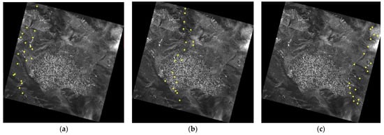
Figure A3.
Ground point distribution in N-S direction in the central (b) and side areas (a) and (c) of the image, Fucino test field.
Figure A3.
Ground point distribution in N-S direction in the central (b) and side areas (a) and (c) of the image, Fucino test field.
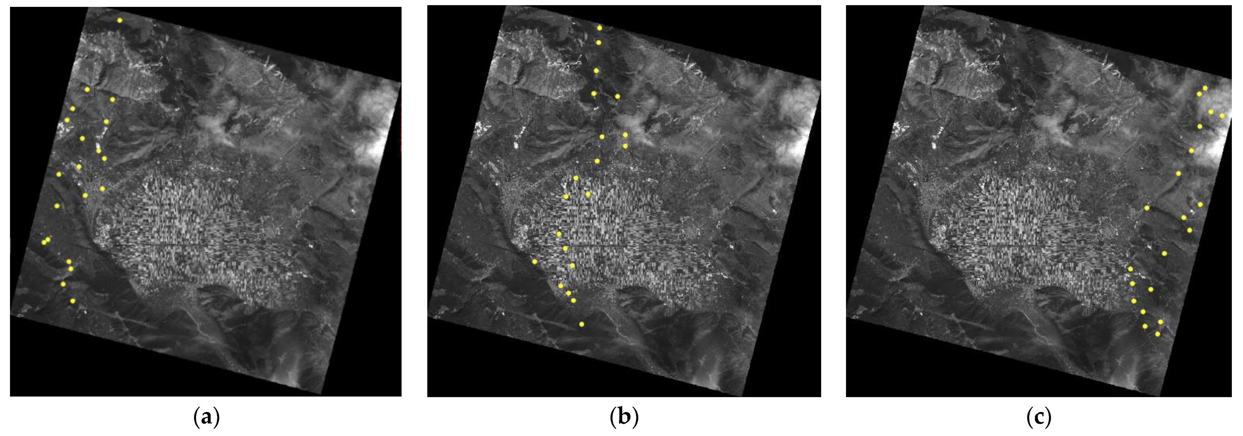
Table A5.
Results of RPC bundle adjustment with bias compensation for central strip in N-S direction, case (b).
Table A5.
Results of RPC bundle adjustment with bias compensation for central strip in N-S direction, case (b).
| RPC Bundle Adjustment Solution | N. of GCPs (N. of CP) | RMSE value of CP Discrepancies. Units Are in Metres | |
|---|---|---|---|
| E | N | ||
| Spatial Intersection | None (20) | 145.989 | 99.858 |
| RPC order 0: X0, Y0 | 2 (18) | 5.439 | 14.128 |
| RPC order 0: X0, Y0 | 7 (13) | 5.478 | 15.798 |
| RPC order 1: X0, X1, X2, Y0, Y1, Y2 | 4 (16) | 5.359 | 11.891 |
| RPC order 1: X0, X1, X2, Y0, Y1, Y2 | 7 (13) | 5.365 | 12.217 |
| RPC order 1: X0, X1, X2, Y0, Y1, Y2 | 10 (10) | 4.759 | 11.402 |
| RPC order 2: X0, X1, X2, X3, X4, X5, Y0, Y1, Y2, Y3, Y4, Y5 | 7 (13) | 5.317 | 11.414 |
| RPC order 2: X0, X1, X2, X3, X4, X5, Y0, Y1, Y2, Y3, Y4, Y5 | 10 (10) | 4.833 | 10.582 |
Table A6.
Results of RPC bundle adjustment with bias compensation for left strip in N-S direction, case (a).
Table A6.
Results of RPC bundle adjustment with bias compensation for left strip in N-S direction, case (a).
| RPC Bundle Adjustment Solution | N. of GCPs (N. of CP) | RMSE Value of CP Discrepancies. Units Are in Metres | |
|---|---|---|---|
| E | N | ||
| Spatial Intersection | None (20) | 158.24 | 71.255 |
| RPC order 0: X0, Y0 | 2 (18) | 11.925 | 24.684 |
| RPC order 0: X0, Y0 | 7 (13) | 9.409 | 26.421 |
| RPC order 1: X0, X1, X2, Y0, Y1, Y2 | 4 (16) | 11.043 | 22.122 |
| RPC order 1: X0, X1, X2, Y0, Y1, Y2 | 7 (13) | 8.672 | 24.179 |
| RPC order 1: X0, X1, X2, Y0, Y1, Y2 | 10 (10) | 8.37 | 21.756 |
| RPC order 2: X0, X1, X2, X3, X4, X5, Y0, Y1, Y2, Y3, Y4, Y5 | 7 (13) | 8.818 | 23.152 |
| RPC order 2: X0, X1, X2, X3, X4, X5, Y0, Y1, Y2, Y3, Y4, Y5 | 10 (10) | 8.667 | 20.454 |
Table A7.
Results of RPC bundle adjustment with bias compensation for right strip in N-S direction, case (c).
Table A7.
Results of RPC bundle adjustment with bias compensation for right strip in N-S direction, case (c).
| RPC Bundle Adjustment Solution | N. of GCPs (N. of CP) | RMSE Value of CP Discrepancies. Units Are in Metres | |
|---|---|---|---|
| E | N | ||
| Spatial Intersection | None (20) | 66.662 | 32.143 |
| RPC order 0: X0, Y0 | 2 (18) | 21.436 | 29.653 |
| RPC order 0: X0, Y0 | 7 (13) | 18.004 | 17.514 |
| RPC order 1: X0, X1, X2, Y0, Y1, Y2 | 4 (16) | 17.631 | 20.029 |
| RPC order 1: X0, X1, X2, Y0, Y1, Y2 | 7 (13) | 17.41 | 16.395 |
| RPC order 1: X0, X1, X2, Y0, Y1, Y2 | 10 (10) | 17.071 | 15.243 |
| RPC order 2: X0, X1, X2, X3, X4, X5, Y0, Y1, Y2, Y3, Y4, Y5 | 7 (13) | 17.369 | 16.287 |
| RPC order 2: X0, X1, X2, X3, X4, X5, Y0, Y1, Y2, Y3, Y4, Y5 | 10 (10) | 17.022 | 15.102 |
References
- Koçal, A.; Duzgun, H.S.; Karpuz, C. Discontinuity Mapping with Automatic Lineament Extraction from High Resolution Satellite Imagery; ISPRS XX: Istanbul, Turkey, 2004; pp. 12–23. [Google Scholar]
- Chen, T.; Trinder, J.C.; Niu, R. Object-Oriented Landslide Mapping Using ZY-3 Satellite Imagery, Random Forest and Mathematical Morphology, for the Three-Gorges Reservoir, China. Remote Sens. 2017, 9, 333. [Google Scholar] [CrossRef] [Green Version]
- Lu, H.; Ma, L.; Fu, X.; Liu, C.; Wang, Z.; Tang, M.; Li, N. Landslides Information Extraction Using Object-Oriented Image Analysis Paradigm Based on Deep Learning and Transfer Learning. Remote Sens. 2020, 12, 752. [Google Scholar] [CrossRef] [Green Version]
- Rostami, M.; Kolouri, S.; Eaton, E.; Kim, K. Deep Transfer Learning for Few-Shot SAR Image Classification. Remote Sens. 2019, 11, 1374. [Google Scholar] [CrossRef] [Green Version]
- Baiocchi, V.; Brigante, R.; Dominici, D.; Milone, M.V.; Mormile, M.; Radicioni, F. Automatic three-dimensional features extraction: The case study of L’Aquila for collapse identification after April 06, 2009 earthquake. Eur. J. Remote Sens. 2014, 47, 413–435. [Google Scholar] [CrossRef]
- Transon, J.; D’Andrimont, R.; Maugnard, A.; Defourny, P. Survey of Hyperspectral Earth Observation Applications from Space in the Sentinel-2 Context. Remote Sens. 2018, 10, 157. [Google Scholar] [CrossRef] [Green Version]
- Pignatti, S.; Acito, N.; Amato, U.; Casa, R.; Bonis, R.d.; Diani, M.; Laneve, G.; Matteoli, S.; Palombo, A.; Pascucci, S.; et al. Development of algorithms and products for supporting the Italian hyperspectral PRISMA mission: The SAP4PRISMA project. In Proceedings of the 2012 IEEE International Geoscience and Remote Sensing Symposium, Munich, Germany, 22–27 July 2012; pp. 127–130. [Google Scholar]
- Guarini, R.; Loizzo, R.; Facchinetti, C.; Longo, F.; Ponticelli, B.; Faraci, M.; Dami, M.; Cosi, M.; Amoruso, L.; de Pasquale, V.; et al. Prisma Hyperspectral Mission Products. In Proceedings of the IEEE International Geoscience and Remote Sensing Symposium, IGARSS ’18, Valencia, Spain, 22–27 July 2018; pp. 179–182. [Google Scholar]
- Loizzo, R.; Daraio, M.; Guarini, R.; Longo, F.; Lorusso, R.; Dini, L.; Lopinto, E. Prisma Mission Status and Perspective. In Proceedings of the IEEE International Geoscience and Remote Sensing Symposium, IGARSS ’19, Yokohama, Japan, 28 July–2 August 2019; pp. 4503–4506. [Google Scholar]
- Giardino, C.; Bresciani, M.; Braga, F.; Fabbretto, A.; Ghirardi, N.; Pepe, M.; Gianinetto, M.; Colombo, R.; Cogliati, S.; Ghebrehiwot, S.; et al. First Evaluation of PRISMA Level 1 Data for Water Applications. Sensors 2020, 20, 4553. [Google Scholar] [CrossRef] [PubMed]
- Vangi, E.; D’Amico, G.; Francini, S.; Giannetti, F.; Lasserre, B.; Marchetti, M.; Chirici, G. The New Hyperspectral Satellite PRISMA: Imagery for Forest Types Discrimination. Sensors 2021, 21, 1182. [Google Scholar] [CrossRef] [PubMed]
- Busetto, L.; Ranghetti, L. Prismaread: A Tool for Facilitating Access and Analysis of PRISMA L1/L2 Hyperspectral Imagery v1.0.0. 2020. Available online: https://lbusett.github.io/prismaread/ (accessed on 22 February 2022).
- Toutin, T. Review article: Geometric processing of remote sensing images: Models, algorithms and methods. Int. J. Remote Sens. 2004, 25, 1893–1924. [Google Scholar] [CrossRef]
- Poli, D. A Rigorous Model for Spaceborne Linear Array Sensors. Photogramm. Eng. Remote Sens. 2007, 73, 187–196. [Google Scholar] [CrossRef] [Green Version]
- Mikhail, E.M.; Bethel, J.S.; McGlone, J.C. Introduction to Modern Photogrammetry; Wiley: Hoboken, NJ, USA, 2001; ISBN 978-0-471-30924-6. [Google Scholar]
- Fraser, C.S.; Hanley, H.B. Bias-compensated RPCs for Sensor Orientation of High-resolution Satellite Imagery. Photogramm. Eng. Remote Sens. 2005, 71, 909–915. [Google Scholar] [CrossRef]
- Tong, X.; Liu, S.; Weng, Q. Bias-corrected rational polynomial coefficients for high accuracy geo-positioning of QuickBird stereo imagery. ISPRS J. Photogramm. Remote Sens. 2010, 65, 218–226. [Google Scholar] [CrossRef]
- Meguro, Y.; Fraser, C.S. Georeferencing accuracy of Geoeye-1 stereo imagery: Experiences in a Japanese test field. Int. Arch. Photogramm. Remote Sens. Spat. Inf. Sci. 2010, 38, 1069–1072. [Google Scholar]
- Poli, D.; Toutin, T. Review of developments in geometric modelling for high resolution satellite pushbroom sensors. Photogramm. Rec. 2012, 27, 58–73. [Google Scholar] [CrossRef]
- Rupnik, E.; Deseilligny, M.P.; Delorme, A.; Klinger, Y. Refined satellite image orientation in the free open-source photogrammetric tools apero/micmac. ISPRS Ann. Photogramm. Remote Sens. Spat. Inf. Sci. 2016, III-1, 83–90. [Google Scholar] [CrossRef] [Green Version]
- Hanley, H.B.; Fraser, C.S. Sensor orientation for high-resolution satellite imagery: Further insights into bias-compensated RPCs. Photogramm. Eng. Remote Sens. 2004, 71. Available online: https://www.researchgate.net/publication/228806391_Sensor_orientation_for_high-resolution_satellite_imagery_Further_insights_into_bias-compensated_RPCs (accessed on 22 February 2022).
- Jacobsen, K. Systematic geometric image errors of very high resolution optical satellites. ISPRS Int. Arch. Photogramm. Remote Sens. Spat. Inf. Sci. 2018, XLII-1, 233–238. [Google Scholar] [CrossRef] [Green Version]
- Zhou, G.; Li, R. Accuracy Evaluation of Ground Points from IKONOS High-Resolution Satellite imagery. Photogramm. Eng. Remote. Sens. 2000, 66, 1103–1112. [Google Scholar]
- Baiocchi, V.; Giannone, F.; Monti, F.; Vatore, F. ACYOTB plugin: Tool for accurate orthorectification in open-source environments. ISPRS Int. J. Geo Inf. 2019, 9, 11. [Google Scholar] [CrossRef] [Green Version]
- Poli, D.; Remondino, F.; Angiuli, E.; Agugiaro, G. Radiometric and geometric evaluation of GeoEye-1, WorldView-2 and Pléiades-1A stereo images for 3D information extraction. ISPRS J. Photogramm. Remote Sens. 2015, 100, 35–47. [Google Scholar] [CrossRef]
- Agugiaro, G.; Poli, D.; Remondino, F. Testfield Trento: Geometric Evaluation Of Very High Resolution Satellite Imagery. ISPRS Int. Arch. Photogramm. Remote Sens. Spat. Inf. Sci. 2012, XXXIX-B1, 191–196. [Google Scholar] [CrossRef] [Green Version]
- Zheng, X.; Huang, Q.; Wang, J.; Wang, T.; Zhang, G. Geometric Accuracy Evaluation of High-Resolution Satellite Images Based on Xianning Test Field. Sensors 2018, 18, 2121. [Google Scholar] [CrossRef] [PubMed] [Green Version]
- Tarquini, S.; Isola, I.; Favalli, M.; Battistini, A. TINITALY, a Digital Elevation Model of Italy with a 10 Meters Cell Size (Version 1.0) [Data Set]; Istituto Nazionale di Geofisica e Vulcanologia (INGV): Rome, Italy, 2007. [CrossRef]
- National Imagery and Mapping Agency. “The Compendium of Controlled Extensions (CE) for the National Imagery Transmission Format (NITF)”, VERSION 2.1, 16 November 2000. Available online: http://geotiff.maptools.org/STDI-0002_v2.1.pdf (accessed on 22 February 2022).
- Loizzo, R.; Ananasso, C.; Guarini, R.; Lopinto, E.; Candela, L.; Pisani, A.R. The prisma hyperspectral mission. In Proceedings of the Living Planet Symposium, Prague, Czech Republic, 9–13 May 2016; pp. 9–13. [Google Scholar]
- PRISMA: La Missione Iperspettrale Nazionale, Conferenza 2018. Available online: http://conferenzecisam.it/convegni/c-i-s-a-m-2018-1/documenti/Loizzo_PRISMA%20La%20missione%20iperspettrale%20nazionale.pdf (accessed on 22 February 2022).
- IFAC CNR, Progetto Optima. 2014. Available online: http://www.ifac.cnr.it/corsari/meteors/private/OPTIMA%20-%20PRISMA%20Products%20and%20Applications%20-%20140930.pdf (accessed on 22 February 2022).
- Guarini, R.; Loizzo, R.; Longo, F.; Mari, S.; Scopa, T.; Varacalli, G. Overview of the PRISMA space and ground segment and its hyperspectral products. In Proceedings of the IEEE International Geoscience and Remote Sensing Symposium (IGARSS), Fort Worth, TX, USA, 23–28 July 2017; pp. 431–434. [Google Scholar] [CrossRef]


Publisher’s Note: MDPI stays neutral with regard to jurisdictional claims in published maps and institutional affiliations. |
© 2022 by the authors. Licensee MDPI, Basel, Switzerland. This article is an open access article distributed under the terms and conditions of the Creative Commons Attribution (CC BY) license (https://creativecommons.org/licenses/by/4.0/).