Abstract
Shallow estuarine habitats are globally undergoing rapid changes due to climate change and anthropogenic influences, resulting in spatiotemporal shifts in distribution and habitat extent. Yet, scientists and managers do not always have rapidly available data to track habitat changes in real-time. In this study, we apply a novel and a state-of-the-art image segmentation machine learning technique (DeepLab) to two years of high-resolution drone-based imagery of a marine flowering plant species (eelgrass, a temperate seagrass). We apply the model to eelgrass (Zostera marina) meadows in the Morro Bay estuary, California, an estuary that has undergone large eelgrass declines and the subsequent recovery of seagrass meadows in the last decade. The model accurately classified eelgrass across a range of conditions and sizes from meadow-scale to small-scale patches that are less than a meter in size. The model recall, precision, and F1 scores were 0.954, 0.723, and 0.809, respectively, when using human-annotated training data and random assessment points. All our accuracy values were comparable to or demonstrated greater accuracy than other models for similar seagrass systems. This study demonstrates the potential for advanced image segmentation machine learning methods to accurately support the active monitoring and analysis of seagrass dynamics from drone-based images, a framework likely applicable to similar marine ecosystems globally, and one that can provide quantitative and accurate data for long-term management strategies that seek to protect these vital ecosystems.
Keywords:
shallow estuarine habitat; eelgrass; drones; machine learning; coastal dynamics; climate; Morro Bay 1. Introduction
Marine habitats are threatened globally [1] and there is a need to monitor changes and determine appropriate management actions at increasingly rapid timescales [2,3]. One critical marine ecotone is the estuary habitat. Estuaries are critical interfaces between freshwater and marine environments. Although among the world’s most productive ecosystems, estuaries are under an increasing threat from the confluence of climate change, urban development, and pollution [4]. Moreover, estuaries are particularly responsive to environmental changes because estuary species are living near the edges of their tolerances [5,6]. Thus, estuaries may serve as sensitive indicators of global climate change [7].
Seagrass ecosystems are one of the most important habitats in estuaries, while also being some of the most threatened habitats, with documented global declines since the early 1900s [8,9,10,11]. Eelgrass (Zostera marina, a seagrass species of temperate waters) is a habitat-forming marine angiosperm native to nearshore ecosystems across global temperate systems [8]. They provide ecological services, including pathogen remediation [12], carbon sequestration, ocean acidification amelioration, and sediment stabilization, while supporting species with cultural, economic (e.g., global commercial harvested species) and ecological importance [2,4,13,14,15,16,17]. Habitat change can occur due to either large-scale environmental or physical ecosystem changes [18] or due to small-scale environmental variability [19]. There is a growing need to monitor and assess estuarine seagrass dynamics over time to better understand their role in altering marine ecosystem health and resilience.
Several papers have described small-scale estuary and eelgrass spatial habitat dynamics on the Pacific Coast, including archival studies and field investigations [20,21], coastal shoreline surveys [22], and satellite-based methods [23]. Satellite-based methods are also sensitive to image-degrading atmospheric effects and weather (e.g., fog and cloud cover in coastal environments), although they can be a low-cost method for large-scale substrate mapping [21,22,23]. Alternatively, unmanned aircraft systems (UAS; hereafter, drones) can provide high-resolution photographs and geospatial data for wildlife surveys [24,25], the identification of individual flora or fauna [26], and photogrammetry [27]. Drone-based data acquisition for ecological applications has increased rapidly [28] and thus so has the need to rapidly analyze existing imagery to facilitate proactive management.
Drone-based imagery can be collected directly by individual researchers with millimeter to centimeter scale spatial resolution [29,30]. Furthermore, the timing of surveys and spatial coverage can be tailored for specific questions, unlike satellite-based products, allowing for efficient and on-demand sampling. This flexibility is critical for detecting small-scale environmental change and identifying causal processes. Drones have now been used to assess wave run-up on shorelines [31], ocean temperature [23], ocean aerosols [32], algae biomass [33], and coastal geomorphology [34], and sensors have been developed for the high-resolution mapping of parameters such as sea surface salinity [35], the health of coral reefs [36] and seagrass beds [37], shoreline habitat mapping and coastal erosion studies [34], and in assessing the health and abundance of marine vertebrates [38,39]. Drones can detect individual seagrass patches on the order of millimeter to centimeter scale spatial resolution, while typical remote sensing products are limited to more meadow-scale on the order of tens to hundreds of meters.
The availability of small, low-cost, easy-to-fly consumer drones has the potential to transform how natural resource managers work to assess and conserve seagrass and shallow marine habitats, but only if there are quick and accurate habitat classification algorithms and training datasets that are widely available. Currently, and historically in most cases, the data collected from drone sampling regimes are assessed manually. This typically requires extensive hours of manual labor by trained scientists scanning photos and identifying organisms and may sometimes result in observer bias in counts [28]. To address this analytical bottleneck, machine learning techniques have increasingly been paired with drone imagery over the last decade to assess geospatial imagery and habitat extent and are growing in popularity for habitat classification [40,41,42,43,44,45,46,47]. Machine learning methods allow for the rapid identification and documentation of estuary spatial habitat dynamics and can support increasing data robustness and data-driven management actions to conserve and protect these critical habitats.
There are a broad range of studies that have applied machine learning techniques to coastal, estuary, and other marine habitats, including ensemble methods, random forest machine learning algorithms, support vector machine algorithms, and object-based image classification techniques [44,48,49,50,51,52]. However, for drone data specifically, prior research has typically focused on statistical methods such as Z-score normalizations, maximum likelihood classifiers [53] or random forest classifiers [54]. Given the high-resolution imagery captured from drones, image segmentation techniques may prove more accurate compared to traditional image classification techniques since they provide exact outlines of objects in a scene at the level of pixel-by-pixel resolution. Here, we apply an image segmentation technique (DeepLab), previously applied in terrestrial ecosystems [55], to assess dynamics of change in eelgrass habitat.
Although previous work has studied automatic or semi-automatic segmentation and classification of eelgrass (Z. marina) from drone-based data [16,17,18,32], this study is the first to our knowledge to evaluate the application of deep learning methods for this task. This is also the first study to our knowledge to evaluate automatic eelgrass delineation in the California Current at a high-resolution scale on the order of cm. We study eelgrass spatial habitat dynamics in the Morro Bay Estuary of California, an estuary that has undergone large declines and the subsequent recovery of eelgrass over the past decade [17,33,34]. Furthermore, this work is unique in that we evaluate the potential of longitudinal analysis for the study of eelgrass spatial dynamics by training the classifier on data from one year and evaluating its ability to identify eelgrass in data from the next year.
2. Materials and Methods
2.1. Site Description
Morro Bay is a relatively small (~930 hectares) semi-enclosed shallow estuarine ecosystem, located south of Monterey Bay and north of Point Conception State Marine Reserve, along an underexamined stretch of the California coast [56]. Morro Bay not only supports a wide variety of bird, fish, mammalian, and invertebrate communities [57], but is also a popular tourist destination, home to a fishing port for local fisheries [47], and supports two commercial shellfish aquaculture operations. The Morro Bay estuary is approximately 3 km wide and 8 km long and has a main channel that is lined by large expanses of intertidal flats, once dominated by the major biogenic habitat of eelgrasses. The spatial distribution of eelgrass beds throughout Morro Bay has declined since 2007, from 139.2 ha in 2007 to less than 6 ha in 2017, although there are signs of a recovery in recent years [17]. Historically, multispectral imagery obtained from aerial flyovers was used to map eelgrass habitat distributions in Morro Bay; however, since this method is cost-prohibitive, surveys were only conducted intermittently, and as a result, major periods of transition and change were sometimes missed (see, e.g., [17]).
2.2. Data Collection
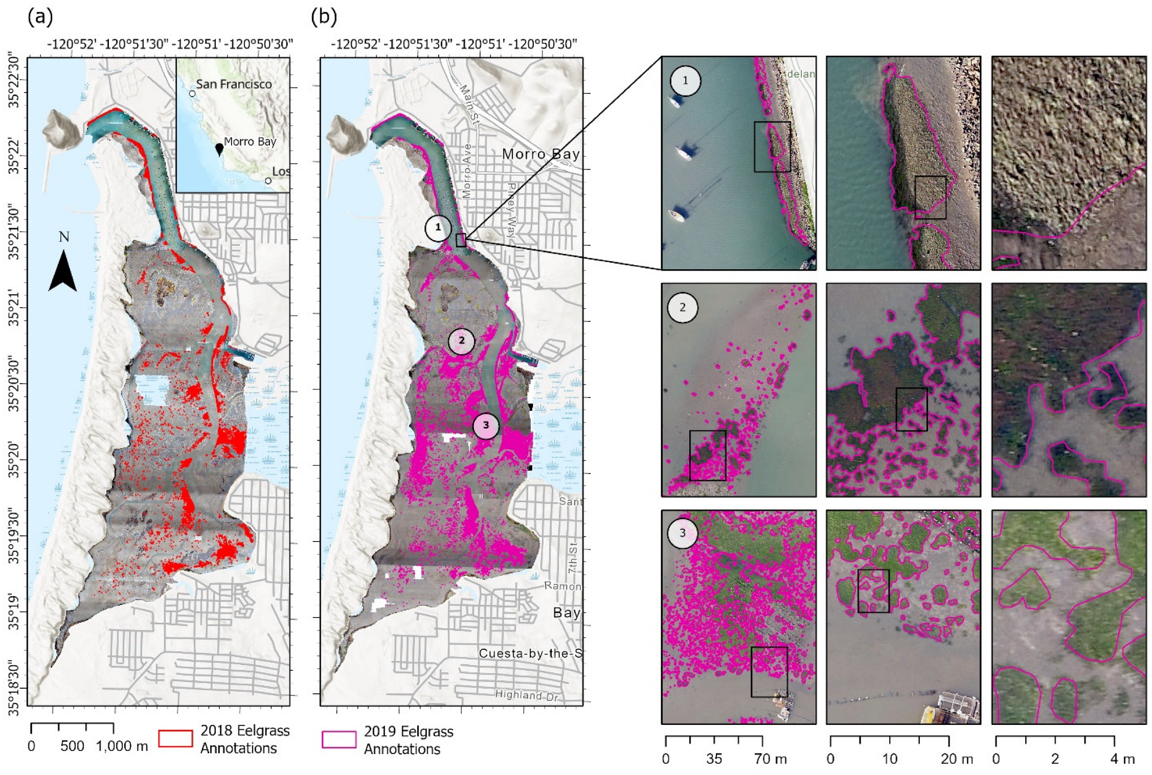
Eelgrass coverage in Morro Bay was mapped using a DJI Phantom 4 Pro drone equipped with a high-resolution camera (20 mp). The drone was flown in November and December of both 2018 and 2019, during 4–5 non-consecutive days of extreme low tides (with flight times of roughly 1 h per day due to low tide limitations) when the intertidal flats and eelgrass beds were exposed, typically at tides lower than approximately −0.3 m relative to the mean lower low water (MLLW). We used the first year of data in 2018 to train the machine learning model and applied it to the second year of data in 2019 to test the model accuracy (Figure 1).
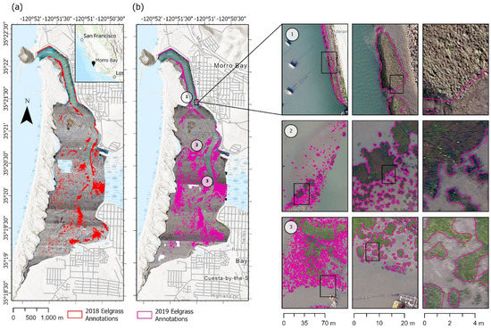
Figure 1.
(Left) Human-annotated images of Morro Bay eelgrass habitats from (a) 2018 and (b) 2019. (Right) The three rows on the right highlight three regions of the estuary in 2019 at varying levels of zoom, as indicated by each inset. (1) Dense bed toward the mouth of estuary that is above water, appearing a light gray-green color; (2) partially submerged beds of varying size mid-estuary that are darker green and have some red-brown coloration and gleam off blades of eelgrass; (3) smaller, younger beds that are not submerged and appear lighter green in the images.
The drone was flown at low altitude (122 m), which results in fine-resolution imagery (~3.35 cm/pixel), providing the ability to resolve fine-scale features and individual eelgrass patches. Following the generation of georectified (map-based registration of an image), estuary-wide orthomosaics (~5000 images per year), the manual classification of the eelgrass habitat during both years of data was performed by a team of geographic information systems (GIS) specialists. This included varying levels of iterative validation checks, including the ground-truthing of areas that had multiple species or limiting weather factors (e.g., low light). A grid was used to ensure all areas of the bay were considered. The threshold for the smallest bed size to digitize was set at a 0.9 m length scale based on image resolution. Each GIS specialist manually digitized polygons, delineating each patch of eelgrass they could identify, and all images were spot-checked by another person. For each year, this digitization process took about 1000 h. The total eelgrass acreage was 6.6 ha and 14.9 ha in 2018 and 2019, respectively [17].
2.3. Machine Learning Model
2.3.1. Image Segmentation
We used an object-oriented machine learning approach called semantic image segmentation (semantic segmentation hereafter). Semantic segmentation is an image-based machine learning neural network technique that delineates objects within an image. The input to a semantic segmentation model is the raster dataset. The output of a semantic segmentation model is a segmentation map of the input image, where each pixel value (one for each band within a pixel, with values ranging from 0 to 255) is transformed into a class label value (that is, 0, 1, 2, …, n). The machine learning algorithm behind semantic segmentation is a convolutional neural network, an algorithm that allows the model to learn the patterns and distinct characteristics of the labeled objects within a given dataset [58]. In this study, we built a binary image segmentation model, where each pixel belonged to one of two classes: an eelgrass or a non-eelgrass class.
2.3.2. Training Data Preparation
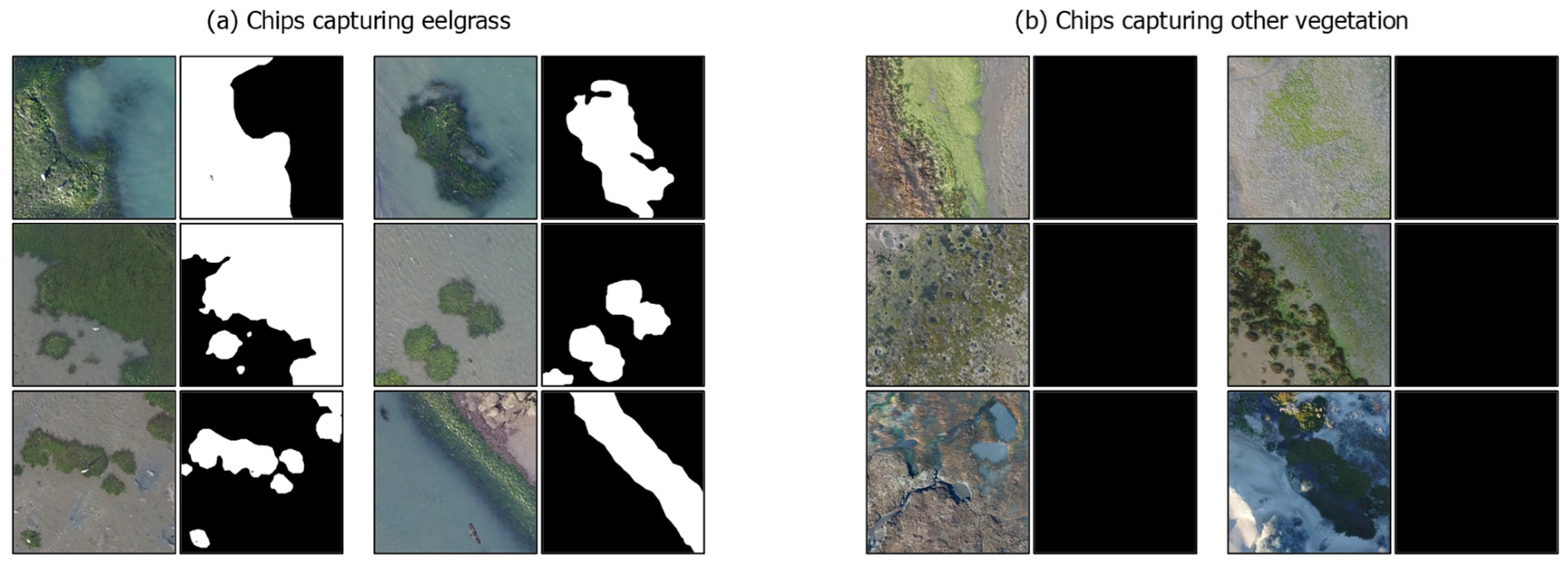
We used the 2018 raster dataset for model training and the 2019 raster dataset for model testing. We exported the data from the human-annotated eelgrass polygons of the 2018 raster dataset. We set the chip size to 448 × 448 pixels and the stride value at 224 pixels, which is equivalent to a 50% overlap between consecutive chips. With these settings, each exported training chip contained a 448 × 448 input image clipped from the 2018 raster dataset and a segmentation image that denoted the class value of each pixel of the input image (e.g., eelgrass or non-eelgrass) (Figure 2a).

Figure 2.
Example training chips for the machine learning pipeline. Each training chip is a pair of images where the left one is the input clipped from the 2018 raster dataset, and the right one is a segmentation image for the input. (a) Chips capturing eelgrass are annotated with white pixels for eelgrass class and black pixels for non-eelgrass class; (b) chips capturing other vegetation contain no eelgrass class, annotated with all black pixels for non-eelgrass class.
Most of the training chips contained annotations of the eelgrass within the image, hence, we added extra chips that had no annotations. To eliminate potential false positives, we exported training chips containing other vegetation classes that were visually similar to eelgrass (e.g., macroalgae such as Ulva spp. and Gracilaria spp.). Each of these training chips was assigned with a non-eelgrass class value (Figure 2b).
2.3.3. Model Training
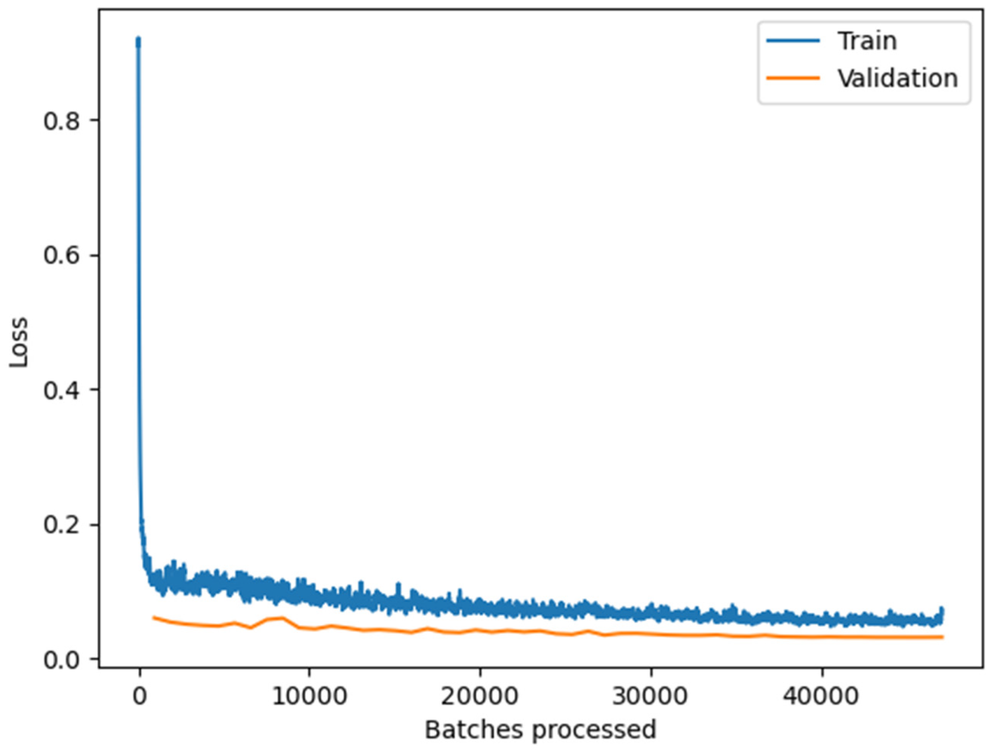
We trained a DeepLab v3 model [59] using the ArcGIS Learn Python module. We evaluated model performance on two well-known backbone architectures for image classification, Resnet 50 and Resnet 101, classes of deep neural networks applied to analyzing visual imagery [60]. We found that the Resnet 50 backbone architecture provided faster training and inference times with comparable accuracy to Resnet 101. As a result, we used Resnet 50 as the backbone architecture for the final model. We used a validation split of 20 percent of the training data, and we did not observe overfitting (Figure 3 and Figure 4).
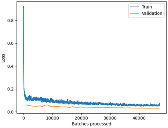
Figure 3.
The training and validation loss graph of the DeepLab V3 model (Resnet 50). After processing the 200,000 training patches, training and validation losses are stabilized at the minimum, indicating that the model does not overfit the training dataset.
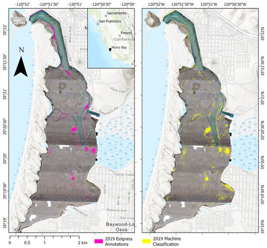
Figure 4.
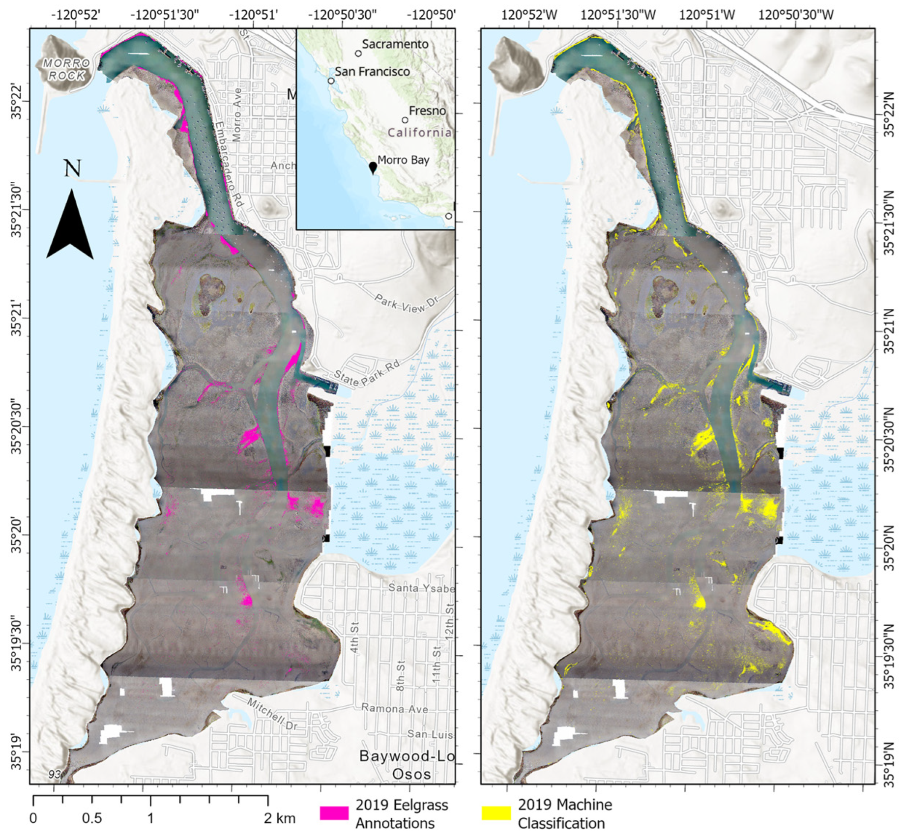
Qualitative comparison of the model eelgrass classification versus human annotation on the entire study area.
With a batch size of 20, we trained the model on 50 epochs and saved the best model obtained during training. We used ArcGIS’s Learn built-in function to determine the optimal learning rate to train the model. ArcGIS Learn utilizes FastAI’s learning rate finding algorithm [61]. The optimal learning rate (the step size in gradient descent) found by this algorithm with the Adam optimizer was 3.6 × 10⁻³ at the beginning, decaying linearly after each epoch to 3.6 × 10⁻⁴ when training was completed. Initially, we utilized a higher learning rate so that the model would learn patterns in the training data more rapidly. As the model approached the optimum learning point, where the lowest loss value in the validation set occurred, we used a lower learning rate. This ensured that the model oscillated around this optimum point, so as to not move farther away from the optimum point during the refinement process [62].
2.3.4. Model Testing
The DeepLab model was evaluated on the 2019 raster dataset and inference was run to obtain a class map. Over 1 million accuracy assessment points were randomly generated throughout the domain for the purpose of comparing class values from the map against the human-annotated and ground-truthed polygon shapefile for each point. The results of these comparisons were used to compute a confusion matrix for model performance evaluation. We also computed the harmonic mean between precision and recall obtaining an F1 score, a performance metric that ranges between 0 and 1 for model performance [63].
3. Results
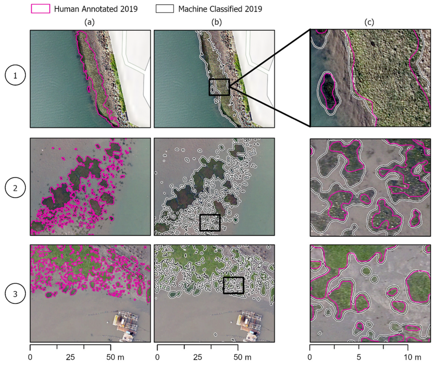
The model was able to accurately identify and annotate eelgrass throughout the estuary, recognizing variability in color, texture, and shape/size (Figure 5). In several places, it was more precise than human annotators. The model more closely traced the outline of beds without cutting off edges based on later visual inspection of images. This was true for multiple eelgrass patches, including larger beds (Figure 1 and Figure 5a) and smaller patchy ones (Figure 2b and Figure 5a).

Figure 5.
Model success cases. Human eelgrass annotations compared to machine-annotated classifications in the three areas of the estuary shown in Figure 1. Column (a,b) show the same area of the estuary with human and model annotations, respectively, while column (c) shows the two annotations overlapped and zoomed in to see differences in annotations more clearly. (1) The machine annotation can capture larger beds and accurately capture the perimeter on par with human annotations. (2) Smaller, patchy beds that the machine annotations more precisely outline beds than the human annotations. (3) The model can pick up on smaller beds that are missed or deemed too small to annotate in human annotations.
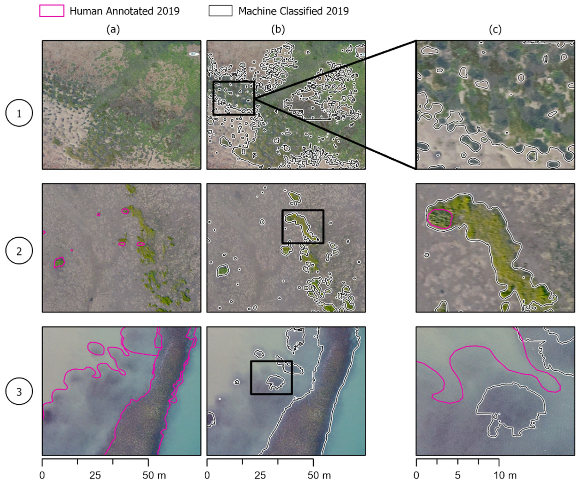
For the accuracy assessment points, there were many true positives (7286) and a low number of false negatives (334). The recall value was relatively high at 0.954. Our qualitative assessment demonstrated that often, false positives were the result of the model classifying mixed macroalgae or terrestrial vegetation as eelgrass. The remaining false positives were the result of shadowed water being classified as eelgrass. The false negatives, which represented 344 ground truth points, were primarily in regions where eelgrass beds were partially submerged, and human annotators assumed continuous beds (Figure 6b). There were a few larger patches and thousands of smaller patches of eelgrass which were detected by the model, but completely missed by human annotators. For the assessment points, there was a moderate number of false positives (3088) that resulted in a lower precision value of 0.723. Thus, among the total pixels that the model classified as eelgrass, approximately 72.3 percent of them were truly eelgrass. The F1 score for the model data was 0.809.
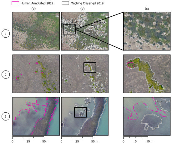
Figure 6.
Similar to Figure 5, but with regard to model failure cases. (1) False positives: A bed of mixed macroalgae that the model annotates as eelgrass. (2) False positives: A bed primarily made up of Ulva spp., with some eelgrass that the model annotates as being entirely eelgrass. (3) False negatives: a partially submerged bed that was inferred to be all eelgrass by annotator. The model annotated the parts of the bed that are less submerged.
To verify the effectiveness of our model, we compared the performance of our DeepLab model to a baseline (Table 1). Our baseline model was U-Net [64], an older deep learning semantic segmentation model with simpler structures and fewer parameters. Our DeepLab model has a slightly lower precision (0.723 versus 0.803), a higher recall (0.954 versus 0.652) and higher F1 score (0.809 versus 0.720). With a higher F1 score overall, our model is more effective at segmenting eelgrass patches.

Table 1.
Confusion matrix for Resnet50 DeepLab v3 model on the 2019 raster dataset.
4. Discussion
Understanding, monitoring, and modeling small-scale marine habitat dynamics require accurate and high-resolution spatial information. In this study, we applied a supervised and a state-of-the-art deep learning model for semantic image segmentation to estuary-wide drone imagery and demonstrated high accuracy for the classification of eelgrass patches relative to human-annotated images. This combined drone-machine learning method has potential to improve the time, cost, and resolution of previous field- and aerial flyover-based methods in Morro Bay. We demonstrate high accuracy for the classification of eelgrass relative to human-annotated images. The model recall, precision, and F1 scores were 0.954, 0.723, and 0.809, respectively, when using human-annotated training data and random assessment points, and our results were either comparable to or demonstrated greater accuracy than other models for similar systems [65,66].
In the existing literature on the drone-based mapping of seagrass habitats, other pixel-based machine learning techniques achieved anywhere between 51 percent to 82 percent model F1 score accuracies [67,68,69,70,71,72,73,74]. Studies with more than 90 percent accuracy usually combined two or more machine learning techniques [75], used a combination of statistics and machine learning techniques [49], or used underwater imagery or ROV data to gather even more fine-resolution data of eelgrass patches and sometimes individual eelgrass blades [76].
A limitation in these types of studies on marine estuaries is the variation in seagrass patch extent, density, bed size, color, and lighting in the imagery. Capturing all the variation that would be seen between different years of drone flights is difficult with a single year of training data and will be the subject of future work. A larger concern is the amount of another habitat present (e.g., macroalgae). In this system, macroalgae (Ulva spp., Chaetomorpha, and Gracilaria) can appear similar in the drone imagery, and often coexist with eelgrass. Often, the macroalgae will mix with eelgrass or grow in layers on top of beds of eelgrass. This results in more discrepancies in training data, as it is difficult to set a threshold for how much of a bed must be eelgrass to be classified as so, and whether a bed that is covered in, for example Ulva spp., should be annotated or left out. It also decreases the performance of the machine learning model, as shown by the large source of false positives from macroalgae (Figure 6). To improve the model accuracy, a multi-class image classification model with a class label for each type of vegetation could be developed. This would require additional training data for each vegetation class and is the subject of future work. Furthermore, the vertical range of the intertidal habitat requires extended periods of low tides where most of the eelgrass is exposed during daylight hours (~4–5 h of tides below −0.3 m MLLW in this site). This time constraint, which will vary depending on the vertical range of the intertidal target species, may limit the applicability of drone-based methods in much larger systems and more regional analyses, at least with current technologies. In these situations, a hybrid method that utilizes satellite-based products for coarser-scale patterns and drone-based products for finer-scaler patterns, or where higher accuracy is needed, may prove effective and is the subject of future work.
Our work exhibits the potential for advanced machine learning methods to accurately support the real-time monitoring and analysis of seagrass dynamics from drone-based images. This methodology can be applicable to similar marine ecosystems globally. Furthermore, it can provide quantitative and accurate data for long-term management strategies that seek to protect these vital ecosystems. Our results demonstrate the potential for image segmentation algorithms to accurately track eelgrass habitat change over seasonal and annual time scales in marine ecosystems globally and is the first of its kind for the Pacific Northwest and California Current geographic region.
Coastal ecosystems face continuous shifts through habitat expansion, contractions, and redistributions, and this applies to seagrass ecosystems as well [77,78,79,80]. While many habitats continuously shift, quantitative information uncovering the details of those changes is more critical than ever as habitats face a multitude of stressors, including climate change and anthropogenic disturbance [8,71,81,82,83]. Studies also show that the spatial dynamics of change in seagrass varies among landscapes and sites, with sites that face more frequent natural and human stressors supporting more dynamic and volatile eelgrass distributions [21]. Changes in biogenic habitat, such as seagrass, can cause associated changes in physiochemical conditions that shape seagrass benthic macrofauna communities, such as benthic respiration and solute fluxes, which can in turn affect benthic ecological diversity and sediment biogeochemistry [84,85]. Hand classification of seagrass over large areas is time consuming and unlikely to result in a rapid knowledge of change that can facilitate proactive management. Repeated, accessible, and inexpensive techniques will be required to monitor eelgrass distribution dynamics against the backdrop of estuarine climate change, including increasing heatwaves [86,87], sea level rise [88], and harmful algal blooms [89].
This work helps provide methods to guide short-term interventions to conserve eelgrass habitats and allow long-term observation of trends in estuary status. The information generated can be shared with stakeholders in the estuarine environment, such as shellfish and algae farmers, fishermen, and birders, as a way to engage with broader audiences in decision-making and conservation planning. Further research that couples drone observations and machine learning with the field evaluation of physical and biological stressors could help elucidate the differential impacts of natural and anthropogenic influences on eelgrass habitats.
As the drone-based measurements continue to expand, the model developed could be tested in other similar global intertidal eelgrass systems and could potentially lead to repeated systematic surveys across the entire coastlines for understanding eelgrass dynamics and the consequences of change [21]. In the future, if the model framework is refined and robust additional classes are added, along with additional computational power, this model can scale to include other seagrass species globally. The model framework developed here can be used to document small-scale changes rapidly and inexpensively in dynamic eelgrass systems, ultimately providing quantitative and accurate data needed for long-term management strategies that seek to protect these vital ecosystems.
Author Contributions
Conceptualization, J.O., R.K.W., A.F., J.V., M.F. and K.T.; methodology, R.K.W., A.F., J.V., N.N. and K.T.; formal analyses, N.N., K.T. and S.C.; writing—original draft preparation, K.T.; writing—all other drafts, K.T., N.N. and S.C.; writing—review and editing, K.T., N.N., S.C., R.K.W., A.F., J.V., J.O. and I.R.; supervision, R.K.W., A.F., J.V. and J.O. All authors have read and agreed to the published version of the manuscript.
Funding
This research was supported by NOAA Grant #NA18 OAR4170073, California Sea Grant College Program Project #R/HCE-07, through NOAA’s National Sea Grant College Program, the U.S. Department of Commerce. The statements, findings, conclusions, and recommendations are those of the authors and do not necessarily reflect the views of California Sea Grant, NOAA, or the U.S. Department of Commerce. R. Walter was supported by the Restore America’s Estuaries Coastal Watersheds Grant. This research was generously supported by the William and Linda Frost Fund in the Cal Poly College of Science and Mathematics.
Data Availability Statement
The datasets used in this study are available upon reasonable request.
Acknowledgments
We thank the Morro Bay National Estuary Program for their longtime collaboration on studies in Morro Bay. We acknowledge Kyle Nessen for his help with the initial drone flight planning.
Conflicts of Interest
The authors declare no conflict of interest.
References
- Sievers, M.; Brown, C.J.; Tulloch, V.J.; Pearson, R.M.; Haig, J.A.; Turschwell, M.P.; Connolly, R.M. The Role of Vegetated Coastal Wetlands for Marine Megafauna Conservation. Trends Ecol. Evol. 2019, 34, 807–817. [Google Scholar] [CrossRef] [PubMed]
- Lotze, H.K.; Lenihan, H.S.; Bourque, B.J.; Bradbury, R.H.; Cooke, R.G.; Kay, M.C.; Kidwell, S.M.; Kirby, M.X.; Peterson, C.H.; Jackson, J.B.C. Depletion, Degradation, and Recovery Potential of Estuaries and Coastal Seas. Science 2006, 312, 1806–1809. [Google Scholar] [CrossRef]
- Crain, C.M.; Halpern, B.S.; Beck, M.W.; Kappel, C.V. Understanding and Managing Human Threats to the Coastal Marine Environment. Ann. N. Y. Acad. Sci. 2009, 1162, 39–62. [Google Scholar] [CrossRef] [PubMed]
- Landrigan, P.J.; Stegeman, J.J.; Fleming, L.E.; Allemand, D.; Anderson, D.M.; Backer, L.C.; Brucker-Davis, F.; Chevalier, N.; Corra, L.; Czerucka, D.; et al. Human Health and Ocean Pollution. Ann. Glob. Health 2020, 86, 151. [Google Scholar] [CrossRef] [PubMed]
- Peters, D.P.C.; Gosz, J.R.; Pockman, W.T.; Small, E.E.; Parmenter, R.R.; Collins, S.L.; Muldavin, E. Integrating Patch and Boundary Dynamics to Understand and Predict Biotic Transitions at Multiple Scales. Landsc. Ecol. 2006, 21, 19–33. [Google Scholar] [CrossRef]
- Yarrow, M.M.; Marín, V.H. Toward Conceptual Cohesiveness: A Historical Analysis of the Theory and Utility of Ecological Boundaries and Transition Zones. Ecosystems 2007, 10, 462–476. [Google Scholar] [CrossRef]
- Kark, S. Ecotones and Ecological Gradients. In Ecological Systems; Springer: New York, NY, USA, 2013; pp. 147–160. [Google Scholar] [CrossRef]
- Short, F.; Green, E. World Atlas of Seagrasses; Univesity of California Press: Berkeley, CA, USA, 2003. [Google Scholar]
- Orth, R.J.; Luckenbach, M.L.; Marion, S.R.; Moore, K.A.; Wilcox, D.J. Seagrass recovery in the Delmarva Coastal Bays, USA. Aquat. Bot. 2006, 84, 26–36. [Google Scholar] [CrossRef]
- Evans, S.M.; Griffin, K.J.; Blick, R.A.J.; Poore, A.; Vergés, A. Seagrass on the brink: Decline of threatened seagrass Posidonia australis continues following protection. PLoS ONE 2018, 13, e0190370. Available online: https://journals.plos.org/plosone/article?id=10.1371/journal.pone.0190370 (accessed on 30 August 2022). [CrossRef] [PubMed]
- Dunic, J.C.; Brown, C.J.; Connolly, R.M.; Turschwell, M.P.; Côté, I.M. Long-Term Declines and Recovery of Meadow Area across the World’s Seagrass Bioregions. Glob. Change Biol. 2021, 27, 4096–4109. Available online: https://onlinelibrary.wiley.com/doi/full/10.1111/gcb.15684 (accessed on 30 August 2022). [CrossRef]
- Sullivan, B.; Trevathan-Tackett, S.M.; Neuhauser, S.; Govers, L.L. Review: Host-Pathogen Dynamics of Seagrass Diseases under Future Global Change. Mar. Pollut. Bull. 2018, 134, 75–88. Available online: https://www.sciencedirect.com/science/article/pii/S0025326X17307658 (accessed on 26 September 2022). [CrossRef] [PubMed]
- Fonseca, M.S. Sediment stabilization by Halophila decipiens in comparison to other seagrasses. Estuar. Coast. Shelf Sci. 1989, 29, 501–507. [Google Scholar] [CrossRef]
- Duarte, C.M.; Krause-Jensen, D. Export from Seagrass Meadows Contributes to Marine Carbon Sequestration. Front. Mar. Sci. 2017, 4, 13. Available online: https://www.frontiersin.org/articles/10.3389/fmars.2017.00013 (accessed on 26 September 2022). [CrossRef]
- Unsworth, R. Seagrass Meadows Support Global Fisheries Production. Conserv. Lett. 2018, 12, e12566. Available online: https://conbio.onlinelibrary.wiley.com/doi/full/10.1111/conl.12566 (accessed on 26 September 2022). [CrossRef]
- Ainis, A.; Erlandson, J.; Gill, K.; Graham, M.; Vellanoweth, R. The Potential Use of Seaweeds and Marine Plants by Native Peoples of Alta and Baja California: Implications for ‘Marginal’ Island Ecosystems. In An Archaeology of Abundance: Reevaluating the Marginality of California’s Islands; University Press of Florida: Gainesville, FL, USA, 2019; pp. 135–170. [Google Scholar] [CrossRef]
- Walter, R.K.; O’Leary, J.K.; Vitousek, S.; Taherkhani, M.; Geraghty, C.; Kitajima, A. Large-scale erosion driven by intertidal eelgrass loss in an estuarine environment. Estuar. Coast. Shelf Sci. 2020, 243, 106910. [Google Scholar] [CrossRef]
- Norderhaug, K.; Filbee-Dexter, K.; Freitas, C.; Birkely, S.; Christensen, L.; Mellerud, I.; Thormar, J.; van Son, T.; Moy, F.; Alonso, M.V.; et al. Ecosystem-level effects of large-scale disturbance in kelp forests. Mar. Ecol. Prog. Ser. 2020, 656, 163–180. [Google Scholar] [CrossRef]
- Denney, D.A.; Jameel, M.I.; Bemmels, J.B.; Rochford, M.E.; Anderson, J.T. Small spaces, big impacts: Contributions of micro-environmental variation to population persistence under climate change. AoB Plants 2020, 12, plaa005. [Google Scholar] [CrossRef] [PubMed]
- Shelton, A.O.; Francis, T.B.; Feist, B.E.; Williams, G.D.; Lindquist, A.; Levin, P.S. Forty years of seagrass population stability and resilience in an urbanizing estuary. J. Ecol. 2017, 105, 458–470. [Google Scholar] [CrossRef]
- Munsch, S.; Beaty, F.; Beheshti, K.; Chesney, W.; Endris, C.; Gerwing, T.; Hessing-Lewis, M.; Kiffney, P.; O’leary, J.; Reshitnyk, L.; et al. Northeast Pacific eelgrass dynamics: Interannual expansion distances and meadow area variation over time. Mar. Ecol. Prog. Ser. 2023, 705, 61–75. [Google Scholar] [CrossRef]
- Murphy, G.E.P.; Dunic, J.C.; Adamczyk, E.M.; Bittick, S.J.; Côté, I.M.; Cristani, J.; Ceissinger, E.A.; Gregory, R.S.; Lotze, H.K.; O’Connor, M.I.; et al. From Coast to Coast to Coast: Ecology and Management of Seagrass Ecosystems across Canada. Facets 2021, 6, 139–179. Available online: https://www.facetsjournal.com/doi/full/10.1139/facets-2020-0020 (accessed on 30 August 2022). [CrossRef]
- Yang, B.; Hawthorne, T.L.; Searson, H.; Duffy, E. High-Resolution UAV Mapping for Investigating Eelgrass Beds Along the West Coast of North America. In Proceedings of the IGARSS 2020—2020 IEEE International Geoscience and Remote Sensing Symposium, Virtual, 26 September–2 October 2020; pp. 6317–6320. [Google Scholar] [CrossRef]
- Dutton, P.H.; Komoroske, L.; Bejder, L.; Meekan, M. Editorial: Integrating Emerging Technologies Into Marine Megafauna Conservation Management. Front. Mar. Sci. 2019, 6, 693. Available online: https://www.frontiersin.org/articles/10.3389/fmars.2019.00693 (accessed on 30 August 2022). [CrossRef]
- Morris, D.W.; Kotler, B.P.; Brown, J.S.; Sundararaj, V.; Ale, S.B. Behavioral Indicators for Conserving Mammal Diversity. Ann. N. Y. Acad. Sci. 2009, 1162, 334–356. [Google Scholar] [CrossRef] [PubMed]
- Landeo-Yauri, S.S.; Ramos, E.A.; Castelblanco-Martínez, D.N.; Niño-Torres, C.A.; Searle, L. Using small drones to photo-identify Antillean manatees: A novel method for monitoring an endangered marine mammal in the Caribbean Sea. Endanger. Species Res. 2020, 41, 79–90. [Google Scholar] [CrossRef]
- Christiansen, F.; Bejder, L.; Burnell, S.; Ward, R.; Charlton, C. Estimating the cost of growth in southern right whales from drone photogrammetry data and long-term sighting histories. Mar. Ecol. Prog. Ser. 2022, 687, 173–194. [Google Scholar] [CrossRef]
- Johnston, D.W. Unoccupied Aircraft Systems in Marine Science and Conservation. Annu. Rev. Mar. Sci. 2019, 11, 439–463. [Google Scholar] [CrossRef] [PubMed]
- Laliberte, A.S.; Rango, A. Image Processing and Classification Procedures for Analysis of Sub-decimeter Imagery Acquired with an Unmanned Aircraft over Arid Rangelands. GIScience Remote Sens. 2011, 48, 4–23. [Google Scholar] [CrossRef]
- Seymour, A.C.; Ridge, J.T.; Rodriguez, A.B.; Newton, E.; Dale, J.; Jonston, D.W. Deploying Fixed Wing Unoccupied Aerial Systems (UAS) for Coastal Morphology Assessment and Management. J. Coast. Res. 2018, 34, 704–717. Available online: https://bioone.org/journals/journal-of-coastal-research/volume-2018/issue-343/JCOASTRES-D-17-00088.1/Deploying-Fixed-Wing-Unoccupied-Aerial-Systems-UAS-for-Coastal-Morphology/10.2112/JCOASTRES-D-17-00088.1.full (accessed on 30 August 2022). [CrossRef]
- Casella, E.; Rovere, A.; Pedroncini, A.; Mucerino, L.; Casella, M.; Cusati, L.A.; Vacchi, M.; Ferrari, M.; Firpo, M. Study of wave runup using numerical models and low-altitude aerial photogrammetry: A tool for coastal management. Estuar. Coast. Shelf Sci. 2014, 49, 160–167. [Google Scholar] [CrossRef]
- Corrigan, C.E.; Roberts, G.C.; Ramana, M.V.; Kim, D.; Ramanathan, V. Capturing Vertical Profiles of Aerosols and Black Carbon over the Indian Ocean Using Autonomous Unmanned Aerial Vehicles. Atmos. Chem. Phys. 2008, 8, 737–747. Available online: https://acp.copernicus.org/articles/8/737/2008/ (accessed on 30 August 2022). [CrossRef]
- Xu, F.; Gao, Z.; Jiang, X.; Shang, W.; Ning, J.; Song, D.; Ai, J. A UAV and S2A data-based estimation of the initial biomass of green algae in the South Yellow Sea. Mar. Pollut. Bull. 2018, 128, 408–414. [Google Scholar] [CrossRef] [PubMed]
- Mancini, F.; Dubbini, M.; Gattelli, M.; Stecchi, F.; Fabbri, S.; Gabbianelli, G. Using Unmanned Aerial Vehicles (UAV) for High-Resolution Reconstruction of Topography: The Structure from Motion Approach on Coastal Environments. Remote Sens. 2013, 5, 6880–6898. [Google Scholar] [CrossRef]
- McIntyre, E.M.; Gasiewski, A.J. An ultra-lightweight L-band digital Lobe-Differencing Correlation Radiometer (LDCR) for airborne UAV SSS mapping. In Proceedings of the 2007 IEEE International Geoscience and Remote Sensing Symposium, Barcelona, Spain, 23–28 July 2007; pp. 1095–1097. [Google Scholar] [CrossRef]
- Lyons, M.B.; Roelfsema, C.M.; Kennedy, E.V.; Kovacs, E.M.; Borrego-Acevedo, R.; Markey, K.; Roe, M.; Yuwono, D.M.; Harris, D.L.; Phinn, S.R.; et al. Mapping the world’s coral reefs using a global multiscale earth observation framework. Remote Sens. Ecol. Conserv. 2020, 6, 557–568. [Google Scholar] [CrossRef]
- Merrill, N.H.; Mulvaney, K.K.; Martin, D.M.; Chintala, M.M.; Berry, W.; Gleason, T.R.; Balogh, S.; Humphries, A.T. A Resilience Framework for Chronic Exposures: Water Quality and Ecosystem Services in Coastal Social-Ecological Systems. Coast. Manag. 2018, 46, 242–258. [Google Scholar] [CrossRef] [PubMed]
- Durban, J.W.; Moore, M.J.; Chiang, G.; Hickmott, L.S.; Bocconcelli, A.; Howes, G.; Bahamonde, P.A.; Perryman, W.L.; LeRoi, D.J. Photogrammetry of Blue Whales with an Unmanned Hexacopter. Mar. Mamm. Sci. 2016, 32, 1510–1515. Available online: https://onlinelibrary.wiley.com/doi/10.1111/mms.12328 (accessed on 30 August 2022). [CrossRef]
- Obura, D.O.; Aeby, G.; Amornthammarong, N.; Appeltans, W.; Bax, N.; Bishop, J.; Brainard, R.E.; Chan, S.; Fletcher, P.; Gordon, T.A.C.; et al. Coral Reef Monitoring, Reef Assessment Technologies, and Ecosystem-Based Management. Front. Mar. Sci. 2019, 6, 580. Available online: https://www.frontiersin.org/articles/10.3389/fmars.2019.00580/full (accessed on 30 August 2022). [CrossRef]
- Carbonneau, P.E.; Dugdale, S.J.; Breckon, T.P.; Dietrich, J.T.; Fonstad, M.A.; Miyamoto, H.; Woodget, A.S. Adopting deep learning methods for airborne RGB fluvial scene classification. Remote Sens. Environ. 2020, 251, 112107. [Google Scholar] [CrossRef]
- Dujon, A.M.; Ierodiaconou, D.; Geeson, J.J.; Arnould, J.P.Y.; Allan, B.M.; Katselidis, K.A.; Schofield, G. Machine learning to detect marine animals in UAV imagery: Effect of morphology, spacing, behaviour and habitat. Remote Sens. Ecol. Conserv. 2021, 7, 341–354. [Google Scholar] [CrossRef]
- Gray, P.C.; Ridge, J.T.; Poulin, S.K.; Seymour, A.C.; Schwantes, A.M.; Swenson, J.J.; Johnston, D.W. Integrating Drone Imagery into High Resolution Satellite Remote Sensing Assessments of Estuarine Environments. Remote Sens. 2018, 10, 1257. [Google Scholar] [CrossRef]
- Kentsch, S.; Cabezas, M.; Tomhave, L.; Groß, J.; Burkhard, B.; Caceres, M.L.L.; Waki, K.; Diez, Y. Analysis of UAV-Acquired Wetland Orthomosaics Using GIS, Computer Vision, Computational Topology and Deep Learning. Sensors 2021, 21, 471. [Google Scholar] [CrossRef] [PubMed]
- McKenzie, L.J.; Langlois, L.A.; Roelfsema, C.M. Improving Approaches to Mapping Seagrass within the Great Barrier Reef: From Field to Spaceborne Earth Observation. Remote Sens. 2022, 14, 2604. [Google Scholar] [CrossRef]
- Parsons, M.; Bratanov, D.; Gaston, K.J.; Gonzalez, F. UAVs, Hyperspectral Remote Sensing, and Machine Learning Revolutionizing Reef Monitoring. Sensors 2018, 18, 2026. [Google Scholar] [CrossRef] [PubMed]
- Wagner, B.; Egerer, M. Application of UAV remote sensing and machine learning to model and map land use in urban gardens. J. Urban Ecol. 2022, 8, juac008. [Google Scholar] [CrossRef]
- Wang, T.; Mei, X.; Thomasson, J.A.; Yang, C.; Han, X.; Yadav, P.K.; Shi, Y. GIS-based volunteer cotton habitat prediction and plant-level detection with UAV remote sensing. Comput. Electron. Agric. 2022, 193, 106629. [Google Scholar] [CrossRef]
- Benmokhtar, S.; Robin, M.; Maanan, M.; Bazairi, H. Mapping and Quantification of the Dwarf Eelgrass Zostera noltei Using a Random Forest Algorithm on a SPOT 7 Satellite Image. ISPRS Int. J. Geo-Inf. 2021, 10, 313. [Google Scholar] [CrossRef]
- Ha, N.T.; Manley-Harris, M.; Pham, T.D.; Hawes, I. A Comparative Assessment of Ensemble-Based Machine Learning and Maximum Likelihood Methods for Mapping Seagrass Using Sentinel-2 Imagery in Tauranga Harbor, New Zealand. Remote Sens. 2020, 12, 355. [Google Scholar] [CrossRef]
- Oreska, M.P.J.; McGlathery, K.J.; Wiberg, P.L.; Orth, R.J.; Wilcox, D.J. Defining the Zostera marina (Eelgrass) Niche from Long-Term Success of Restored and Naturally Colonized Meadows: Implications for Seagrass Restoration. Estuaries Coasts 2021, 44, 396–411. [Google Scholar] [CrossRef]
- Rappazzo, B.H.; Eisenlord, M.E.; Graham, O.J.; Aoki, L.R.; Dawkins, P.D.; Harvell, D.; Gomes, C. EeLISA: Combating Global Warming Through the Rapid Analysis of Eelgrass Wasting Disease. In Proceedings of the AAAI Conference on Artificial Intelligence, Virtual, 2–9 February 2021; Volume 35. [Google Scholar]
- Wicaksono, P.; Aryaguna, P.A.; Lazuardi, W. Benthic Habitat Mapping Model and Cross Validation Using Machine-Learning Classification Algorithms. Remote Sens. 2019, 11, 1279. [Google Scholar] [CrossRef]
- Thenkabail, P.S.; Gumma, M.K.; Teluguntla, P.; Irshad, A.M. Hyperspectral remote sensing of vegetation and agricultural crops. Photogramm. Eng. Remote Sens. TSI 2014, 80, 697–723. [Google Scholar]
- Price, D.M.; Felgate, S.L.; Huvenne, V.A.I.; Strong, J.; Carpenter, S.; Barry, C.; Lichtschlag, A.; Sanders, R.; Carrias, A.; Young, A.; et al. Quantifying the Intra-Habitat Variation of Seagrass Beds with Unoccupied Aerial Vehicles (UAVs). Remote Sens. 2022, 14, 480. [Google Scholar] [CrossRef]
- Wang, C.; Zhang, R.; Chang, L. A Study on the Dynamic Effects and Ecological Stress of Eco-Environment in the Headwaters of the Yangtze River Based on Improved DeepLab V3+ Network. Remote Sens. 2022, 14, 2225. [Google Scholar] [CrossRef]
- Walter, R.K.; Rainville, E.J.; O’Leary, J.K. Hydrodynamics in a shallow seasonally low-inflow estuary following eelgrass collapse. Estuar. Coast. Shelf Sci. 2018, 213, 160–175. [Google Scholar] [CrossRef]
- O’leary, J.K.; Goodman, M.C.; Walter, R.K.; Willits, K.; Pondella, D.J.; Stephens, S. Effects of Estuary-Wide Seagrass Loss on Fish Populations. Estuaries Coasts 2021, 44, 2250–2264. [Google Scholar] [CrossRef]
- Lecun, Y.; Bottou, L.; Bengio, Y.; Haffner, P. Gradient-based learning applied to document recognition. Proc. IEEE 1998, 86, 2278–2324. [Google Scholar] [CrossRef]
- Chen, L.-C.; Papandreou, G.; Schroff, F.; Adam, H. Rethinking Atrous Convolution for Semantic Image Segmentation. arXiv 2017, arXiv:1706.05587. [Google Scholar] [CrossRef]
- Mahajan, A.; Chaudhary, S. Categorical Image Classification Based On Representational Deep Network (RESNET). In Proceedings of the 2019 3rd International Conference on Electronics, Communication and Aerospace Technology (ICECA), Coimbatore, India, 12–14 June 2019; pp. 327–330. [Google Scholar] [CrossRef]
- Smith, L.N. A disciplined approach to neural network hyper-parameters: Part 1—Learning rate, batch size, momentum, and weight decay. arXiv 2018, arXiv:1803.09820. [Google Scholar] [CrossRef]
- You, K.; Long, M.; Wang, J.; Jordan, M.I. How Does Learning Rate Decay Help Modern Neural Networks? arXiv 2019, arXiv:1908.01878. [Google Scholar] [CrossRef]
- Lipton, Z.C.; Elkan, C.; Narayanaswamy, B. Thresholding Classifiers to Maximize F1 Score. arXiv 2014, arXiv:1402.1892. [Google Scholar] [CrossRef]
- Ronneberger, O.; Fischer, P.; Brox, T. U-Net: Convolutional Networks for Biomedical Image Segmentation. arXiv 2015, arXiv:1505.04597. [Google Scholar] [CrossRef]
- Wang, D.; Wan, B.; Qiu, P.; Su, Y.; Guo, Q.; Wu, X. Artificial Mangrove Species Mapping Using Pléiades-1: An Evaluation of Pixel-Based and Object-Based Classifications with Selected Machine Learning Algorithms. Remote Sens. 2018, 10, 294. [Google Scholar] [CrossRef]
- Martínez Prentice, R.; Villoslada Peciña, M.; Ward, R.D.; Bergamo, T.F.; Joyce, C.B.; Sepp, K. Machine Learning Classification and Accuracy Assessment from High-Resolution Images of Coastal Wetlands. Remote Sens. 2021, 13, 3669. [Google Scholar] [CrossRef]
- Blakey, T.; Melesse, A.; Hall, M.O. Supervised Classification of Benthic Reflectance in Shallow Subtropical Waters Using a Generalized Pixel-Based Classifier across a Time Series. Remote Sens. 2015, 7, 5098–5116. [Google Scholar] [CrossRef]
- Duffy, J.P.; Pratt, L.; Anderson, K.; Land, P.E.; Shutler, J.D. Spatial assessment of intertidal seagrass meadows using optical imaging systems and a lightweight drone. Estuar. Coast. Shelf Sci. 2018, 200, 169–180. [Google Scholar] [CrossRef]
- Yamakita, T.; Sodeyama, F.; Whanpetch, N.; Watanabe, K.; Nakaoka, M. Application of deep learning techniques for determining the spatial extent and classification of seagrass beds, Trang, Thailand. Bot. Mar. 2019, 62, 291–307. [Google Scholar] [CrossRef]
- Anderson, R. High Resolution Remote Sensing of Eelgrass (Zostera Marina) in South Slough, Oregon. 2020. Available online: https://scholarsbank.uoregon.edu/xmlui/handle/1794/25612 (accessed on 1 November 2022).
- Forsey, D.; Leblon, B.; LaRocque, A.; Skinner, M.; Douglas, A. Eelgrass Mapping in Atlantic Canada Using Worldview-2 Imagery. In Proceedings of the International Archives of Photogrammetry, Remote Sensing and Spatial Information Sciences, Gottingen, Germany, 15–16 December 2020; Volume XLIII-B3-2020, pp. 685–692. [Google Scholar] [CrossRef]
- Hobley, B.; Arosio, R.; French, G.; Bremner, J.; Dolphin, T.; Mackiewicz, M. Semi-Supervised Segmentation for Coastal Monitoring Seagrass Using RPA Imagery. Remote Sens. 2021, 13, 1741. [Google Scholar] [CrossRef]
- Jeon, E.; Kim, S.; Park, S.; Kwak, J.; Choi, I. Semantic segmentation of seagrass habitat from drone imagery based on deep learning: A comparative study. Ecol. Inform. 2021, 66, 101430. [Google Scholar] [CrossRef]
- Li, Y.; Bai, J.; Zhang, L.; Yang, Z. Mapping and Spatial Variation of Seagrasses in Xincun, Hainan Province, China, Based on Satellite Images. Remote Sens. 2022, 14, 2373. [Google Scholar] [CrossRef]
- Bhatnagar, S.; Gill, L.; Ghosh, B. Drone Image Segmentation Using Machine and Deep Learning for Mapping Raised Bog Vegetation Communities. Remote Sens. 2020, 12, 2602. [Google Scholar] [CrossRef]
- Qin, H.; Li, X.; Yang, Z.; Shang, M. When underwater imagery analysis meets deep learning: A solution at the age of big visual data. In Proceedings of the OCEANS 2015—MTS/IEEE Washington, Washington, DC, USA, 19–22 October 2015; pp. 1–5. [Google Scholar] [CrossRef]
- Olesen, B.; Sand-Jensen, K. Patch dynamics of eelgrass Zostera marina. Mar. Ecol. Prog. Ser. 1994, 106, 147–156. [Google Scholar] [CrossRef]
- Lee, K.-S.; Park, S.R.; Kim, J.-B. Production dynamics of the eelgrass, Zostera marina in two bay systems on the south coast of the Korean peninsula. Mar. Biol. 2005, 147, 1091–1108. [Google Scholar] [CrossRef]
- Kuusemäe, K.; von Thenen, M.; Lange, T.; Rasmussen, E.K.; Pothoff, M.; Sousa, A.I.; Flindt, M.R. Agent Based Modelling (ABM) of eelgrass (Zostera marina) seedbank dynamics in a shallow Danish estuary. Ecol. Model. 2018, 371, 60–75. [Google Scholar] [CrossRef]
- Meysick, L.; Infantes, E.; Rugiu, L.; Gagnon, K.; Boström, C. Coastal ecosystem engineers and their impact on sediment dynamics: Eelgrass–bivalve interactions under wave exposure. Limnol. Oceanogr. 2022, 67, 621–633. [Google Scholar] [CrossRef]
- Bruesewitz, D.A.; Gardner, W.S.; Mooney, R.F.; Pollard, L.; Buskey, E.J. Estuarine ecosystem function response to flood and drought in a shallow, semiarid estuary: Nitrogen cycling and ecosystem metabolism. Limnol. Oceanogr. 2013, 58, 2293–2309. [Google Scholar] [CrossRef]
- Blanfuné, A.; Boudouresque, C.F.; Verlaque, M.; Thibaut, T. The ups and downs of a canopy-forming seaweed over a span of more than one century. Sci. Rep. 2019, 9, 5250. [Google Scholar] [CrossRef] [PubMed]
- Kirezci, E.; Young, I.R.; Ranasinghe, R.; Muis, S.; Nicholls, R.J.; Lincke, D.; Hinkel, J. Projections of global-scale extreme sea levels and resulting episodic coastal flooding over the 21st Century. Sci. Rep. 2020, 10, 11629. [Google Scholar] [CrossRef] [PubMed]
- Keeley, N.; Valdemarsen, T.; Woodcock, S.; Holmer, M.; Husa, V.; Bannister, R. Resilience of dynamic coastal benthic ecosystems in response to large-scale finfish farming. Aquac. Environ. Interact. 2019, 11, 161–179. [Google Scholar] [CrossRef]
- Politi, T.; Zilius, M.; Castaldelli, G.; Bartoli, M.; Daunys, D. Estuarine Macrofauna Affects Benthic Biogeochemistry in a Hypertrophic Lagoon. Water 2019, 11, 1186. [Google Scholar] [CrossRef]
- Oliver, E.C.; Benthuysen, J.A.; Darmaraki, S.; Donat, M.G.; Hobday, A.J.; Holbrook, N.J.; Schlegel, R.W.; Gupta, A.S. Marine Heatwaves. Annu. Rev. Mar. Sci. 2021, 13, 313–342. [Google Scholar] [CrossRef] [PubMed]
- Mazzini, P.L.F.; Pianca, C. Marine Heatwaves in the Chesapeake Bay. Front. Mar. Sci. 2022, 8, 750265. Available online: https://www.frontiersin.org/articles/10.3389/fmars.2021.750265 (accessed on 10 January 2023). [CrossRef]
- Shaughnessy, F.J.; Gilkerson, W.; Black, J.M.; Ward, D.H.; Petrie, M. Predicted eelgrass response to sea level rise and its availability to foraging Black Brant in Pacific coast estuaries. Ecol. Appl. 2012, 22, 1743–1761. [Google Scholar] [CrossRef] [PubMed]
- Raven, J.A.; Gobler, C.J.; Hansen, P.J. Dynamic CO2 and pH levels in coastal, estuarine, and inland waters: Theoretical and observed effects on harmful algal blooms. Harmful Algae 2020, 91, 101594. [Google Scholar] [CrossRef] [PubMed]
Disclaimer/Publisher’s Note: The statements, opinions and data contained in all publications are solely those of the individual author(s) and contributor(s) and not of MDPI and/or the editor(s). MDPI and/or the editor(s) disclaim responsibility for any injury to people or property resulting from any ideas, methods, instructions or products referred to in the content. |
© 2023 by the authors. Licensee MDPI, Basel, Switzerland. This article is an open access article distributed under the terms and conditions of the Creative Commons Attribution (CC BY) license (https://creativecommons.org/licenses/by/4.0/).

