A New Grid Zenith Tropospheric Delay Model Considering Time-Varying Vertical Adjustment and Diurnal Variation over China

Abstract

Improving the accuracy of zenith tropospheric delay (ZTD) models is an important task. However, the existing ZTD models still have limitations, such as a lack of appropriate vertical adjustment function and being unsuitable for China, which has a complex climate and great undulating terrain. A new approach that considers the time-varying vertical adjustment and delicate diurnal variations of ZTD was introduced to develop a new grid ZTD model (NGZTD). The NGZTD model employed the Gaussian function and considered the seasonal variations of Gaussian coefficients to express the vertical variations of ZTD. The effectiveness of vertical interpolation for the vertical adjustment model (NGZTD-H) was validated. The root mean squared errors (RMSE) of the NGZTD-H model improved by 58% and 22% compared to the global pressure and temperature 3 (GPT3) model using ERA5 and radiosonde data, respectively. The NGZTD model’s effectiveness for directly estimating the ZTD was validated. The NGZTD model improved by 22% and 31% compared to the GPT3 model using GNSS-derived ZTD and layered ZTD at radiosonde stations, respectively. Seasonal variations in Gaussian coefficients need to be considered. Using constant Gaussian coefficients will generate large errors. The NGZTD model exhibited outstanding advantages in capturing diurnal variations and adapting to undulating terrain. We analyzed and discussed the main error sources of the NGZTD model using validation of spatial interpolation accuracy. This new ZTD model has potential applications in enhancing the reliability of navigation, positioning, and interferometric synthetic aperture radar (InSAR) measurements and is recommended to promote the development of space geodesy techniques.

1. Introduction

The troposphere, which ranges from the ground to the beginning of the stratosphere, is a layer of atmosphere near the Earth. Air in the troposphere accounts for 75% of the total atmospheric mass. The troposphere’s height over China is approximately 10 km. The global navigation satellite system (GNSS) provides high-precision three-dimensional coordinates and speed. Tropospheric delay limits the accuracy of space geodesy [1]. GNSS technology inevitably generates errors in its applications owing to the tropospheric delay, which seriously affects the accuracy of navigation, positioning, and interferometric synthetic aperture radar (InSAR) [2]. The zenith tropospheric delay (ZTD) consists of the zenith hydrostatic delay (ZHD) and the zenith wet delay (ZWD). Owing to the particularities of the troposphere, the ZHD with a stable variation law can be accurately modeled. Unlike ZHD, ZWD, which is caused by precipitable water vapor (PWV), is difficult to model accurately [3]. In addition, ZTD can be a useful signal for PWV inversion [4]. Therefore, research on ZTD modeling is of considerable significance for navigation, positioning, InSAR monitoring, and PWV inversion [5].

Existing ZTD models include meteorological and non-meteorological parameter models. The meteorological parameter models rely on measured meteorological parameters, whereas the non-meteorological parameter models only require the input of spatiotemporal information. The Hopfield [6], Saastamoinen [7], and Black models [8] are the main meteorological parameter models. Hopfield established a ZTD model called the Hopfield model using data from 18 radiosonde stations worldwide; this model requires meteorological parameters. Saastamoinen established the Saastamoinen model based on the U.S. Standard Atmospheric Model (SAM), which also requires input values such as temperature, pressure, and station location information. The Black model was developed as a new-generation model that follows the Hopfield model, which also requires the input of temperature and pressure. The accuracy of the abovementioned models can reach a centimeter level, provided that the measured meteorological parameters are available [9]. However, the measured meteorological parameters can only be obtained from stations equipped with meteorological sensors. The distribution of these stations with low spatial resolution is uneven, and there is a time delay, which considerably limits the ability of meteorological parameter models to realize real-time applications. Therefore, real-time calculation of ZTD using non-meteorological parameter models has become a considerable challenge that must be solved, and it has also become a hot research topic for scholars [10,11]. The TropGrid and GPT series models were established to realize a higher temporal resolution [12,13,14]. Owing to the GPT2 model only calculating certain meteorological parameters, Böhm et al. [15] established the GPT2w model using monthly ERA-Interim data, which adds two output values: water vapor decline rate and atmospheric weighted mean temperature. The global pressure and temperature 3 (GPT3) model is a new-generation model that follows the GPT2w model and improves the empirical mapping function coefficients [16,17,18]. The GPT3 model, which has the ability to output comprehensive meteorological parameters, can calculate ZTD by combining the Saastamoinen and Askne models. The GPT3 model provides two horizontal resolutions of 1° × 1° and 5° × 5°, which need to be further improved. To improve the applicability of the ZTD model globally, studies have been conducted on high-precision global ZTD modeling, which considers multiple factors. Li et al. [19] established an IGGtrop model that considers latitude, longitude, elevation, and annual period, which attained a further improvement in the global ZTD model’s accuracy. In addition, Huang et al. [20] proposed a new global ZTD grid model based on a sliding window algorithm with different spatial resolutions, a novel model which shows excellent performance compared to the GPT3 and UNB3m models and significantly optimizes model parameters. However, the above models cannot capture the diurnal variation of ZTD, and the temporal resolution of these models needs to be further improved.

Recently, the calculation of the ZTD using the fifth-generation European Centre for Medium-Range Weather Forecasts (ECMWF) atmospheric reanalysis (ERA5) and the Second Modern-Era Retrospective Analysis for Research and Applications (MERRA-2) has received much attention [21,22,23]. These atmospheric reanalysis data exhibited high-precision results when they were validated by other reference data [24]. Therefore, the ERA5 and MERRA-2 datasets are expected to be used widely in the future. Because these atmospheric reanalysis grid data exhibit a high spatiotemporal resolution, the grid point data around the target point can be interpolated to calculate the data at the user’s position with high precision. However, ZTD varies much more vertically than horizontally. Direct interpolation produces large errors in regions with an undulating terrain. Therefore, to solve the aforementioned problems, it is necessary to develop a high-precision model to adjust the ZTD vertically. The selection of a fitting function for the variation in layered ZTD is an important research topic. Therefore, extensive studies have been conducted on ZTD vertical profile functions [25]. The vertical variations of the ZTD are typically modeled using polynomials [26,27] and negative exponential functions [28,29,30]. Zhu et al. [31] developed a segmented global ZTD vertical profile model (GZTD-P) with different spatial resolutions that considers the time-varying characteristics of the ZTD vertical variation factor to address the limitations of a single function in expressing the ZTD vertical profile, which shows better performance compared to the GPT3 model. However, the GZTD-P model can only vertically adjust ZTD from the starting height to the target height and cannot directly calculate ZTD at the target position, which limits its application. Sun et al. [32] proposed a global ZTD model, the GZTDS model, which considers delicate periodic variations by adopting a nonlinear function. The GSTDS model was developed as a new-generation model that follows the GZTDS model, and the performance of the new model deteriorated as the zenith angle increased. Hu and Yao [33] adopted the Gaussian function to fit the vertical ZTD and then established a ZTD vertical profile model that considers seasonal variation, which shows good performance in both time and space. The model achieved good results on a global scale. The model was developed using the monthly mean ZTD with horizontal resolutions of 5° × 5° provided by ERA-Interim. Its adaptability needs to be further improved in regions with greatly undulating terrain and complex climates. Zhao et al. [34] proposed a high-precision ZTD model that considers the height effect on ZTD after analyzing the relationship between the ZTD periodic residual term and the height of the GNSS station at different seasons. Although the aforementioned models have demonstrated their respective advantages, it is necessary to conduct further research on the more delicate vertical and temporal variations in the ZTD over China.

China is characterized by greatly undulating terrain, large latitudinal spans, various climate types, and large diurnal atmospheric differences [35,36,37]. Under such conditions, the ZTD exhibits complex variations in both time and space. Existing ZTD models have difficulty meeting the requirements of applications in China with the aforementioned characteristics. Therefore, a detailed investigation of the spatiotemporal variations of the ZTD and the selection of better functions are of considerable significance for applications in GNSS and InSAR. Our aim was to develop a NGZTD model that considers the time-varying vertical adjustment and delicate diurnal variations of ZTD. To attain this objective, this paper is organized as follows. Section 2 introduces the data and methods for calculating ZTD and analyzes the spatiotemporal characteristics of Gaussian coefficients and surface ZTD. Section 3 develops a NGZTD-H model to vertically adjust ZTD, and the vertical interpolation accuracy of the model is validated using ERA5 and radiosonde data. In addition, the NGZTD model is developed to directly calculate ZTD, and its accuracy is validated using GNSS and radiosonde data. Section 4 discusses the main error sources of the NGZTD model. Section 5 contains the Conclusions. The research framework is shown in Figure 1. The proposed model compensates for the limitations of existing ZTD models in China. The new model is expected to be applied to precise point positioning (PPP) and InSAR atmospheric correction to improve their monitoring accuracy.

2. Data and Methods

2.1. Data

ERA5 is the latest product provided by ECMWF, which is characterized by high temporal and spatial resolution. ERA5 data consist of 37 vertical pressure layers. The ERA5 datasets are generated via assimilation schemes that include observation data from GPS occultation observations, satellite altimeters, satellite radiation, and inversion equipment [38]. Jiang et al. [39] systematically evaluated the effectiveness of ZTD data calculated using ERA5 data. The datasets are used as important resources for research in GNSS meteorology and space geodesy [40,41]. In this paper, ERA5 data were used to analyze the spatiotemporal characteristics of Gaussian coefficients and surface ZTD. They also provided data sources for developing NGZTD-H and NGZTD models. In the vertical interpolation validation of the NGZTD-H model, ERA5 data were used as the reference values to validate the accuracy of the model.

Radiosonde stations comprise converters, sensors, and radio transmitters, which can provide measured meteorological parameters near the Earth. Radiosonde data are obtained by releasing balloons equipped with sensors and are widely used as reference data to test other data and tropospheric models [42]. Radiosonde data were used as reference values to validate the accuracy of the NGZTD-H and the NGZTD model.

The ZTD from GNSS stations can reach an accuracy of 4 mm [43]. It is recognized as a truth value and is widely used to evaluate the ZTD derived from other data and ZTD models [44]. GNSS-derived ZTD was used as reference value to validate the accuracy of the NGZTD model. It can be used to validate the NGZTD model’s ability to capture diurnal variations of ZTD, as the temporal resolution of GNSS data is 1 h.

2.2. The Method of Calculating ZTD

The layered ZTD were calculated using the integral method for atmospheric refractivity. The equation used to calculate atmospheric refractivity is expressed as follows:

$$\mathrm{Z}\mathrm{T}\mathrm{D}={10}^{-6}{\int }_{h_{\mathrm{l}\mathrm{o}\mathrm{w}}}^{h_{\mathrm{t}\mathrm{o}\mathrm{p}}}N\mathrm{d}H$$

(1)

$$N=\frac{k_1\left(P-e\right)}{T}+\frac{k_{2}e}{T}+\frac{k_{3}e}{T^2}$$

(2)

$$e=\frac{Sh·P}{0.622}$$

(3)

where $e$ is the water vapor pressure (hPa); $N$ is the total refractivity; $sh$ is the specific humidity; $T$ is the temperature (K); $H$ is the height (km); $h_{\mathrm{l}\mathrm{o}\mathrm{w}}$ and $h_{\mathrm{t}\mathrm{o}\mathrm{p}}$ are the lowest and topmost heights; $k_1$, $k_2$, $k_3$ are the refractive constants.

The Saastamoinen model was employed to estimate the ZHD at the top of the troposphere, which was used to correct the integral result of the ZTD [29]. The equation is expressed as follows:

$${\mathrm{Z}\mathrm{H}\mathrm{D}}_{\mathrm{t}\mathrm{o}\mathrm{p}}=\frac{0.0022767·P_{\mathrm{t}\mathrm{o}\mathrm{p}}}{1-0.002667·\cos \left(2\phi \right)-0.00000028·h_{\mathrm{t}\mathrm{o}\mathrm{p}}}$$

(4)

where ${\mathrm{Z}\mathrm{H}\mathrm{D}}_{\mathrm{t}\mathrm{o}\mathrm{p}}$ is the ZHD at the top of troposphere (m), $P_{\mathrm{t}\mathrm{o}\mathrm{p}}$ is the pressure (hPa) at the top of troposphere, and $\phi$ is the latitude (°).

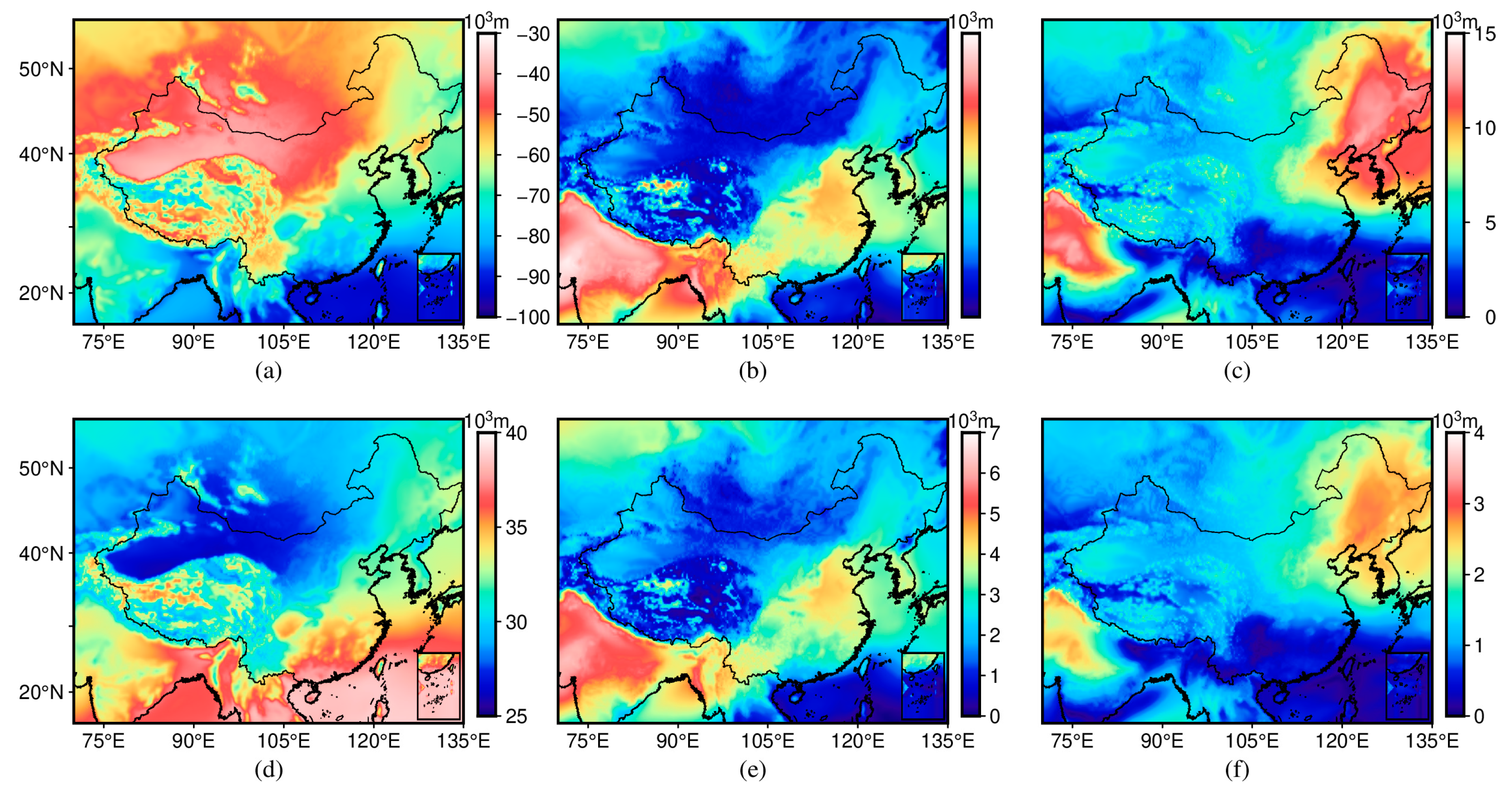
2.3. Analysis of the Gaussian Coefficient

A detailed investigation of the spatiotemporal variations of the ZTD provides important references for developing ZTD models. Direct interpolation results in large errors owing to the inconsistent heights of the four grid points. It is necessary to use appropriate functions to express the variation in ZTD with height. Hu and Yao [33] found that the Gaussian function is superior to the exponential function. Therefore, we used the Gaussian function to fit the vertical variation in ZTD, as expressed by

$$\mathrm{Z}\mathrm{T}\mathrm{D}=a·{\mathrm{e}}^{\left[-\frac{{\left(h-b\right)}^2}{c^2}\right]}$$

(5)

where h is the height (m), a is the ZTD (m) at the mean sea level, and b and c (m) are the height-scale factors (also called the Gaussian coefficients).

To verify the effectiveness of this function in expressing the vertical variation in ZTD, four representative grid points in China were selected to determine the ZTD-layered profile information from ERA5 and fitted vertical variations using the Gaussian function.

From

Table 1. The bias and RMSE of ZTD fitting curves using the Gaussian function (unit: mm).

Grid Point	50°N, 120°E	35°N, 115°E	30°N, 90°E	25°N, 110°E
bias	−7.00	−1.08	−1.63	−0.72
RMSE	14.56	10.24	10.47	8.86

, the mean bias of the four grid points was negative, indicating that a certain systematic error occurs in the Gaussian function to fit the ZTD profiles, but the value was small: approximately −1.00 mm. The root mean squared errors (RMSE) of the four grid points were 14.56, 10.24, 10.47, and 8.86 mm, respectively. From the above results, the Gaussian function attained high accuracy and stability to fit the ZTD profiles.

Analyzing the temporal variation characteristics of the Gaussian coefficients b and c is critical for developing a ZTD vertical adjustment model. Therefore, the annual mean values and amplitudes of Gaussian coefficients b and c were calculated using the ERA5 ZTD to analyze the distribution characteristics of Gaussian coefficients b and c over China. The results are shown in Figure 2. To calculate these values, the ZTD-layered profiles calculated using ERA5 atmospheric reanalysis data from 2014 to 2017 were fitted using Equation (5) to obtain b and c for all grid points. Second, the Gaussian coefficients b and c for each grid point were fitted by considering the annual and semi-annual periods using Equation (6) [20]. Finally, the annual mean values and amplitudes of Gaussian coefficients b and c were obtained using Equations (7) and (8).

$${cof}^i={\alpha }_0^i+{\alpha }_1^{i}cos\left(2\mathsf{\pi }\frac{doy}{365.25}\right)+{\alpha }_2^{i}sin\left(2\mathsf{\pi }\frac{doy}{365.25}\right)+{\alpha }_3^{i}cos\left(4\mathsf{\pi }\frac{doy}{365.25}\right)+{\alpha }_4^{i}sin\left(4\pi \frac{doy}{365.25}\right)$$

(6)

where $i$ represents the $i$-th grid point, ${cof}^i$ represents Gaussian coefficients b or c, ${\alpha }_0^i$ is the mean value of Gaussian coefficients, ${\alpha }_1^i$ to ${\alpha }_4^i$ are the period amplitude coefficients, and $doy$ is the day of the year.

$${amp}_a=\sqrt{{\left({\alpha }_1\right)}^2+{\left({\alpha }_2\right)}^2}$$

(7)

$${amp}_s=\sqrt{{\left({\alpha }_3\right)}^2+{\left({\alpha }_4\right)}^2}$$

(8)

where ${amp}_a$ represents the annual period amplitude (m) of b and c and ${amp}_s$ represents the semi-annual period amplitude (m) of b and c.

As shown in Figure 2, the characteristics of the Gaussian coefficient b varied across different regions. The annual mean values of the Gaussian coefficient b were larger in northwest China and smaller in southeast China, showing a decreasing trend from northwest to southeast China. The annual period amplitude gradually decreased from north to south, and there was a sudden increase in the Tibetan Plateau. This phenomenon may be caused by climatic differences between northern and southern China and differences between the ocean and land. The regional variation characteristics of the amplitude of the semi-annual period amplitude were subtle. In addition, the regional distribution characteristics of the annual mean values and amplitudes of Gaussian coefficient c were similar to those of Gaussian coefficient b. The annual mean values of Gaussian coefficient c showed an apparent regional variation law, as did the annual period amplitude, whereas the regional variation law of the semi-annual period amplitude was also subtle. Because the period characteristics of Gaussian coefficients b and c varied considerably across different regions, the delicate periods of Gaussian coefficients b and c must be considered for each grid point when developing a ZTD vertical adjustment model.

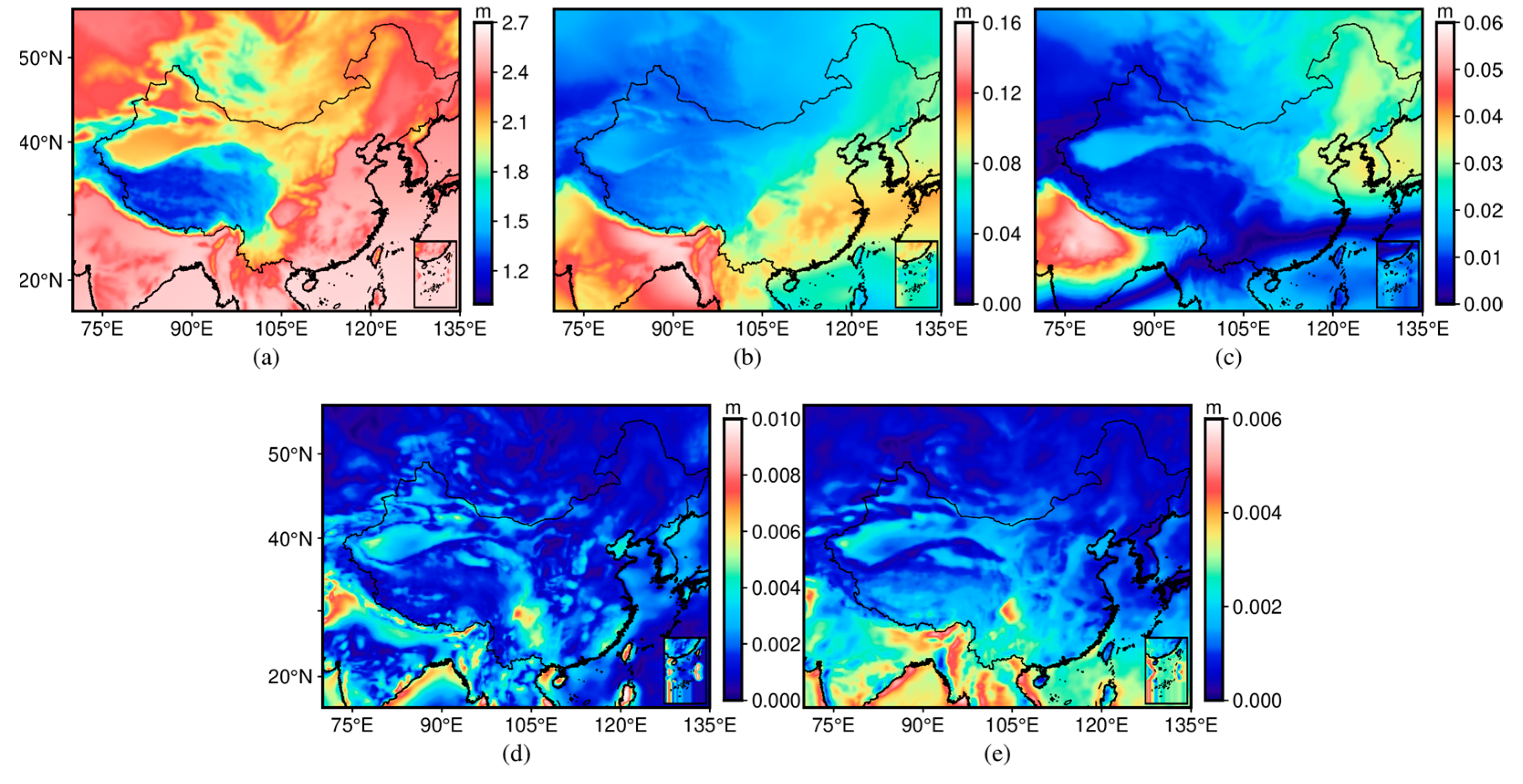
2.4. Analysis of the Surface ZTD

Analyzing the delicate temporal variations of ZTD contributes to the provision of important references for optimizing the ZTD model. The surface ZTD has significant annual and semi-annual periods [34]. Two representative grid points in China were selected to determine the diurnal and semi-diurnal periods by adopting the fast Fourier transform.

As shown in Figure 3, the surface ZTD exhibited significant diurnal and semi-diurnal period variations. The diurnal variation trends of the surface ZTD for the two grid points were different. For the first grid point, the surface ZTD increased and then decreased throughout the day, whereas the second grid point showed the opposite result. The diurnal period variation characteristics of the first grid point were significantly stronger than those of the semi-diurnal period, whereas the diurnal and semi-diurnal period variation characteristics of the second grid point were comparable. Therefore, annual, semi-annual, diurnal, and semi-diurnal periods must be considered when developing a ZTD grid model.

As shown in Figure 4, the annual mean surface ZTD was larger on the Tibetan Plateau and smaller elsewhere, which may be due to altitudinal differences. The annual period amplitude of the surface ZTD showed a decreasing trend from southeast to northwest, which may be because the northwest is far from the ocean and the southeast is close to the ocean, resulting in a large difference in the type of climate. The semi-annual period amplitude of the ZTD did not exhibit an apparent variation law. The distributions of the diurnal and semi-diurnal period amplitudes were similar. Therefore, these results further demonstrate that the delicate period of the ZTD must be considered when developing a ZTD grid model.

3. Results

3.1. Development of the NGZTD-H Model

According to the above analysis, both Gaussian coefficients b and c have annual and semi-annual period characteristics. Therefore, these coefficients of each ERA5 grid point were fitted by considering the annual and semi-annual periods. Five coefficients were calculated using Equation (6), which were stored in grid points with a horizontal resolution of 0.25° × 0.25°. After obtaining Gaussian coefficients b and c, the ZTD was adjusted vertically using the following formula [33]:

$${\mathrm{Z}\mathrm{T}\mathrm{D}}_{\mathrm{t}}={\mathrm{Z}\mathrm{T}\mathrm{D}}_{\mathrm{r}}·{\mathrm{e}}^{\left[\frac{{\left(h_{\mathrm{r}}-b\right)}^2-{\left(h_{\mathrm{t}}-b\right)}^2}{c^2}\right]}$$

(9)

where $h_{\mathrm{r}}$ and $h_{\mathrm{t}}$ are the starting and target heights (m), respectively, and ${\mathrm{Z}\mathrm{T}\mathrm{D}}_{\mathrm{r}}$ and ${\mathrm{Z}\mathrm{T}\mathrm{D}}_{\mathrm{t}}$ are the ZTD values (m) of the starting and target heights.

The ZTD vertical profile model (NGZTD-H model) consists of Equations (6) and (9). This model requires the following simple steps for application. First, after extracting the five model coefficients of the given grid point and inputting the $doy$, the Gaussian coefficients b and c were calculated using Equation (6). Second, after inputting the starting and target heights, the ZTD of the target height was calculated using Equation (9). The NGZTD-H model can achieve vertical adjustment of the ZTD from the starting height to the target height before horizontal interpolation, which reduces the interpolation errors.

To validate the NGZTD-H model, the effectiveness of vertical interpolation was evaluated using ERA5 and radiosonde data.

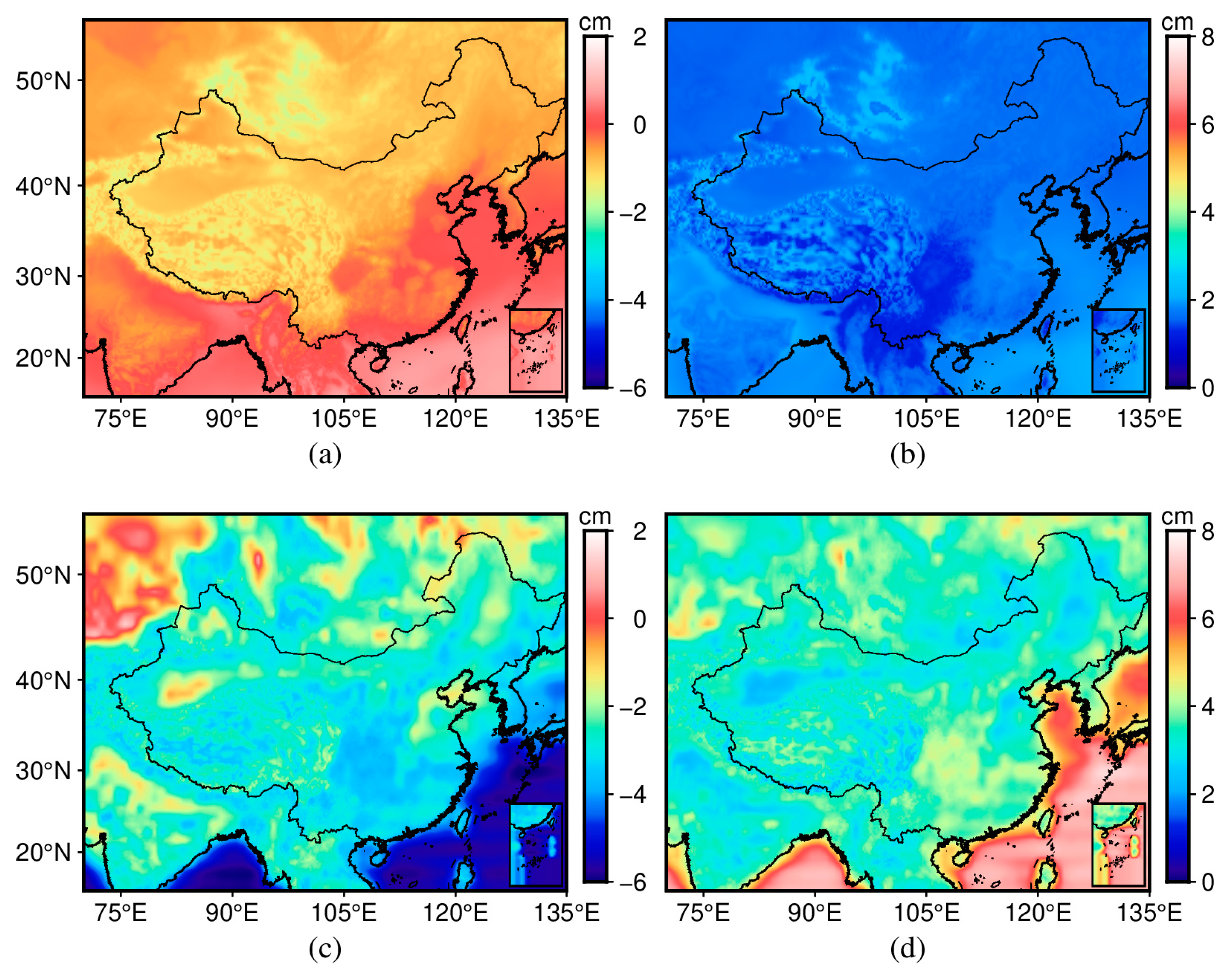
3.1.1. Accuracy Validation in ZTD Vertical Interpolation Using ERA5 Data

The proposed vertical profile model (NGZTD-H model) and the GPT3 model were evaluated using the ZTD layered profile information from ERA5 in 2018 over China. The UNB3 model can adjust the ZHD and ZWD from sea-level height to the target height. The GPT3 model provides the meteorological parameters required for the UNB3 model. Therefore, combining the GPT3 and UNB3 models can achieve a vertical adjustment for the ZTD. As the ERA5-layered ZTD recognized as a reference value does not start from sea-level height, it is necessary to derive the UNB3 model such that it can achieve vertical adjustment for ZHD and ZWD at any starting height. The derived formulas of the UNB3 model are as follows:

$${\mathrm{Z}\mathrm{H}\mathrm{D}}_{\mathrm{t}}={\mathrm{Z}\mathrm{H}\mathrm{D}}_{\mathrm{r}}{\left[1-\frac{\beta \left(H_t-H_r\right)}{T_0-\beta H_r}\right]}^{\frac{g}{R_d\beta }}$$

(10)

$${\mathrm{Z}\mathrm{W}\mathrm{D}}_{\mathrm{t}}={\mathrm{Z}\mathrm{W}\mathrm{D}}_{\mathrm{r}}{\left[1-\frac{\beta \left(H_t-H_r\right)}{T_0-\beta H_r}\right]}^{\frac{g{\lambda }^{\prime }}{R_d\beta }-1}$$

(11)

where the subscript letters t and r represent the target and the starting heights, $\beta$ is the lapse rate of temperature, $T_0$ is the thermodynamic temperature (K), $R_d$ is the dry gas constant with values of 287.0538 J·kg⁻¹, $g$ represents the ground gravity acceleration, and ${\lambda }^{\prime }$ is the water vapor lapse rate.

The NGZTD-H model was used to adjust the ZTD vertically from the surface to the ERA5 layer height. Because the GPT3 model cannot vertically adjust the ZTD directly, the surface ZHD and ZWD derived from the ERA5 data at the grid point need to be adjusted vertically and then the ZHD and ZWD must be added together to obtain the ZTD. Bias and RMSE were recognized as precision criteria. The bias and RMSE results of the NGZTD-H and GPT3 models are presented in

Table 2. Statistics of vertical interpolation accuracy for NGZTD-H model and GPT3 model using ERA5 profile ZTD in 2018 (unit: cm).

Model	NGZTD-H		GPT3
	Bias	RMSE	Bias	RMSE
Maximum	1.23	2.55	1.56	7.54
Minimum	−1.89	0.81	−6.24	1.63
Mean	−0.45	1.70	−3.02	4.01

.

As shown in Table 2, the mean bias of the NGZTD-H model and the GPT3 model were 0.45 and −3.02 cm, which indicated that the GPT3 model exhibits a larger systematic error. Furthermore, the mean RMSE of NGZTD-H model was 1.70. Compared with the GPT3 model, the accuracy of NGZTD-H model improved by 10% over the ERA5 ZTD profile. Therefore, the NGZTD-H model exhibits better stability for vertically adjusting the ZTD.

The two models were used to calculate the hourly layered ZTD at the ERA5 grid points and then to calculate the annual mean bias and RMSE to analyze the geographic distribution of the accuracy. A is shown in Figure 5. The bias of the NGZTD-H model was approximately 0 cm in most regions, negative in high-elevation regions, and positive in marine regions. The bias of the GPT3 model was positive at high latitudes and negative at low latitudes, especially in the marine regions, where it showed a large negative bias of approximately −5 cm. In addition, the RMSE of the NGZTD-H model was approximately 2 cm and no more than 3 cm in most regions, attaining a better performance in Southwest China. The GPT3 model exhibited low accuracy both in land and marine regions.

To analyze the effectiveness of the NGZTD-H model in different atmospheric pressure layers and latitudes, the ERA5-layered ZTD was also recognized as a reference value in 2018 over China. Five pressure levels were selected to evaluate the model. In addition, the Chinese region was divided into four latitude zones at 10° intervals. Finally, the accuracy of the two models were validated for the selected pressure layers and latitude bands.

As shown in Figure 6, the NGZTD-H model exhibited a small bias value in all pressure layers, positive values in two pressure layers at 800 and 200 hPa, and a negative value in the rest of the pressure layers, which were all approximately 0 cm. The GPT3 model exhibited a large value in all pressure layers; the value reached −5 cm in the pressure layers with 600 and 400 hPa. The bias of the GPT3 model was negative in all pressure layers, indicating a negative systematic error. Moreover, the RMSE of the NGZTD-H model was approximately 2 cm for all the pressure layers. It attained a better performance in 200 and 10 hPa pressure layers, which indicated that the NGZTD-H model is more precise at larger vertical interpolation heights. However, the GPT3 model exhibited larger errors in most pressure layers, with an RMSE of approximately 5 cm. In addition, the bias of the NGZTD-H model was within 1 cm for all latitude bands. The bias of the GPT3 model reached −4 cm at lower latitudes. This finding may be due to the variations of meteorological parameters in the troposphere being more complicated at low latitudes, which causes difficulties in capturing their variations using the GPT3 model. The bias of the GPT3 model also showed a decreasing trend with increasing latitude. Additionally, The NGZTD-H model exhibited good stability in all latitude bands, and its RMSE ranged from 1.5 to 2 cm. The RMSE of the GPT3 model reached 5 cm at lower latitudes. Therefore, compared with the GPT3 model, the NGZTD-H model is more suitable for the vertical adjustment of the ZTD over China.

3.1.2. Accuracy Validation in ZTD Vertical Interpolation Using Radiosonde Data

The layered ZTD at radiosonde stations in 2018 over China were considered as reference values to further validate the effectiveness of the NGZTD-H model. The ZTD at the radiosonde station was the starting value for the NGZTD-H model. The surface ZHD and ZWD at the radiosonde station were the starting values for the GPT3 model. The ZHD and ZWD, adjusted vertically using the GPT3 model, were added together to obtain the layered ZTD, which was used for comparison with the NGZTD-H model. The Gaussian coefficients b and c required for the two models at the radiosonde stations were calculated via interpolation from four ERA5 grid points around the radiosonde stations. Finally, the two models were used to calculate the layered ZTD for radiosonde stations over China at UTC 00:00 and 12:00 in 2018.

Table 3. Statistics of vertical interpolation accuracy for the NGZTD-H and GPT3 models using ZTD-layered profiles at radiosonde stations in 2018 (unit: cm).

Model	NGZTD-H		GPT3
	Bias	RMSE	Bias	RMSE
Maximum	5.09	5.31	2.25	8.68
Minimum	−3.29	1.82	−7.68	1.63
Mean	−0.32	3.10	−2.66	3.97

shows the mean bias of the NGZTD-H and GPT3 models were −0.32 and −2.66 cm, respectively, indicating that the ZTD from radiosonde stations was larger than the ZTD calculated by the GPT3 model. The mean RMSE of the NGZTD-H and GPT3 models were 3.10 and 3.97 cm. Compared with the GPT3 model, the accuracy of the NGZTD-H model enhanced by 0.87 cm (22%). The NGZTD-H model had a higher accuracy for the vertical adjustment of the ZTD. Compared with the validation results using the ERA5 profile ZTD, the NGZTD-H model exhibited lower accuracy, which may be due to the interpolation errors of Gaussian coefficients from four grid points to the radiosonde stations.

As is shown in Figure 7, the bias of the NGZTD-H model was small at all radiosonde stations and approximately 0 cm in most regions. Both the NGZTD-H and GPT3 models exhibited a large positive bias at higher elevations in southwest China, which may be due to the undulating terrain. The bias of the GPT3 model reached −8 cm at certain stations, indicating that serious systematic errors occur in the GPT3 model. In addition, the RMSE of the NGZTD-H model was stable without abrupt variations. At higher latitudes, the difference in RMSE between the NGZTD-H and GPT3 models was small. The GPT3 model exhibited a larger RMSE at low latitudes for the reasons noted earlier.

To investigate the adaptability of the NGZTD-H model to seasonal variation, the diurnal mean bias and RMSE were determined at two representative radiosonde stations (Hailar and Hangzhou). As shown in Figure 8, at the Hailar radiosonde station, the GPT3 model, which had poor seasonal adaptation, was seriously affected by seasonal variations, and its bias fluctuated throughout the year. However, the NGZTD-H model could resist the influence of the season on the vertical adjustment of the ZTD, and its bias was stable throughout the year. The RMSE of the new model was 2 cm. At the Hangzhou radiosonde station, two models exhibited fluctuations. The bias of the NGZTD-H model fluctuated at approximately 0 cm, and its RMSE was approximately 2 cm. However, the GPT3 model exhibited a more evident negative bias. Therefore, the NGZTD-H model is more suitable for capturing seasonal variations than the GPT3 model.

Because the vertical adjustment of the ZTD is related to elevation, the radiosonde stations over China were divided into five intervals to validate the effectiveness of the NGZTD-H model at different elevations. Figure 9 shows the bias and RMSE statistics in each interval for the NGZTD-H and GPT3 models. The GPT3 model exhibited a larger positive bias in the interval of 3–4 km and a larger negative bias in the intervals of 0–3 and >4 km. The bias of the NGZTD-H model was smaller in each interval. A larger positive bias occurred in the interval of 3–4 km, indicating that the NGZTD-H model had a larger value than the reference value in this interval. Furthermore, the RMSE of the GPT3 model was larger in the intervals of 0–1 and 2–3 km. The above analysis shows the NGZTD-H model exhibited more stable performances in vertical adjustment for ZTD over China.

3.2. Development of the NGZTD Model

From the above analysis of spatiotemporal characteristics, the surface ZTD exhibited regular seasonal and diurnal variations. Therefore, the development of a ZTD model must consider the delicate periods of the surface ZTD. This equation is expressed as follows:

$$\begin{gathered} {\mathrm{Z}\mathrm{T}\mathrm{D}}_{\mathrm{s}}^i={\alpha }_0^i+{\alpha }_1^{i}cos\left(2\mathsf{\pi }\frac{doy}{365.25}\right)+{\alpha }_2^{i}sin\left(2\mathsf{\pi }\frac{doy}{365.25}\right)+{\alpha }_3^{i}cos\left(4\mathsf{\pi }\frac{doy}{365.25}\right)+{\alpha }_4^{i}sin\left(4\mathsf{\pi }\frac{doy}{365.25}\right)+{\alpha }_5^{i}cos\left(2\mathsf{\pi }\frac{hod}{24}\right) \\ +{\alpha }_6^{i}sin\left(2\mathsf{\pi }\frac{hod}{24}\right)+{\alpha }_7^{i}cos\left(4\mathsf{\pi }\frac{hod}{24}\right)+{\alpha }_8^{i}sin\left(4\mathsf{\pi }\frac{hod}{24}\right) \end{gathered}$$

(12)

where ${\mathrm{Z}\mathrm{T}\mathrm{D}}_{\mathrm{s}}^i$ is the surface ZTD (m), ${\alpha }_0^i$ is the annual mean ZTD, ${\alpha }_1^i$ to ${\alpha }_8^i$ are the period amplitude coefficients, and $hod$ is the hour (UTC) of day.

The surface ZTD of all ERA5 grid points over China from 2014 to 2017 was used to calculate nine coefficients using the least squares method. The new ZTD grid model (NGZTD model), which directly calculates the ZTD, consists of Equation (12) and the NGZTD-H model proposed earlier. The method for using the NGZTD model is as follows: First, the user’s coordinates are determined to search the ERA5 grid points around the user. After the model coefficients of these grid points have been obtained, as shown in Equation (12), the surface ZTD can be calculated by inputting $doy$ and $hod$ using Equation (12). Second, the NGZTD-H model is employed to calculate ZTD at the height as the user after obtaining the Gaussian coefficients b and c. Finally, the user’s ZTD is calculated using inverse distance interpolation. The NGZTD model was developed based on high-resolution ERA5 data, employs the high-precision Gaussian function to adjust the ZTD vertically, and considers seasonal and delicate diurnal variations in the ZTD, which ensures the effectiveness of the model. Furthermore, the NGZTD model has the advantages of efficiency and simplicity because measured meteorological parameters are not required, and the model coefficients are fewer in number and are stored in regular grid points.

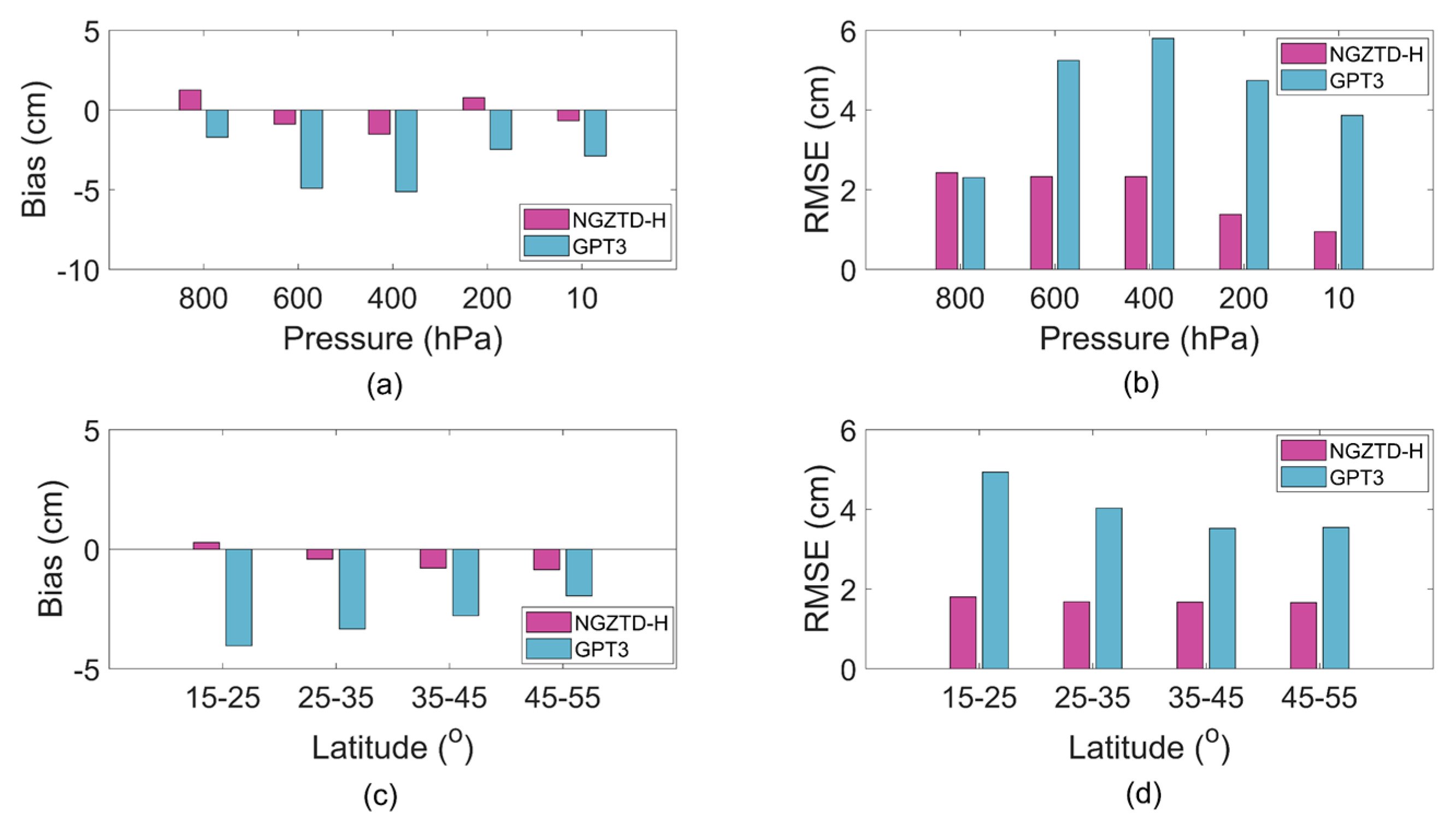
3.2.1. Accuracy Validation Using GNSS Data

The effectiveness of the NGZTD model for estimating the ZTD was validated using the GNSS-derived ZTD in 2018 over China. Because the NGZTD model estimated the ZTD based on the ERA5 grid points, the GNSS and ERA5 data were unified with the same elevation system. The ZTD with a temporal resolution of 1 h at the GNSS stations was determined using both the NGZTD and GPT3 models, and the results were compared with the GNSS-derived ZTD. The accuracy statistics for the two models are presented in

Table 4. Statistics of accuracy for NGZTD and GPT3 models using GNSS-derived ZTD in 2018 (unit: cm).

Model	NGZTD		GPT3
	Bias	RMSE	Bias	RMSE
Maximum	1.06	7.79	3.96	7.92
Minimum	−3.98	1.15	−2.82	1.38
Mean	−0.38	3.38	0.16	4.33

and Figure 10.

As shown in Table 4, the mean bias of the GPT3 model was −0.38 cm and 0.16 cm. The ZTD calculated by the NGZTD model was generally smaller than the GNSS-derived ZTD but generally larger than the reference value for the GPT3 model. The bias of the NGZTD model was −0.38 cm and ranged from −3.98 to 1.06 cm, and the negative bias was larger, which indicated that some of the ZTD calculated by the NGZTD model were much smaller than the GNSS-derived ZTD. The NGZTD and GPT3 models had a similar RMSE range from 1 cm to 8 cm. The mean RMSE of the two models were 3.38 and 4.33 cm, respectively. Compared with the GPT3 model, the NGZTD model achieved an improvement of 0.95 cm (22%).

As shown in Figure 10, the bias of the GPT3 model was positive in the western and southwestern regions and negative in the eastern region, indicating that the performance of this model was unstable. The NGZTD model performed better than the other regions in northern China. Especially in western and southwestern China with undulating terrain, the NGZTD model exhibited better stability, indicating that the NGZTD model is more adaptable to the influence of complex geographical conditions. The NGZTD model exhibited a stable performance with an RMSE of approximately 2 cm. However, the GPT3 model exceeded 2 cm in most regions of China and reached 6 cm in the eastern region. The two models do not perform well in the eastern region, which may be affected by atmospheric differences between the sea and land.

To investigate the season adaptation of the NGZTD model, two representative GNSS stations (Kuqa and Delingha) were selected as validation stations. The diurnal mean bias and RMSE results are shown in Figure 11. The GPT3 model exhibited positive bias at both GNSS stations Kuqa and Delingha, whereas the NGZTD model exhibited smaller and more stable bias during the entire year. The NGZTD model performed a better result with an RMSE below 4 cm, indicating that the new ZTD model can cope with the influences of season.

ZTD is affected by the season as well as delicate diurnal variations. Two GNSS stations, Kuqa and Guilin, were selected to investigate the effectiveness of the NGZTD model to capture diurnal variations in the ZTD. The hourly ZTD over a five-day period in 2018 was estimated by both the NGZTD and GPT3 models, and their results were compared with the GNSS-derived ZTD and are shown in Figure 12. At the Kuqa GNSS station, the GNSS-derived ZTD ranged from 2.08 to 2.09 cm, exhibiting a diurnal period during those five days. The ZTD estimated by the NGZTD model also exhibited a diurnal period and agreed well with the reference value, indicating that the NGZTD model can capture the delicate diurnal variation of the ZTD. However, the ZTD determined using the GPT3 model was the same for one day and was larger than the reference value. At the Guilin GNSS station, although the ZTD calculated by the GPT3 model was close to the GNSS-derived ZTD, this model was not able to capture the diurnal variation in the ZTD. Therefore, the proposed model can capture both seasonal and diurnal variations in the ZTD.

3.2.2. Accuracy Validation Using Radiosonde Data

Layered ZTD at radiosonde stations in 2018 over China were considered as reference data to validate the accuracy of the NGZTD model. To investigate the contribution of considering the seasonal variations of Gaussian coefficients b and c to the accuracy of estimating ZTD, the proposed model, which considered the seasonal variations of Gaussian coefficients and took the constants b and c as −7000 and 30,000 m, respectively, was used to calculate the layered ZTD at radiosonde stations at 00:00 and 12:00 and compared the results with those of the GPT3 model.

As shown in

Table 5. Statistics of accuracy for the NGZTD model, the model with constant Gaussian coefficients, and the GPT3 model using the ZTD-layered profiles at radiosonde stations in 2018 (unit: cm).

Model	NGZTD		The Model with Constant Gaussian Coefficients		GPT3
	Bias	RMSE	Bias	RMSE	Bias	RMSE
Maximum	2.16	5.36	−0.26	9.51	4.80	6.47
Minimum	−4.31	1.58	−9.5	2.51	−2.74	2.91
Mean	−1.53	3.62	−4.63	5.91	0.32	5.25

, the mean bias of the NGZTD model and the model with constant Gaussian coefficients were −1.53 and −4.63 cm, respectively, and the ZTD estimated by the NGZTD model with constant Gaussian coefficients showed an evident difference from the reference value, which indicated that seasonal variations in Gaussian coefficients need to be considered. The GPT3 model exhibited a more stable performance with a mean bias of 0.32 cm. The mean RMSE of the NGZTD model, the model with constant Gaussian coefficients, and the GPT3 model were 3.62, 5.91, and 5.25 cm, respectively. The NGZTD model achieved the highest accuracy, with an improvement of 2.29 (39%) and 1.63 cm (31%) compared with the other models. Therefore, these results further indicated that considering seasonal variations in the Gaussian coefficients contributed to the effectiveness of the NGZTD model.

Figure 13 shows that the NGZTD model exhibited a negative bias at most stations, whereas the GPT3 model exhibited a positive bias. The RMSE of the GPT3 model exceeded 5 cm in most regions. In particular, in regions with high altitudes and undulating terrain, the NGZTD model is more advantageous. In addition, Figure 14 shows the accuracy percentage for the NGZTD and GPT3 models. The NGZTD model had the largest proportion of RMSE in the interval of 2–3 cm, accounting for 30% of the RMSE, whereas the largest proportion of RMSE for the GPT3 model was in the interval of 5–6 cm, accounting for 69% of the RMSE. In the interval in which the RMSE was <2 cm, the NGZTD model accounted for 2%, whereas the GPT3 model accounted for 0%. According to the above results of the accuracy validation, the NGZTD model exhibited stable and high accuracy in terms of capturing seasonal and diurnal variations, adaptability to terrain, and adaptability to different elevations. The new ZTD model can directly provide reliable and high-precision ZTD for users in China.

4. Discussion

As shown in Table 2, Table 4 and Table 5, the mean RMSE of the vertical interpolation for the NGZTD-H model was 1.70 cm when the ERA5 data were used as the reference value, whereas the mean RMSE of the NGZTD model for the direct calculation of the ZTD exceeded 3 cm when both the GNSS data and radiosonde data were used as the reference value. Unlike the vertical interpolation validation for the NGZTD-H model in Section 3.1.1, the starting ZTD for the NGZTD model in Section 3.2.1 and Section 3.2.2. was obtained by a model considering the seasonal and diurnal variations of ZTD, whereas the starting ZTD in Section 3.1.1. was obtained by the integral method. In addition, the NGZTD model required horizontal interpolation to calculate the ZTD at GNSS and radiosonde stations in Section 3.2.1 and Section 3.2.2. Based on the above analysis, the errors of the NGZTD model may be attributed to the starting ZTD and horizontal interpolation.

To validate the above error sources, the GNSS-derived ZTD in 2018 over China was used to validate the spatial interpolation accuracy for the NGZTD-H model. First, the Gaussian coefficients b and c were determined. Second, the ZTD on the ERA5 grid points was vertically adjusted to the GNSS station height using the NGZTD-H model. It should be noted that the starting ZTD on the ERA5 grid points was obtained by the integral method. Finally, the adjusted ZTD was interpolated horizontally to the GNSS station employing an inverse distance interpolation method. A comparison of the interpolated results with the GNSS-derived ZTD validated the effectiveness of the NGZTD-H model. Because the elevations of GNSS stations are geodesic heights and the elevations of ERA5 grid points are geopotential heights, it is necessary to unify the elevations of these two products before vertically adjusting the ZTD. In this study, we employed the EGM2008 model [45] to convert elevations of the ERA5 data to geodesic elevations.

The spatial interpolation accuracy of the NGZTD-H model was compared with that of the GPT3 model. The mean bias of the GPT3 model was −1.14 cm (

Table 6. Statistics of spatial interpolation accuracy for NGZTD-H and GPT3 models using GNSS-derived ZTD in 2018 (unit: cm).

Model	NGZTD-H		GPT3
	Bias	RMSE	Bias	RMSE
maximum	1.36	8.14	1.23	8.57
minimum	−3.10	0.66	−3.28	0.95
mean	−0.56	1.48	−1.14	1.79

). This indicated the GPT3 model had certain systematic errors. The bias intervals of the two models were similar; both ranged from −3 to 1 cm. The mean RMSE of the NGZTD-H and GPT3 models were 1.48 cm and 1.79 cm. Compared with the GPT3 model, the accuracy of the NGZTD-H model improved by 0.31 cm (17%). Therefore, the NGZTD-H model has higher accuracy for the spatial interpolation of the ZTD.

Figure 15 shows the stable results for NGZTD-H model at each GNSS station in China. Its bias was approximately 0 cm in most regions and reached −3 cm at individual stations in Southwest China, which indicated that the model struggles to express the vertical variation of ZTD in these regions. However, the result of the GPT3 model shows a large negative bias in most regions. The RMSE of the NGZTD-H model was smaller at high latitudes. However, the RMSE of the GPT3 model was greater than 2 cm at most GNSS stations. Therefore, compared with the GPT3 model, the NGZTD-H model has better stability in spatial interpolation.

The mean RMSE of spatial interpolation for the NGZTD-H model was 1.48 cm, which was apparently smaller than that of the NGZTD model in Section 3.2.1 and Section 3.2.2. The validation of spatial interpolation accuracy for the NGZTD-H model used ZTD obtained by the integral method as the starting ZTD and required horizontal interpolation. This indicated that the errors of the NGZTD model mainly derive from the starting ZTD rather than from horizontal interpolation.

As shown in Table 2 and Table 6, the spatial interpolation accuracy (the mean RMSE was 1.48 cm) of the NGZTD-H model is higher than the vertical interpolation accuracy (the mean RMSE was 1.70 cm). The validation of spatial interpolation accuracy for the NGZTD-H model required horizontal interpolation, whereas this is not required for vertical interpolation in Section 3.1.1. This further indicated that the errors caused by horizontal interpolation were relatively small. According to the above analysis, the accuracy of ZTD vertical adjustment was higher in flat-terrain regions and lower in western China with undulating terrain. The GNSS stations are fewer in western China, whereas the distribution of ERA5 grid points is uniform, which resulted in a higher number of GNSS stations with smaller errors. Therefore, the accuracy of the spatial interpolation for the NGZTD-H model was higher than that of the vertical interpolation in Section 3.1.1.

5. Conclusions

To overcome the limitations of existing ZTD models that lack an appropriate vertical adjustment function and are unsuitable for use in China in light of its complex climate and greatly undulating terrain, this study proposed an NGZTD model considering time-varying vertical adjustment based on the Gaussian function and diurnal variation. First, a ZTD vertical adjustment model, NGZTD-H, was developed that can adjust the ZTD from the starting height to the target height. Then, an NGZTD model that considers the seasonal and delicate diurnal variation in the ZTD was developed to estimate the ZTD directly. The vertical interpolation accuracy of the NGZTD-H model was validated, and the model exhibited stability for different geographic regions, pressure layers, latitudes, seasons, and elevations. The NGZTD model was validated using GNSS-derived ZTD and layered ZTD at radiosonde stations, and the results show that the NGZTD model performed better than the GPT3 model in time and space dimensions. In particular, in terms of capturing diurnal variation, the NGZTD model can effectively detect diurnal variation in the ZTD. Because the NGZTD model adopted the Gaussian function to adjust the ZTD vertically, the new model exhibited a more stable performance than the GPT3 model in western and southwestern China, where the terrain is undulating. Seasonal variations in Gaussian coefficients need to be considered. Using constant Gaussian coefficients will generate large errors. Finally, the error sources of the NGZTD model were discussed, which indicated that the starting ZTD was the main error source. In the future, we will further overcome the error sources of the NGZTD model to improve its accuracy and apply the proposed NGZTD model to precise point positioning and InSAR technology. The proposed model is expected to provide a reference for studying tropospheric parameters.

References

1. Yao, Y.B.; He, C.Y.; Zhang, B.; Xu, C.Q. A New Global Zenith Tropospheric Delay Model GZTD. Chin. J. Geophys. 2013, 56, 2218–2227. [Google Scholar]
2. Shi, C.; Wang, H.S.; Cao, Y.C.; Zhang, E.H.; Liang, H.; Fu, Z.K. Analysis on Performance of Water Vapor Detection Based on BeiDou Satellite. Geomat. Inf. Sci. Wuhan Univ. 2016, 41, 285–289. [Google Scholar]
3. Vedel, H.; Mogensen, K.; Huang, X. Calculation of Zenith Delays from Meteorological Data Comparison of NWP Model, Radiosonde and GPS Delays. Phys. Chem. Earth 2001, 26, 497–502. [Google Scholar] [CrossRef]
4. Li, H.B.; Wang, X.M.; Wu, S.Q.; Zhang, K.F.; Chen, X.L.; Zhang, J.L.; Qiu, C.; Zhang, S.T.; Li, L. An Improved Model for Detecting Heavy Precipitation Using GNSS-Derived Zenith Total Delay Measurements. IEEE J. Sel. Top. Appl. Earth Obs. Remote Sens. 2021, 14, 5392–5405. [Google Scholar] [CrossRef]
5. Yang, Y.F.; Chen, X.P.; Yao, M.H.; Zhou, C.L.; Liao, C.M. Research on Zenith Tropospheric Delay Modeling of Regional Cors Network. Int. Arch. Photogramm. Remote Sens. Spat. Inf. Sci. 2020, 42, 1197–1200. [Google Scholar] [CrossRef]
6. Hopfield, H. Two-quartic Tropospheric Refractivity Profile for Correcting Satellite Data. J. Geophys. Res. 1969, 74, 4487–4499. [Google Scholar] [CrossRef]
7. Saastamoinen, J. Atmospheric Correction for the Troposphere and Stratosphere in Radio Ranging Satellites. Use Artif. Satell. Geod. 1972, 15, 247–251. [Google Scholar]
8. Black, H.D. An Easily Implemented Algorithm for the Tropospheric Range Correction. J. Geophys. Res. Solid Earth 1978, 83, 1825–1828. [Google Scholar] [CrossRef]
9. Yao, Y.B.; Hu, Y.F.; Yu, C.; Zhang, B.; Guo, J.J. An Improved Global Zenith Tropospheric Delay Model GZTD2 Considering Diurnal Variations. Nonlinear Process. Geophys. 2016, 23, 127–136. [Google Scholar] [CrossRef]
10. Penna, N.; Dodson, A.; Chen, W. Assessment of EGNOS Tropospheric Correction Model. J. Navig. 2001, 54, 37–55. [Google Scholar] [CrossRef]
11. Leandro, R.F.; Langley, R.B.; Santos, M.C. UNB3m_pack: A Neutral Atmosphere Delay Package for Radiometric Space Techniques. GPS Solut. 2008, 12, 65–70. [Google Scholar] [CrossRef]
12. Schüler, T. The TropGrid2 Standard Tropospheric Correction Model. GPS Solut. 2014, 18, 123–131. [Google Scholar] [CrossRef]
13. Böhm, J.; Heinkelmann, R.; Schuh, H. Short Note: A Global Model of Pressure and Temperature for Geodetic Applications. J. Geod. 2007, 81, 679–683. [Google Scholar] [CrossRef]
14. Lagler, K.; Schindelegger, M.; Böhm, J.; Krásná, H.; Nilsson, T. GPT2: Empirical Slant Delay Model for Radio Space Geodetic Techniques. Geophys. Res. Lett. 2013, 40, 1069–1073. [Google Scholar] [CrossRef] [PubMed]
15. Böhm, J.; Möller, G.; Schindelegger, M.; Pain, G.; Weber, R. Development of an Improved Empirical Model for Slant Delays in the Troposphere (GPT2w). GPS Solut. 2015, 19, 433–441. [Google Scholar] [CrossRef]
16. Landskron, D.; Böhm, J. VMF3/GPT3: Refined Discrete and Empirical Troposphere Mapping Functions. J. Geod. 2018, 92, 349–360. [Google Scholar] [CrossRef]
17. Sun, Z.Y.; Zhang, B.; Yao, Y.B. An ERA5-based Model for Estimating Tropospheric Delay and Weighted Mean Temperature over China with Improved Spatiotemporal Resolutions. Earth Space Sci. 2019, 6, 1926–1941. [Google Scholar] [CrossRef]
18. Ding, J.S.; Chen, J.P. Assessment of Empirical Troposphere Model GPT3 Based on NGL’s Global Troposphere Products. Sensors 2020, 20, 3631. [Google Scholar] [CrossRef]
19. Li, W.; Yuan, Y.B.; Ou, J.K.; Li, H.; Li, Z.S. A New Global Zenith Tropospheric Delay Model IGGtrop for GNSS Applications. Chin. Sci. Bull. 2012, 57, 2132–2139. [Google Scholar] [CrossRef]
20. Huang, L.K.; Zhu, G.; Peng, H.; Liu, L.L.; Ren, C.; Jiang, W.P. An Improved Global Grid Model for Calibrating Zenith Tropospheric Delay for GNSS Applications. GPS Solut. 2023, 27, 17. [Google Scholar] [CrossRef]
21. Zhou, F.; Cao, X.Y.; Ge, Y.L.; Li, W.W. Assessment of the Positioning Performance and Tropospheric Delay Retrieval with Precise Point Positioning Using Products from Different Analysis Centers. GPS Solut. 2020, 24, 12. [Google Scholar] [CrossRef]
22. Xiong, C.B.; Yu, L.N.; Zhao, L.W. Analysis on the Impacts of Slant Tropospheric Delays on Precise Point Positioning. Appl. Sci. 2019, 9, 4884. [Google Scholar] [CrossRef]
23. Yao, Y.B.; Xu, X.Y.; Xu, C.Q.; Peng, W.J.; Wan, Y.Y. GGOS Tropospheric Delay Forecast Product Performance Evaluation and Its Application in Real-Time PPP. J. Atmos. Sol.-Terr. Phys. 2018, 175, 1–17. [Google Scholar] [CrossRef]
24. Guo, L.J.; Huang, L.K.; Li, J.Y.; Liu, L.L.; Huang, L.; Fu, B.L.; Xie, S.F.; He, H.C.; Ren, C. A Comprehensive Evaluation of Key Tropospheric Parameters from ERA5 and MERRA-2 Reanalysis Products Using Radiosonde Data and GNSS Measurements. Remote Sens. 2021, 13, 3008. [Google Scholar] [CrossRef]
25. Sun, Z.Y.; Zhang, B.; Yao, Y.B. A Global Model for Estimating Tropospheric Delay and Weighted Mean Temperature Developed with Atmospheric Reanalysis Data from 1979 to 2017. Remote Sens. 2019, 11, 1893. [Google Scholar] [CrossRef]
26. Song, S.L.; Zhu, W.Y.; Chen, Q.M.; Liou, Y.A. Establishment of a New Tropospheric Delay Correction Model over China Area. Sci. China Phys. Mech. Astron. 2011, 54, 2271–2283. [Google Scholar] [CrossRef]
27. Li, H.J.; Zhu, G.; Kang, Q.; Huang, L.K.; Wang, H. A Global Zenith Tropospheric Delay Model with ERA5 and GNSS-Based ZTD Difference Correction. GPS Solut. 2023, 27, 154. [Google Scholar] [CrossRef]
28. Huang, L.K.; Liu, L.L.; Yao, C.L. A Zenith Tropospheric Delay Correction Model Based on the Regional CORS Network. Geod. Geodyn. 2012, 3, 53–62. [Google Scholar]
29. Huang, L.K.; Zhu, G.; Liu, L.L.; Chen, H.; Jiang, W.P. A Global Grid Model for the Correction of the Vertical Zenith Total Delay Based on a Sliding Window Algorithm. GPS Solut. 2021, 25, 98. [Google Scholar] [CrossRef]
30. Huang, L.K.; Lan, S.W.; Zhu, G.; Chen, F.D.; Li, J.Y.; Liu, L.L. A Global Grid Model for the Estimation of Zenith Tropospheric Delay Considering the Variations at Different Altitudes. Geosci. Model Dev. 2023, 16, 7223–7235. [Google Scholar] [CrossRef]
31. Zhu, G.; Huang, L.K.; Yang, Y.Z.; Li, J.Y.; Zhou, L.; Liu, L.L. Refining the ERA5-Based Global Model for Vertical Adjustment of Zenith Tropospheric Delay. Satell. Navig. 2022, 3, 27. [Google Scholar] [CrossRef]
32. Sun, J.L.; Wu, Z.L.; Yin, Z.D.; Ma, B. A Simplified GNSS Tropospheric Delay Model Based on the Nonlinear Hypothesis. GPS Solut. 2017, 21, 1735–1745. [Google Scholar] [CrossRef]
33. Hu, Y.F.; Yao, Y.B. A New Method for Vertical Stratification of Zenith Tropospheric Delay. Adv. Space Res. 2019, 63, 2857–2866. [Google Scholar] [CrossRef]
34. Zhao, Q.Z.; Su, J.; Xu, C.Q.; Yao, Y.B.; Zhang, X.Y.; Wu, J.F. High-Precision ZTD Model of Altitude-Related Correction. IEEE J. Sel. Top. Appl. Earth Obs. Remote Sens. 2023, 16, 609–621. [Google Scholar] [CrossRef]
35. Dong, D.H.; Huang, G.; Qu, X.; Tao, W.C.; Fan, G.Z. Temperature Trend–Altitude Relationship in China during 1963–2012. Theor. Appl. Climatol. 2015, 122, 285–294. [Google Scholar] [CrossRef]
36. Huang, L.K.; Wang, X.; Xiong, S.; Li, J.Y.; Liu, L.L.; Mo, Z.X.; Fu, B.L.; He, H.C. High-Precision GNSS PWV Retrieval Using Dense GNSS Sites and in-Situ Meteorological Observations for the Evaluation of MERRA-2 and ERA5 Reanalysis Products over China. Atmos. Res. 2022, 276, 106247. [Google Scholar] [CrossRef]
37. Fang, J.Y.; Yu, G.R.; Liu, L.L.; Hu, S.J.; Chapin III, F.S. Climate Change, Human Impacts, and Carbon Sequestration in China. Proc. Nat. Acad. Sci. USA 2018, 115, 4015–4020. [Google Scholar] [CrossRef]
38. Dee, D.P.; Uppala, S.M.; Simmons, A.J.; Berrisford, P.; Poli, P.; Kobayashi, S.; Andrae, U.; Balmaseda, M.A.; Balsamo, G.; Bauer, P.; et al. The ERA-Interim Reanalysis: Configuration and Performance of the Data Assimilation System. Q. J. R. Meteorol. Soc. 2011, 137, 553–597. [Google Scholar] [CrossRef]
39. Jiang, C.H.; Xu, T.H.; Wang, S.M.; Nie, W.F.; Sun, Z.Z. Evaluation of Zenith Tropospheric Delay Derived from ERA5 Data over China Using GNSS Observations. Remote Sens. 2020, 12, 663. [Google Scholar] [CrossRef]
40. Chen, B.Y.; Yu, W.K.; Wang, W.; Zhang, Z.T.; Dai, W.J. A Global Assessment of Precipitable Water Vapor Derived from GNSS Zenith Tropospheric Delays with ERA5, NCEP FNL, and NCEP GFS Products. Earth Space Sci. 2021, 8, e2021EA001796. [Google Scholar] [CrossRef]
41. Sun, Y.L.; Yang, F.; Liu, M.J.; Li, Z.C.; Gong, X.; Wang, Y.Y. Evaluation of the Weighted Mean Temperature over China Using Multiple Reanalysis Data and Radiosonde. Atmos. Res. 2023, 285, 106664. [Google Scholar] [CrossRef]
42. Zhou, C.C.; Peng, B.B.; Li, W.; Zhong, S.M.; Ou, J.K.; Chen, R.J.; Zhao, X.L. Establishment of a Site-Specific Tropospheric Model Based on Ground Meteorological Parameters over the China Region. Sensors 2017, 17, 1722. [Google Scholar] [CrossRef] [PubMed]
43. Dousa, J.; Bennitt, G.V. Estimation and Evaluation of Hourly Updated Global GPS Zenith Total Delays over Ten Months. GPS Solut. 2013, 17, 453–464. [Google Scholar] [CrossRef]
44. Zhao, Q.Z.; Yang, P.F.; Yao, W.Q.; Yao, Y.B. Hourly PWV Dataset Derived from GNSS Observations in China. Sensors 2019, 20, 231. [Google Scholar] [CrossRef]
45. Zhang, C.Y.; Guo, C.X.; Chen, J.Y.; Zhang, L.; Wang, B. EGM 2008 and Its Application Analysis in Chinese Mainland. Acta Geod. Cartogr. Sin. 2009, 38, 283–289. [Google Scholar]
Figure 1. The research framework.
Remotesensing 16 02023 g001
Figure 2. Distributions of the annual mean value and period amplitudes for Gaussian coefficients b and c. (a) The annual mean value of b. (b) The annual period amplitude of b. (c) The semi-annual period amplitude of b. (d) The annual mean value of c. (e) The annual period amplitude of c. (f) The semi-annual period amplitude of c.
Remotesensing 16 02023 g002
Figure 3. The diurnal variation of the surface ZTD and its spectral analysis results. (a) 50°N, 120°E. (b) 35°N, 115°E.
Remotesensing 16 02023 g003
Figure 4. Distribution of annual mean value and period amplitudes for surface ZTD. (a) The annual mean value. (b) The annual period amplitude. (c) The semi-annual period amplitude. (d) The diurnal period amplitude. (e) The semi-diurnal period amplitude.
Remotesensing 16 02023 g004
Figure 5. Distribution of vertical interpolation accuracy for NGZTD-H model and GPT3 model using ERA5 profile ZTD in 2018. (a) The bias of NGZTD-H. (b) The RMSE of NGZTD-H. (c) The bias of GPT3. (d) The RMSE of GPT3.
Remotesensing 16 02023 g005
Figure 6. Distribution of vertical interpolation accuracy for NGZTD-H and GPT3 models in the selected pressure layers and latitude bands using ERA5 profile ZTD in 2018. (a) The bias of pressure layers. (b) The RMSE of pressure layers. (c) The bias of latitude bands. (d) The RMSE of latitude bands.
Remotesensing 16 02023 g006
Figure 7. Distribution of vertical interpolation accuracy for the NGZTD-H and GPT3 models using the ZTD-layered profiles at radiosonde stations in 2018. (a) The bias of NGZTD-H. (b) The RMSE of NGZTD-H. (c) The bias of GPT3. (d) The RMSE of GPT3.
Remotesensing 16 02023 g007
Figure 8. Distribution of vertical interpolation accuracy for NGZTD-H model and GPT3 model in different seasons using the ZTD-layered profiles at radiosonde stations in 2018. (a) Hailar. (b) Hangzhou.
Remotesensing 16 02023 g008
Figure 9. Distribution of vertical interpolation accuracy for the NGZTD-H and GPT3 models at different heights using the ZTD-layered profiles at radiosonde stations in 2018. (a) The bias. (b) The RMSEs.
Remotesensing 16 02023 g009
Figure 10. Distribution of accuracy for NGZTD and GPT3 models using the GNSS-derived ZTD at GNSS stations in 2018. (a) The bias of NGZTD. (b) The RMSE of NGZTD. (c) The bias of GPT3. (d) The RMSE of GPT3.
Remotesensing 16 02023 g010
Figure 11. Distribution of accuracy for NGZTD and GPT3 models in different seasons using GNSS-derived ZTD in 2018. (a) Kuqa. (b) Delingha.
Remotesensing 16 02023 g011
Figure 12. Distribution of accuracy for NGZTD and GPT3 models during five days using GNSS-derived ZTD in 2018. (a) Kuqa. (b) Guilin.
Remotesensing 16 02023 g012
Figure 13. Distribution of accuracy for the NGZTD model, the model with constant Gaussian coefficients, and the GPT3 model using the ZTD-layered profiles at radiosonde stations in 2018. (a) The bias of NGZTD. (b) The RMSE of NGZTD. (c) The bias of GPT3. (d) The RMSE of GPT3.
Remotesensing 16 02023 g013
Figure 14. The percentage results of the RMSE for the NGZTD and GPT3 models using the ZTD-layered profiles at radiosonde stations in 2018. (a) NGZTD model. (b) GPT3 model.
Remotesensing 16 02023 g014
Figure 15. Distribution of spatial interpolation accuracy for NGZTD-H and GPT3 models using the GNSS-derived ZTD at GNSS stations in 2018. (a) The bias of NGZTD-H. (b) The RMSE of NGZTD-H. (c) The bias of GPT3. (d) The RMSE of GPT3.
Remotesensing 16 02023 g015