Abstract
In bridge structure monitoring and evaluation, deformation data serve as a crucial basis for assessing structural conditions. Different from discrete monitoring points, spatially continuous deformation modes provide a comprehensive understanding of deformation and potential information. Terrestrial laser scanning (TLS) is a three-dimensional deformation monitoring technique that has gained wide attention in recent years, demonstrating its potential in capturing structural deformation models. In this study, a TLS-based bridge deformation mode monitoring method is proposed, and a deformation mode calculation method combining sliding windows and surface fitting is developed, which is called the SWSF method for short. On the basis of the general characteristics of bridge structures, a deformation error model is established for the SWSF method, with a detailed quantitative analysis of each error component. The analysis results show that the deformation monitoring error of the SWSF method consists of four parts, which are related to the selection of the fitting function, the density of point clouds, the noise of point clouds, and the registration accuracy of point clouds. The error caused by point cloud noise is the main error component. Under the condition that the noise level of point clouds is determined, the calculation error of the SWSF method can be significantly reduced by increasing the number of points of point clouds in the sliding window. Then, deformation testing experiments were conducted under different measurement distances, proving that the proposed SWSF method can achieve a deformation monitoring accuracy of up to 0.1 mm. Finally, the proposed deformation mode monitoring method based on TLS and SWSF was tested on a railway bridge with a span of 65 m. The test results showed that in comparison with the commonly used total station method, the proposed method does not require any preset reflective markers, thereby improving the deformation monitoring accuracy from millimeter level to submillimeter level and transforming the discrete measurement point data form into spatially continuous deformation modes. Overall, this study introduces a new method for accurate deformation monitoring of bridges, demonstrating the significant potential for its application in health monitoring and damage diagnosis of bridge structures.
1. Introduction
Bridge deformation is an important index to evaluate the safety of structures in bridge structural health monitoring, which includes the response to structural degradation and even damage. Extensive evidence supports that the stiffness decay degree of a structure can be evaluated, and the finite element model can be updated by periodically monitoring the deformation amplitude at key points [1,2]. Structural damage can be further located and quantified based on high-precision deformation modes [3,4]. Therefore, the efficient and accurate deformation mode identification of a structure is an important objective of bridge structural health monitoring, including identifying the deformation amplitude and deformation form at any position [3].
A linear variable differential transducer and clock gauge are commonly used sensors in bridge displacement monitoring, with a measurement accuracy of 0.001 mm. However, their use in long-span bridges is limited, owing to the requirement of stable support, such as temporary support [5]. The total station method is the most commonly used noncontact precision measurement method in engineering surveying. The measurement accuracy of the total station can reach the millimeter level, such as in the case of Leica TS30 with a measurement accuracy of 1 mm + 1 ppm. However, this requires the installation of reflective markers, such as prisms and reflective sheets, on the measuring points, thereby limiting the number of measuring points. Leveling is a method with higher accuracy than total station deformation measurement. The widely used static leveling-based connected pipe method has submillimeter accuracy for elevation deformation measurement, but the measuring points are fixed [6,7]. Moreover, the methods for fixed measuring points include the Global Navigation Satellite System (GNSS), acceleration data, and strain displacement mapping. GNSS provides reliable absolute displacement monitoring, with a sample frequency of up to 100 Hz, and is frequently used in long-span flexible bridges [8,9,10]. The dynamic accuracy of GNSS is at the centimeter level, whereas its static accuracy is at the millimeter level [11]. The acceleration integration method integrates the acceleration of bridge vibration into the displacement, which is an effective nonreference dynamic displacement monitoring method. Nevertheless, this method is not suitable for low-frequency and static deformation [12,13,14]. For bridges with simple cross-sections, a clear theoretical mapping relationship exists between strain and deflection [15,16]. However, the material and size of the actual bridges may be different from the design, and modifying the parameters in the initial monitoring period is necessary. Recently, a novel study used strain combined with acceleration to reconstruct the low- and high-frequency vibration displacements of bridges [17]. However, previous studies have used monitoring methods with fixed measuring points, and obtaining deformation modes composed of dense measuring points requires installing multiple sensors.
The vision-based method is a potential noncontact deformation monitoring technology, including the image-assisted total station method [18] and the photogrammetry method [19]. This method has the advantages of low cost and flexible work. The monitoring accuracy is mainly determined by the spatial dimensions corresponding to individual pixels [19]. The image coverage and monitoring accuracy in this method are contradictorily limited by camera hardware. Therefore, vision-based methods are mainly oriented toward the deformation of local areas or key points in a long-span bridge [20,21,22,23,24]. The structure should be divided into multiple monitoring windows for simultaneous monitoring to achieve geometric continuity through image stitching to achieve a high monitoring accuracy and improve the monitoring range [25]. The large size of the actual bridge structure results in a considerable disparity in the mapping relationship among pixels in different monitoring windows and physical objects [26]. Therefore, the image-based global deformation monitoring method requires establishing a mapping relationship in advance, which is very difficult in practical application. In addition, vision-based methods mainly monitor two-dimensional displacements in the plane because deformations in the depth direction are almost imperceptible in the image at long distances.
In recent years, three-dimensional (3D) laser scanning technology, which has emerged in the field of intelligent construction, has demonstrated the ability to capture 3D shapes [27]. Terrestrial laser scanning (TLS) is an important branch of 3D laser scanning, which is used to obtain high-precision 3D coordinates by placing the scanner on the ground. TLS is widely used in construction progress supervision, asset management, and reverse modeling owing to its flexible and fast data acquisition capabilities [28,29,30,31]. In terms of rapid and smart construction, TLS has been developed for checking the size of prefabricated components, spatial interference inspection, and virtual trial assembly [32,33,34]. Recently, TLS (Leica P50) has been used in the state assessment of long-span suspension bridges, showing great potential for engineering applications [35,36]. TLS is used to monitor the local deformation, tilt, and stability of historical buildings during deformation monitoring. This method can attain subcentimeter accuracy in local deformation monitoring [37,38]. Lohmus compared the test results for TLS (Leica C10) and the precision levels in the load tests of two small bridges, Loobu and Tartu. The error values of TLS in the two bridges were 3.4 and 0.8 mm, respectively [39]. Soni et al. used TLS (Focus 3D) to monitor the displacement of a stone arch bridge and compared it with close-range photogrammetry, with a deviation of 2.5 mm between the two different methods [40]. Truong-Hong et al. used TLS (ToF scanner) to monitor the dynamic load deflection of an underground passageway bridge, achieving a monitoring accuracy of 1 mm [41]. Park et al. developed a framework for TLS monitoring deformation to evaluate structural stress, and the deformation accuracy reached within 1 mm in an indoor experimental test [42]. The existing methods of using TLS to monitor bridge deformation with a small span can reach the millimeter level [43]. However, further research is needed to improve the accuracy of deformation monitoring using TLS to the submillimeter level in long-span bridges.
Structural deformation from point clouds can be calculated using three main data processing methods: (1) direct analysis based on point clouds, (2) feature extraction methods, and (3) model reconstruction methods. The basic principle of the direct analysis method is to calculate the spatial distance between neighborhoods from two epoch data. The advantage of this method is that feature extraction or model reconstruction are not necessary, making this method suitable for any scene. However, considering the presence of noise, the deformation obtained by this method also contains considerable noise [44]. The method based on feature extraction is widely applicable to structures with typical geometric features, such as frame buildings and bridges. Geometric corners, edges, and centerlines are the main extracted features [45]. Standard templates, such as right angles and circles, are usually used to detect and extract features [46]. Considering construction errors, differences may exist between the actual cross-section of the components and the standard cross-section, which can lead to errors in the extracted features. The model reconstruction method involves first reconstructing a 3D model of the structural surface based on point clouds and then calculating the distance between faces. The surface reconstruction methods can be further divided into the triangular mesh method [47] and the surface fitting method [48]. The triangular mesh method is simple and efficient, but it cannot filter out the noise of point clouds. Meanwhile, the surface fitting method uses highly adaptive surface functions, such as NURBS, to approximate the shape of the real surface [49]. This method may have the problem of random overfitting owing to the influence of noise, and the computational cost of data processing is very high. In the process of surface fitting, the elimination of noise and outliers is very important. M-estimation, represented by the least square method, is the most commonly used method, which is suitable for noise with symmetrical distribution [50]. Msplit estimation is an advanced variant of M-estimation, which can independently estimate multiple subsets of a point cloud [51,52]. Common bridge structures have simple geometric shapes, but they are large in scale and require extremely high accuracy in deformation. Therefore, further research is needed on high-precision deformation calculation methods applicable to bridges.
The main objectives of this research are to improve the monitoring accuracy of deformation to submillimeters and obtain spatially continuous deformation modes based on TLS point clouds. This study initially proposes a bridge deformation mode calculation method based on a combination of sliding windows and surface fitting, which effectively solves the influence of point cloud noise and overfitting problems in surface reconstruction. This part is displayed in Section 2. Then, a systematic analysis of the error composition of bridge deformation monitoring based on TLS is conducted, which provides a theoretical basis for improving the accuracy of deformation monitoring to the submillimeter level. This part is displayed in Section 3. In Section 4, microdeformation monitoring experiments at different measurement distances are conducted to verify the accuracy level of the proposed deformation monitoring method. In Section 5, real bridge testing experiments are conducted to test the effectiveness of the proposed deformation mode calculation method in real bridge environments.
2. Deformation Mode Monitoring Method
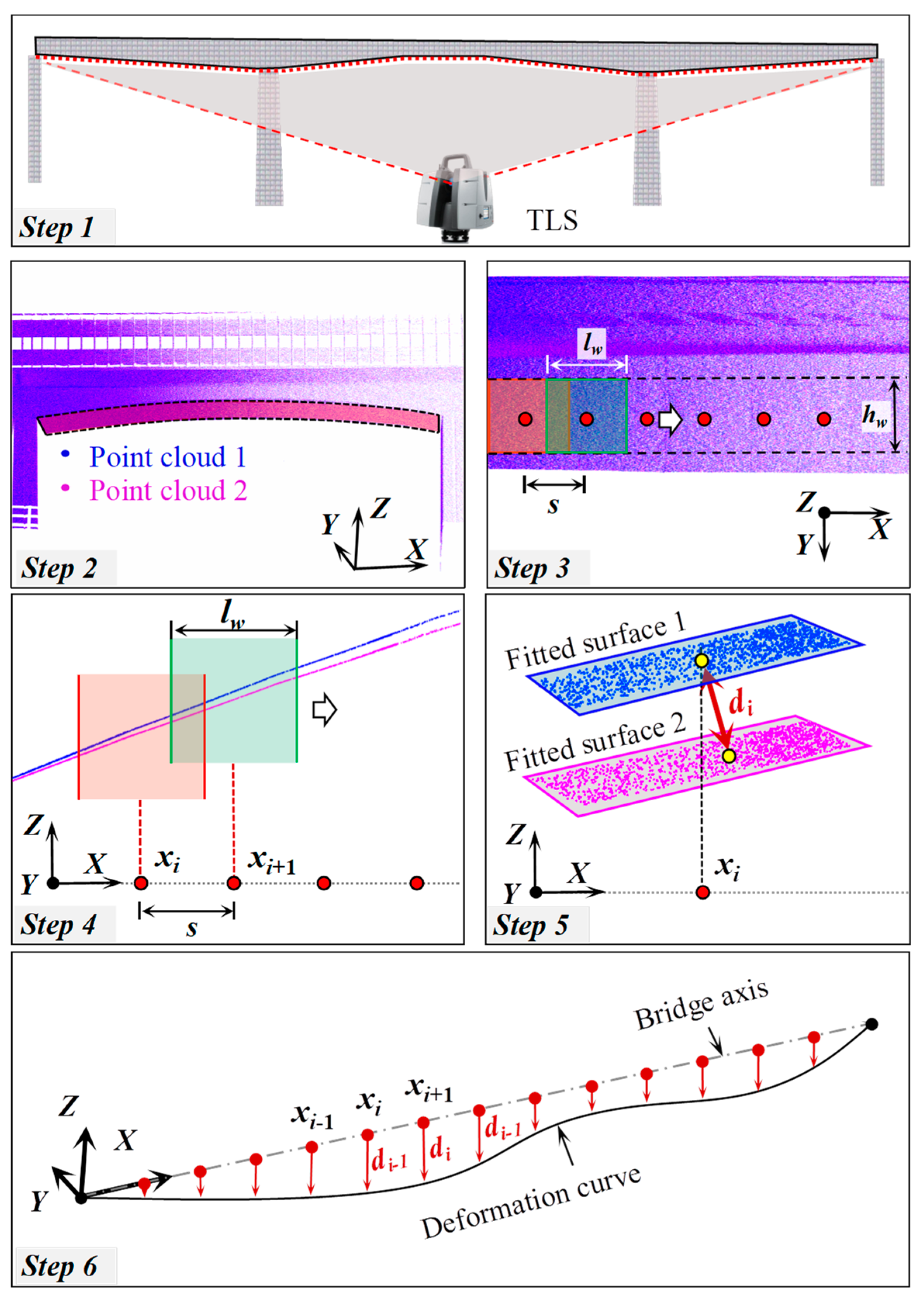
Typically, bridges have beams whose axial length significantly exceeds their cross-sectional dimensions. Consequently, the deformation modes of interest in bridges are usually spatial curves. The X-axis is defined along the spanwise direction of the bridge, the Y-axis along the horizontal direction perpendicular to the spanwise direction, and the Z-axis in the vertical upward direction described as the deformation direction. Deformation due to gravitational effects manifests as a two-dimensional curve in the XZ plane. When factors such as lateral foundation slip and uneven illumination of sunlight are considered, the deformation mode of the bridge becomes a 3D curve. However, this mode can still be decomposed into two-dimensional curves in the XY and XZ planes. Computing the deformation curves in the XY and XZ planes separately from the point cloud can sufficiently capture the spatial deformation mode of a bridge using TLS. The deformation curves in the XY plane are derived from the point clouds at the bottom or top surfaces of the beams, whereas the deformation curves in the XZ plane are computed from the point clouds on the sides of the beams. The general steps of the TLS-based spatial continuous deformation monitoring method for bridges proposed in this study are shown in Figure 1.

Figure 1.
Key steps of bridge deformation mode monitoring method.
The proposed deformation mode calculation method integrates the sliding window and surface fitting methods, and is referred to as the SWSF method. The sliding window is used to separate point cloud blocks with the same boundary from two epoch point clouds. The sliding window method has previously been used for object detection and image filtering [53,54]. The surface function is used to fit the local surface of the bridge corresponding to the two epoch point cloud blocks separately. Due to the noise in the bridge point cloud following a Gaussian distribution, the M-estimation method based on least squares is used for surface fitting. The noise distribution in the bridge point cloud is described in detail in Section 3.2.3. The geometric deviation between the fitted surfaces is considered as the deformation value of the bridge within the sliding window area. By sliding the window, the deformation value at any position on the bridge axis can be obtained. The specific steps of the method are described as follows:
Step 1: TLS is used to scan the bridge in different periods, and the point clouds in different periods are registered in the same coordinate system.
Step 2: The point cloud for the region of interest is truncated from the two-phase point cloud that has been harmonized in the coordinate system. Figure 1 shows the bottom surface of the main girder. Given that the region of interest may be different in each bridge, this step needs to be performed manually in the preprocessing software of the point cloud.
Step 3: A window with a length of lw and a width of hw is constructed. This window slides along the axis of the region of interest. The step size s is the distance between the centers of adjacent windows, which determines the distance between measurement points on the deformation curve.
Step 4: The X-coordinate of the center of the sliding window i, which is defined as the X-coordinate xi of deformation measurement point i, is calculated.
Step 5: A low-order polynomial surface function is used to fit the two point cloud blocks before and after deformation in sliding window i, resulting in two fitted surfaces: Surfaces 1 and 2. The coordinates (xi, zi) at xi on Surface 1 are initially calculated, and the vertical distance di from point (xi, zi) to Surface 2 is calculated. (xi, di) is a measurement point on the bridge deformation curve.
Step 6: The window is moved to the next position, such as xi+1 = xi+s, and Steps 4 and 5 are repeated to obtain the deformation value di+1. (xi+1, di+1) is another measurement point on the bridge deformation curve. By continuously sliding the window to obtain dense measurement points, a deformation curve is formed.
In Step 5, notably, the deformation calculated by the proposed method represents the normal distance between Surfaces 1 and 2, which is suitable for describing the deformation of beams and tower components with constant cross-sections. However, for components with variable cross-sections, an angle exists between the surface’s normal direction and the deformation direction of the component, such as the bottom surface of the main beam shown in Figure 1. When the bridge’s vertical deformation mode needs to be ascertained, the vertical deformation dzi of measurement point i can be calculated using the following formula:
where is the angle between the surface of the bridge at measurement point i and the deformation direction.
The proposed SWSF deformation calculation method belongs to the model reconstruction method. In terms of the precision of surface reconstruction, the SWSF method is between the triangular mesh and NURBS surface methods. The triangular mesh method directly establishes a triangular plane from three adjacent points, and the noise of the point cloud produces significant and random surface reconstruction errors. The NURBS surface method aims to reconstruct continuous and smooth surfaces for the entire point cloud. The reconstruction process is complex, and the surface has many control parameters. The proposed SWSF method uses a sliding window technique to achieve coverage at any position. Within the sliding window range, low-order surface fitting is implemented to reduce the influence of random noise in the point cloud while avoiding overfitting problems and making the algorithm simple.
The TLS-based bridge deformation measurement error accumulates gradually in the above steps, and the final deformation error is influenced by many complex factors, such as point cloud noise, point cloud registration error, and surface fitting error. In addition, the reasonable size of the sliding window in Step 3 and the choice of fitting surface function in Step 5 directly affect the surface fitting error. Therefore, the deformation measurement error based on TLS and SWSF needs to be systematically modeled and analyzed.
3. Error Analysis of Deformation Measurement Based on TLS
3.1. Error Model
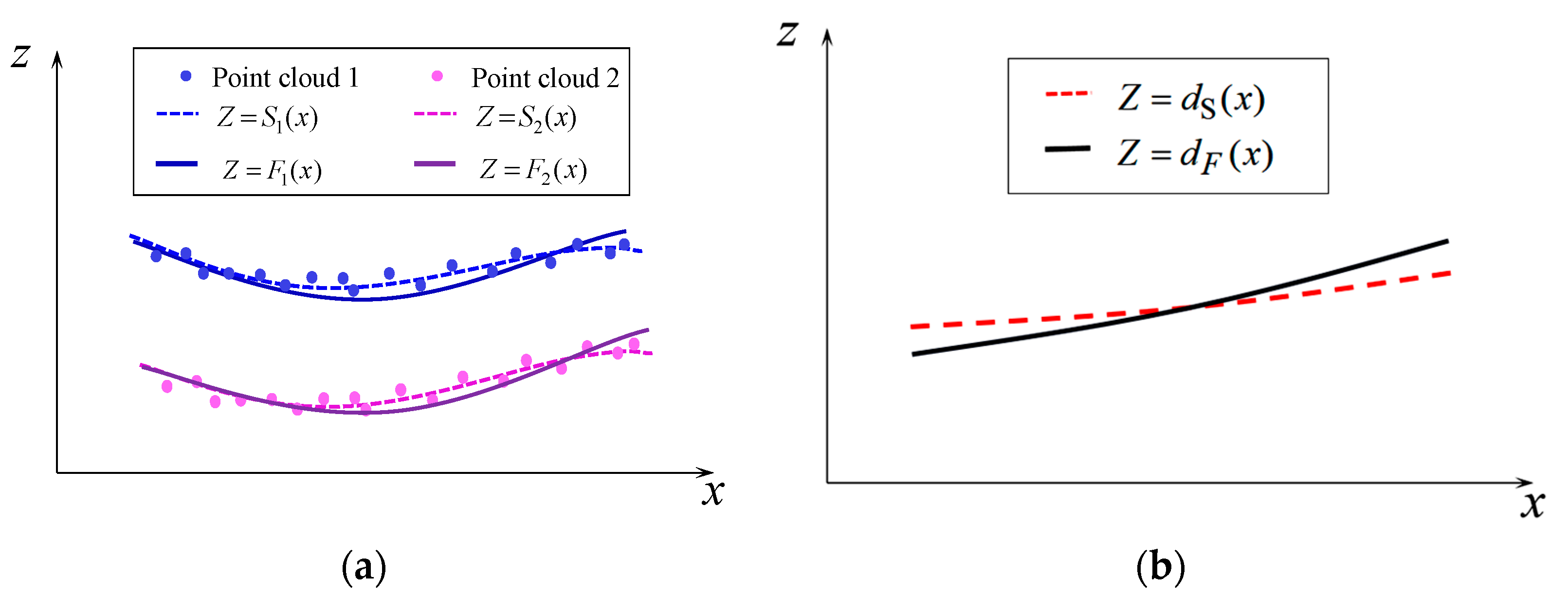
In this study, the point clouds within a sliding window are analyzed, with the pre-deformation point cloud designated as “point cloud 1” and the post-deformation point cloud as “point cloud 2”. Figure 2 illustrates the geometric relationships in the deformation process when utilizing point clouds from a sliding window. Bridge point clouds are typically 3D; however, for a straightforward illustration, Figure 2 restricts its depiction to the functional relationships within the xz plane. In Figure 2a, S1 and S2 represent the actual shape functions of the bridge surface before and after deformation, respectively. Similarly, F1 and F2 denote the fitted shape functions of the bridge surface based on point clouds 1 and 2, respectively. Figure 2b introduces dS as the actual deformation function of the bridge and dF as the calculated deformation function. The method for quantifying deformation is defined as follows:

Figure 2.
Geometric relationships in the deformation process. (a) The shape functions and (b) the deformation function.
The set of point coordinates in point cloud 1 can be defined as a set, which conforms to the following relationship:
where S1(x1i, y1i) is the value of true shape function S1 at (x1i, y1i). Δz1i is the measurement noise of point cloud 1 in the z-direction, which may follow a particular statistical distribution law, such as a Gaussian distribution [55]. {x1i, y1i, z1i} can be considered a superposition of the point sets {x1i, y1i, S1(x1i, y1i)} and {x1i, y1i, Δz1i} in the z-direction. {x1i, y1i, S1(x1i, y1i)} strictly satisfies the actual surface function S1, and {x1i, y1i, Δz1i} is the measurement noise of the point cloud for point cloud 1.
An approximate surface function is utilized to perform surface fitting for point cloud 1, and the resulting fitted surface function is defined as follows:
where F1 consists of two parts: fS1(x, y), which is the fitting function for the set of points {x1i, y1i, S1(x1i, y1i)} following the true shape function S1, and fE1(x, y), which is the fitting function for the measurement noise {x1i, y1i, Δz1i} of the point cloud.
Deformation of the bridge structure owing to damage or external loading occurs, and the true shape function after deformation is as follows:
where dS(x, y) is the actual deformation function of the bridge.
The pseudo-deformation caused by the point cloud registration error is as follows:
The set of point coordinates of point cloud 2 can be considered as {x2j, y2j, z2j}, which satisfies the following relation:
where z2j is divided into four parts: S1(x2j, y2j), dS(x2j, y2j), dR(x2j, y2j), and Δz2j. {x2j, y2j, S1(x2j, y2j)} satisfies the true shape function S1 before deformation, {x2j, y2j, dS(x2j, y2j)} satisfies the true deformation function dS, {x2j, y2j, dR(x2j, y2j)} satisfies the registration error function dR, and {x2j, y2j, Δz2j} is the measurement noise of point cloud 2.
An approximate surface function is employed to conduct surface fitting to point cloud 2, with the corresponding fitted surface function defined as
where F2 consists of four components. fS1*(x, y) is the fitting function of the component matrix {x2j, y2j, S1(x2j, y2j)}. Although {x1i, y1i, S1(x1i, y1i)} and {x2j, y2j, S1(x2j, y2j)} satisfy the shape function S1, their coordinate values are not the same. Therefore, a difference exists in the fitting functions fS1(x, y) and fS1*(x, y). fds(x, y) is the fitting function of the component matrix {x2j, y2j, dS(x2j, y2j)}. fdR(x, y) is the fitting function of the component matrix {x2j, y2j, dR(x2j, y2j)}. fE2(x, y) is the fitting function of the component matrix {x2j, y2j, Δz2j)}.
Subtracting Equation (8) from Equation (4) yields the following computational deformation function of the structure:
By subtracting the actual deformation function from the calculated deformation function (Equation (9)), the error of the deformation measurement is obtained as follows:
where the error of deformation measurement consists of four items: Ed, ES, EN, and ER. Ed is the structural deformation fitting error, which is mainly generated by the inconsistency between the selected fitting function of the point cloud and the actual structural deformation function. The relative fitting error of the surface shape is ES. When the selected fitting function is inconsistent with the actual shape function, the fitting results of the different point clouds (e.g., {x1i, y1i, S1(x1i, y1i)} and {x2j, y2j, S1(x2j, y2j)}) with the same shape function are different; EN is the relative fitting error of the measurement noise ({x1i, y1i, Δz1i)} and {x2j, y2j, Δz2j)}), although {x1i, y1i, Δz1i)} and {x2j, y2j, Δz2j)} may follow the same noise distribution rule. Randomness is observed in the fitting results of the measurement noise components of the point clouds in different periods owing to the randomness of the samples. ER is the fitted value of the registration bias component when the point clouds in two periods are registered to the same coordinate system.
3.2. Error Analysis
3.2.1. Error Ed
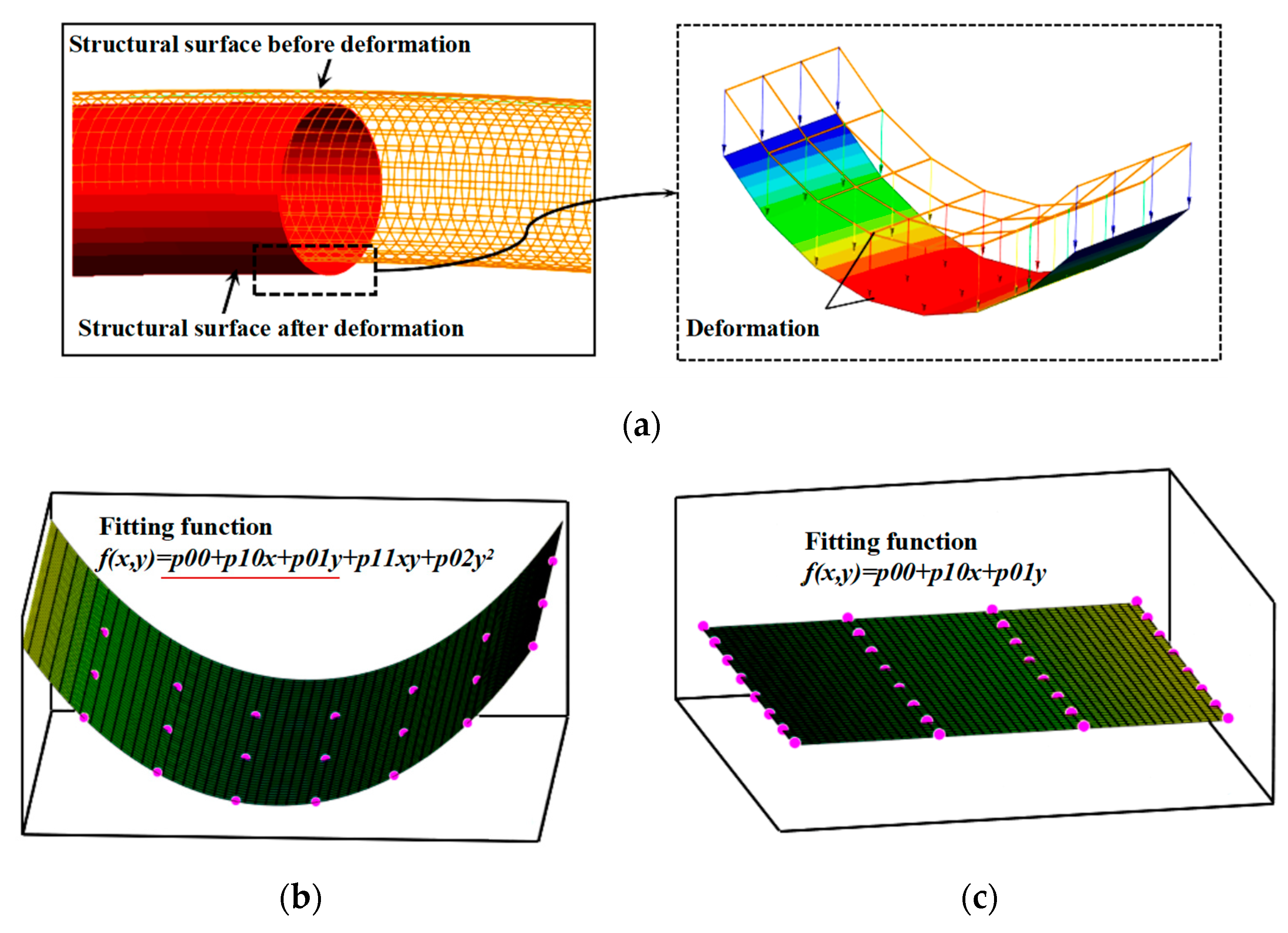
In common bridge structures, the cross-section of components is mainly polygonal and quasi-circular. Therefore, within the sliding window range, the local surface shape of the bridge is a simple plane or curved surface. The first- or second-order fitting function can accurately approximate the local surface shape. In addition, the overall deformation shape of the bridge may be a complex surface function owing to the small range of the sliding window. However, the deformation inside the sliding window can be regarded as a rigid translation of the local surface of the bridge. That is, the deformation function within the sliding window range usually satisfies a first-order plane function. The aforementioned inference is a fundamental characteristic of common bridges, which serves as the basis for analyzing the error Ed in the following text.
Taking bridges with circular cross-sections as the analysis object, we elaborate in detail on the deformation error component Ed. Given that the span of the bridge significantly exceeds its cross-sectional dimensions, its deformation can be conceptualized as an overall translation of the cross-section, as depicted in Figure 3a. A second-order surface function can be used to approximate the shape of the local surface area, as shown in Figure 3b. The deformation shape of the local surface can be accurately fitted with a first-order plane function, as demonstrated in Figure 3c. These fitting results also confirm the correctness of the aforementioned inference. Notably, the higher-order surface function encompasses elements of the first-order surface function. Therefore, when a higher-order surface is used to fit the point cloud of a bridge’s local surface, the deformation function is automatically and precisely included in the surface fitting result. In conclusion, for bridge deformation analysis, the selection of any first-order or higher-order fitting function will not result in a deformation error Ed.

Figure 3.
Relationship between local surface function and local deformation function. (a) Forms of deformation of bridges, (b) local surface fitting, and (c) local deformation fitting.
3.2.2. Error ES
When the chosen fitting function accurately describes the local surface shape of the bridge, the fitting result is accurate, and the error ES is equal to 0. The chosen function is only an approximate fit to the actual shape. Moreover, as long as the input point cloud coordinate matrix changes, the fitting result will also change. In real scanning scenarios, even in the absence of any measurement noise, the point cloud coordinate matrix is not the same for the same area scanned at different times. The reason is that keeping the coordinate system and the starting angle of the two scans exactly the same is difficult. Therefore, deviation exists in the results of the two fits because the positions of the point clouds from the two scans are not the same, and this deviation is the error ES.
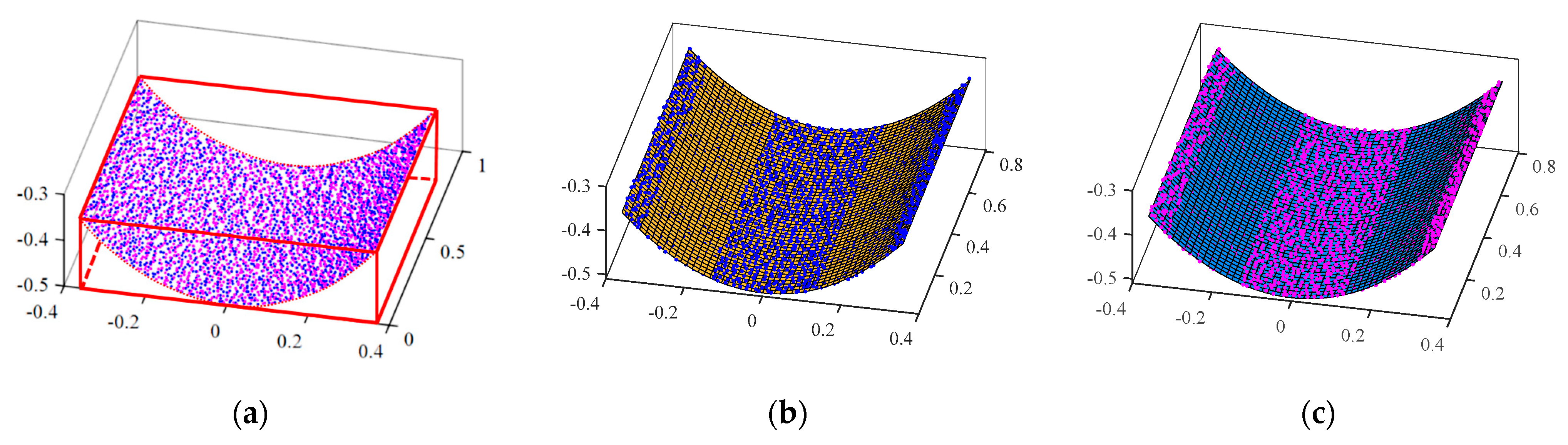
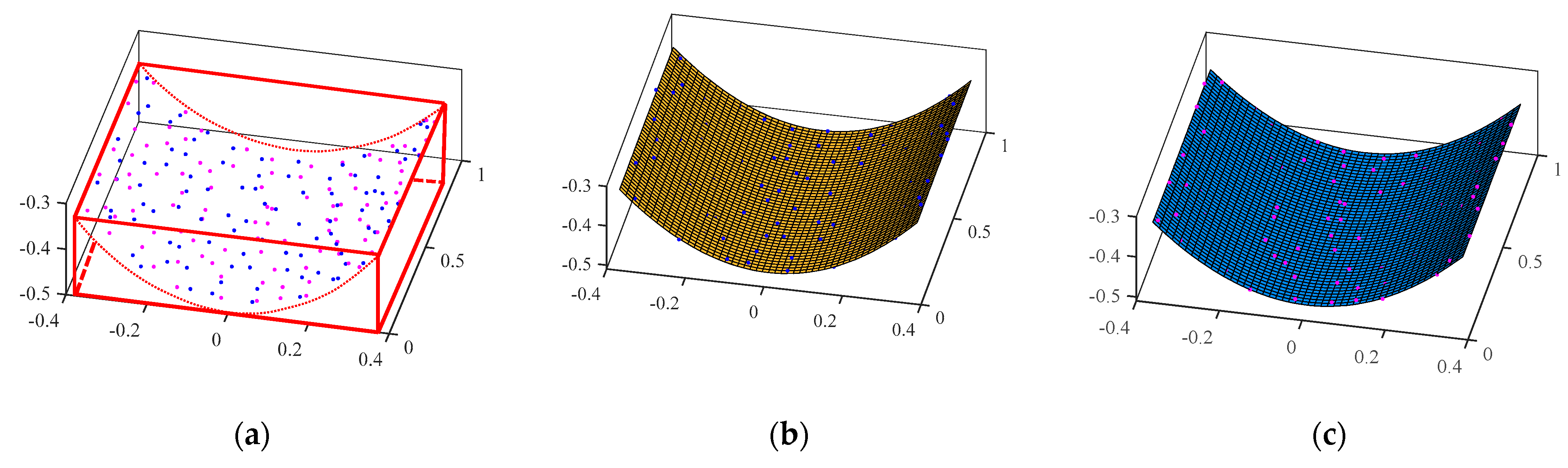
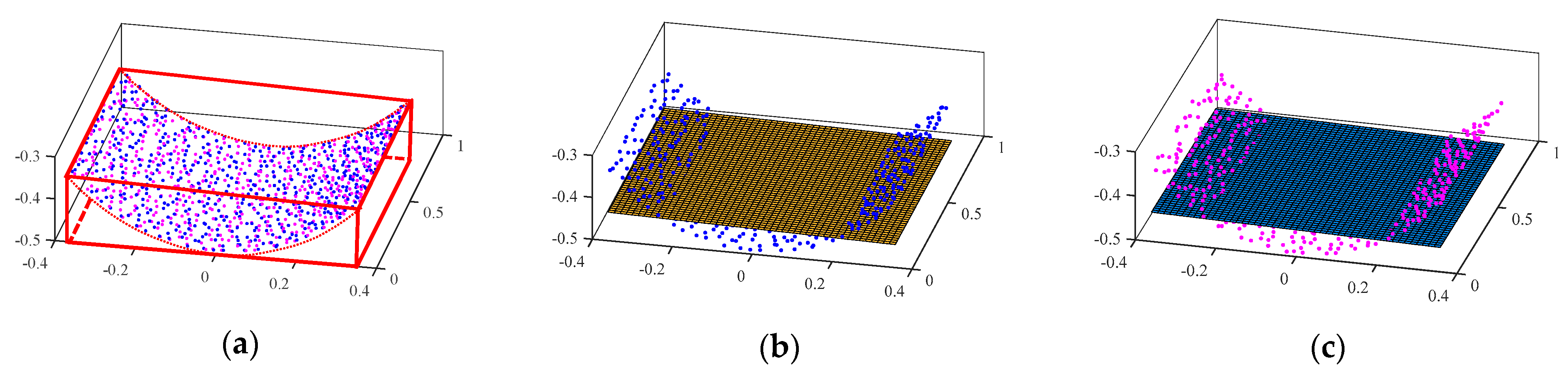
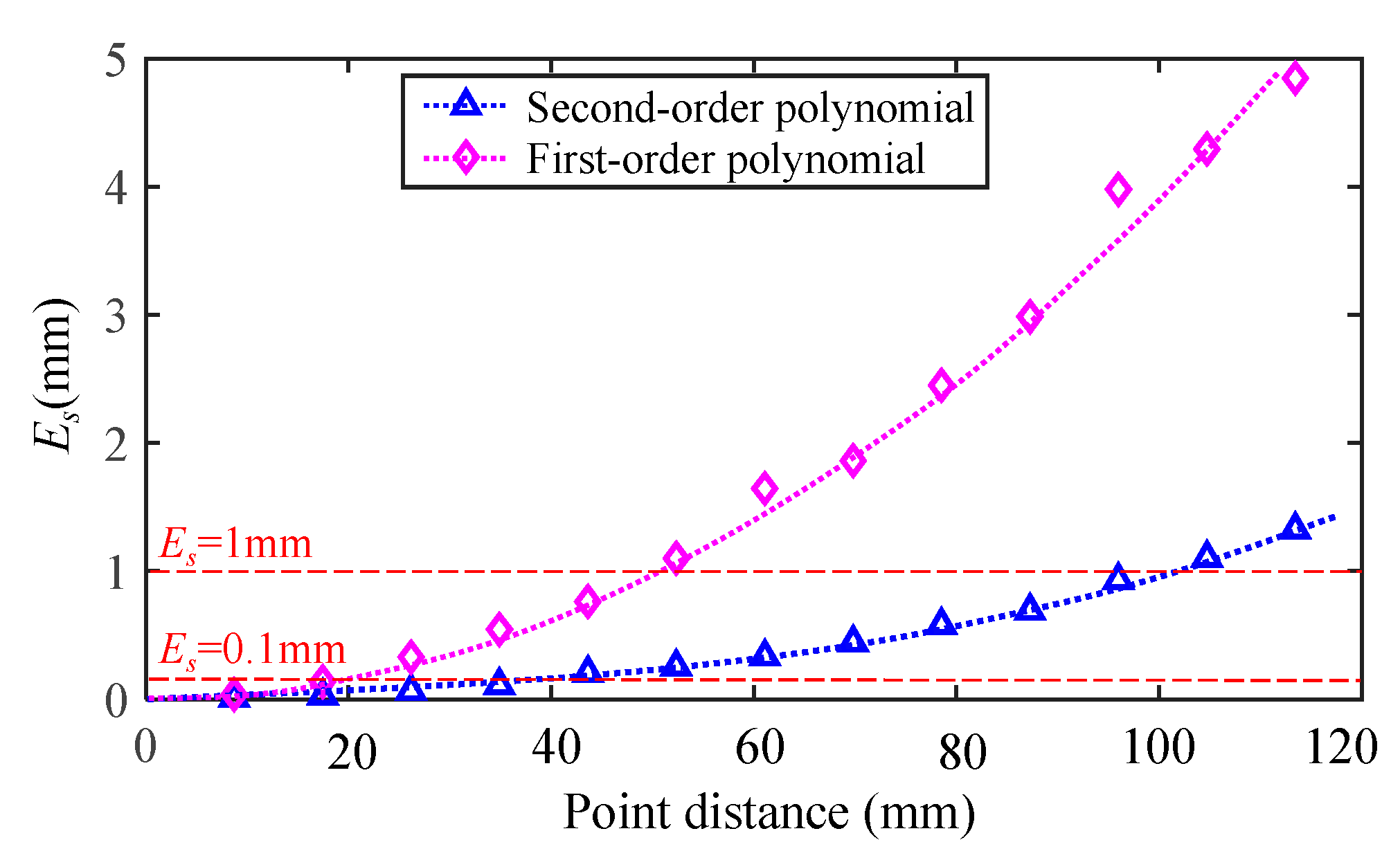
Further study showed that the ES is mainly related to the point distance of the point cloud and the type of fitting function. Manually generating point clouds 1 and 2 is necessary to investigate the characteristics of ES. First, two different point clouds were obtained by performing two random samples on the same surface function, which were free of any measurement noise. Cylinders were used as surface functions for this study. Then, two localized point cloud blocks were truncated from the two generated point clouds using the same sliding window, as shown in Figure 4a. Figure 4, Figure 5 and Figure 6 demonstrate the fitting effects of choosing different fitting functions for different point cloud densities. Figure 4 shows an example of fitting a cylindrical surface point cloud using a second-order surface function in a dense point cloud, whereas Figure 5 shows an example of fitting a second-order surface function in a sparse point cloud scenario. Then, Figure 6 shows an example of fitting a cylindrical surface point cloud using a first-order plane function. Practically, the fitted surfaces in Figure 4, Figure 5 and Figure 6 all deviate from the original point cloud owing to the inconsistency between the chosen fitting function and the actual shape function of the structure. However, in each example, the difference between the fitting results of point clouds 1 and 2, that is, ES, is very small. Figure 7 demonstrates this pattern, showing ES versus the point distance of the point clouds. In the figure, ES is calculated as the maximum gap between the fitted surfaces of point clouds 1 and 2. Given that randomness exists in the location of the point cloud in each scan, the data in Figure 7 show the average value of the results of 1000 previous simulation experiments that were counted. As shown in Figure 7, ES increases nonlinearly with increasing point distance. Hence, the following quantitative conclusions can be drawn. For the first-order planar function, ES is less than 0.1 mm when the point spacing is less than 20 mm, and less than 1 mm when the point distance is less than 50 mm. For the second-order surface function, ES is less than 0.1 mm when the point distance is less than 40 mm, and less than 1 mm when the point distance is less than 100 mm. Therefore, in a dense point cloud environment where the point spacing is less than 20 mm, ES can be kept at 0.1 mm even if a planar function with a large difference from the actual shape is used as the fitting function. The point distance can be increased from 20 mm to 40 mm while keeping ES at 0.1 mm by increasing the order of the fitting function from the first to the second order, which means that the effective scanning distance can be increased by a factor of 2. Taking the Leica P50 scanner as an example, its finest scanning mode has point spacing of 0.8 mm at a distance of 10 m [35]. The maximum allowable range when keeping ES at 0.1 mm is up to 500 m. The smaller the size of the sliding window, the simpler the local surface shape it captures, and the more accurate the fitting results are. In the case shown in Figure 7, with unfavorable considerations, the center angle of the circle corresponding to the range extracted by the sliding window reaches 60°. In this extreme situation, ES can still easily remain within 0.1 mm. Therefore, ES is negligible in a general bridge scenario.

Figure 4.
Dense point cloud high-order polynomial fitting surface. (a) Sliding window range, (b) point cloud 1, and (c) point cloud 2.

Figure 5.
Sparse point cloud high-order polynomial fitting surface. (a) Sliding window range, (b) point cloud 1, and (c) point cloud 2.

Figure 6.
First-order polynomial fitting surface results. (a) Sliding window range, (b) point cloud 1, and (c) point cloud 2.

Figure 7.
Error Es.
3.2.3. Error EN
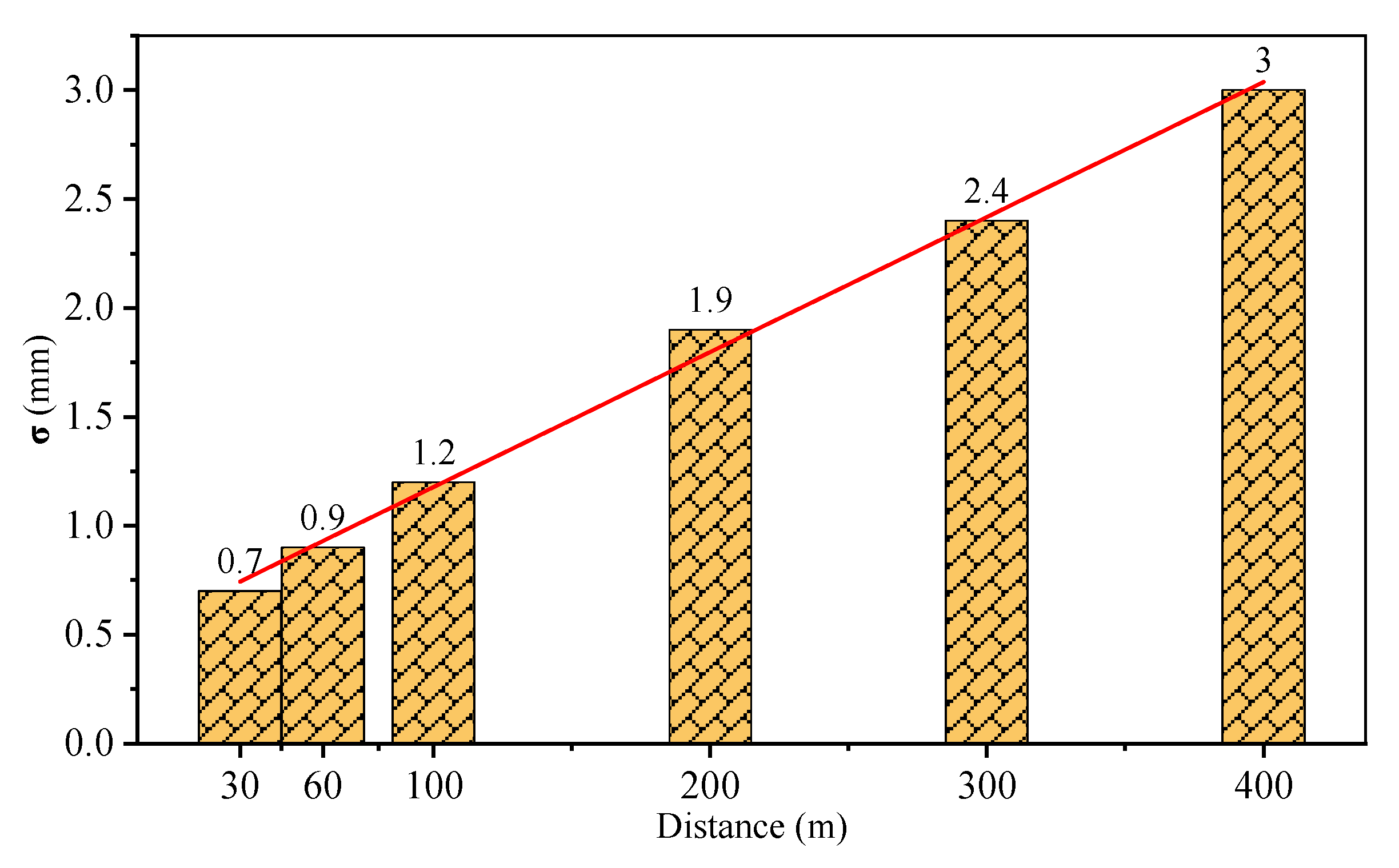
The measurement noise of a scanner can be considered to satisfy a Gaussian distribution [55]. To further study the relationship between scanning point cloud noise and range, a point cloud noise survey experiment was conducted using a Leica P50 scanner. The experiment was conducted in an open square with set ranging distances of 30, 60, 100, 200, 300, and 400 m. The probability density of point cloud noise was statistically analyzed. The point cloud noise in all six tests met the Gaussian distribution . Figure 8 shows the variation in the standard deviation of the measured point cloud noise with the range. Overall, the measured values of showed a linear relationship with the range. When the range was 100 m, was 1.2 mm; when the range was 400 m, was 3.0 mm. For every 100 m increase in range, the average increase in was 0.6 mm.

Figure 8.
Relationship between the standard deviation of point cloud noise and range.
Considering that the scanning measurement noise satisfies the Gaussian distribution (N~(0, σ2)), {x1i, y1i, Δz1i} and {x2j, y2j, Δz2j} are planar point clouds with Gaussian fluctuations near the plane of z = 0. According to Equation (9), EN denotes the geometric difference between the fitted plane of the measurement noise {x1i, y1i, Δz1i} and that of the measurement noise {x2j, y2j, Δz2j}. Therefore, EN can be equated to the difference between the mean values of {Δz2j} and {Δz1i}.
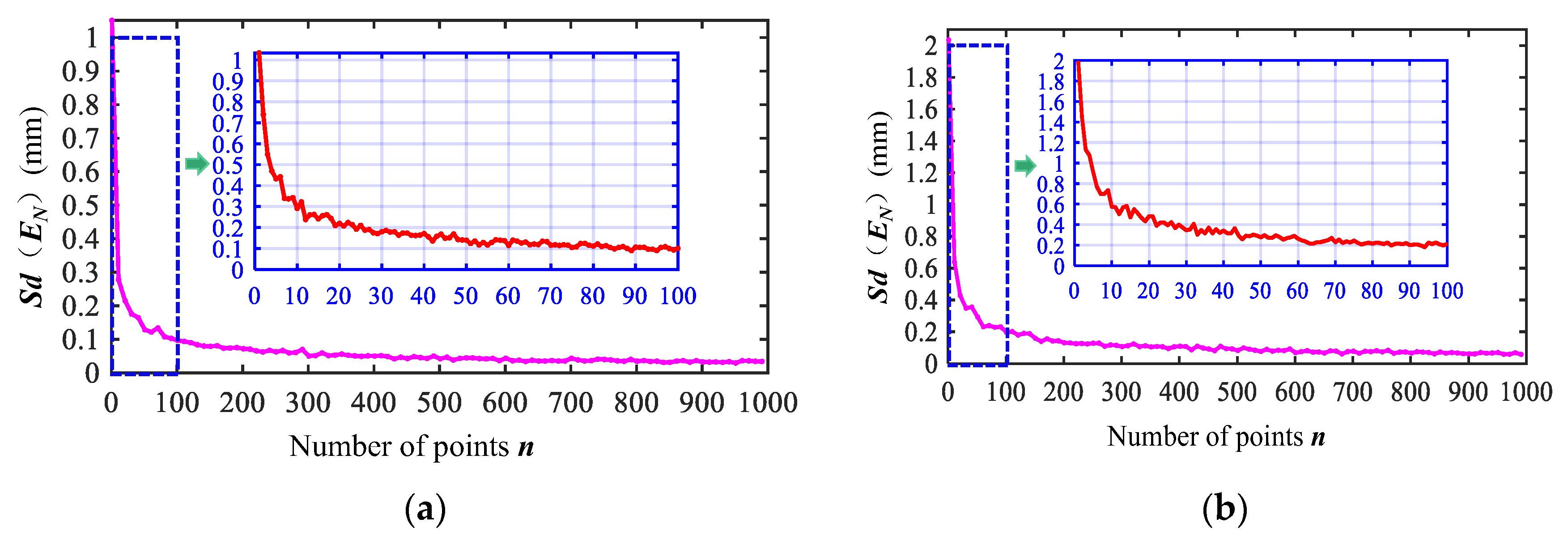
Clearly, EN exhibits random variability and is significantly influenced by the number of points n involved in the computation and the noise standard deviation σ. This study conducted extensive numerical simulation experiments to explore the probabilistic statistical relationship between EN, n, and σ. Figure 9 shows the results. Given that EN is a random term, it cannot be directly quantified. The standard deviation of EN obtained from multiple simulation experiments is defined as Sd(EN). Sd(EN) is used to describe EN. In this study, each Sd(EN) was statistically obtained from the results of 1000 random experiments. Figure 9a demonstrates the trend in Sd(EN) as the number of samples n increases at σ = 1 mm. Similarly, Figure 9b shows the trend in Sd(EN) with an increasing number of samples n at σ = 2 mm. The data indicate that Sd(EN) decreases rapidly and then stabilizes as the number of points n involved in the calculation increases. Comparing Figure 9a and b, the variation pattern of Sd(EN) with n is completely the same. Therefore, the variation in the standard deviation of point cloud noise will not change the variation pattern of Sd(EN) and n. When the number of points used in the calculation reaches approximately 100, EN reduces to one-tenth of the noise standard deviation level. Additionally, a point cloud with σ = 2 mm requires at least 100 points, whereas a point cloud with σ = 2 mm necessitates a minimum of 500 points to maintain Sd(EN) within 0.1 mm.

Figure 9.
Relationship between Sd(EN) and number of points n. (a) σ = 1 mm and (b) σ = 2 mm.
Figure 10a depicts the relationship between Sd(EN) and the number of points n and the noise standard deviation σ within the range of 0.5–3 mm. Overall, when the number of points n is fixed, Sd(EN) exhibits a linear relationship with σ. Twice the value of Sd(EN) is adopted as the characterization value of EN to further quantify the numerical magnitude of EN. According to the basic characteristics of Gaussian distribution, this characterization value can achieve a reliability of 95%, which meets the general requirements of engineering measurement. When Sd(EN) = 0.05 mm, the characterization error of EN is 0.1 mm, and the relationship between the number of points n and noise σ is shown in Figure 10b. When the point cloud noise σ = 1, 2, and 3 mm, the sliding window point cloud needs at least 400, 1600, and 3500 points, respectively. When Sd(EN) = 0.5 mm, the characterization error of EN is 1 mm, and the relationship between the number of points n and noise σ is shown in Figure 10c. When the point cloud noise σ = 1, 2, and 3 mm, the sliding window point cloud needs at least 6, 17, and 38 points, respectively.

Figure 10.
Regularity diagram of EN. (a) EN versus the number of points n and noise σ, (b) relationship between the number of points n and noise σ when Sd(EN) = 0.05 mm, and (c) relationship between the number of points n and noise σ when Sd(EN) = 0.5 mm.
In summary, the error EN is a random term that is significantly related to the noise of the point cloud and the number of points in the sliding window point cloud. Overall, when the standard deviation of the point cloud noise is in the range of 0–3 mm, to make the error EN less than 0.1 mm, the number of points n in the sliding window point cloud should be greater than 300. To make the error EN less than 1 mm, the number of points n in the sliding window point cloud should be greater than 38. The number of points n in the sliding window point cloud is related to the size of the sliding window and the density of the point cloud. n can be calculated according to the following formula:
where d is the point spacing of the sliding window point cloud, which is related to the resolution setting mode of the scanner.
Therefore, in the SWSF method proposed in Section 2, the size of the sliding window mainly depends on the number of points in the sliding window. The width hw of the sliding window is the width of the deformation-concerned region, and it is recommended that the maximum value is used as much as possible. In the example shown in Figure 1, the sliding window width hw can be equal to the width of the bottom surface of the main beam. On the basis of the determined minimum number of points n in the sliding window, the point spacing d, and the sliding window width hw, the length lw of the sliding window can be calculated using Equation (10).
3.2.4. Error ER
Deformation monitoring can be divided into two types: continuous and periodic measurements. In continuous measurement scenarios, which typically require a short interval between two deformation measurements, a scanning method with a fixed instrument position is employed, eliminating the registration error associated with two-phase point clouds. For periodic observations, however, the instrumentation often needs to be reset, necessitating multiple point cloud registrations into a consistent coordinate system. This case requires the use of precise registration methods to ensure minimal registration error. The iterative closest point (ICP) method and its variants are currently widely used, but they are all data-driven approaches, which are not suitable in the presence of deformations [56]. The black and white targets and spherical targets developed by the Leica High-definition Surveying (HDS) system are currently the most commonly used target-based registration methods. According to the user manual of the Leica scanning system, the registration error of HDS targets can reach the millimeter level. Recently, Zhou et al. introduced a registration method based on triangular pyramid targets [34]. The experimental results of this study indicate that the accuracy of triangular pyramid registration surpasses that of ICP and spherical markers, with registration errors ranging between 0.2 and 0.8 mm. Therefore, for continuous and periodic monitoring, the deformation monitoring error of the proposed method framework can reach the submillimeter level.
3.2.5. Summary of Measurement Errors
For the proposed method of bridge deformation monitoring, when deformation is calculated within a sliding window using fitting plane or surface subtraction methods, the components of the deformation measurement error include three parts: error ES, error EN, and error ER. Error ES arises from the discrepancy between the chosen fitting function and the actual surface function of the bridge. This error can be maintained within 0.1 mm in a suitable point cloud density environment (point spacing < 40 mm). Error EN is primarily induced by scanning point cloud noise and varies with the point cloud noise and the number of points in the sliding window. Error ER is largely dependent on the point cloud registration method and can currently reach submillimeter levels. In summary, the proposed deformation measurement method has been demonstrated to achieve submillimeter accuracy. In continuous monitoring scenarios without registration errors, the monitoring error of the bridge deformation mode based on TLS and SWSF mainly originates from EN. Therefore, by reasonably setting the size of the sliding window, the number of points within the sliding window can meet the requirements of the corresponding monitoring accuracy level, and the deformation measurement accuracy can reach the level of 0.1 mm. Table 1 shows the summary of each error.

Table 1.
Error summary table.
4. Precision Verification Experiment
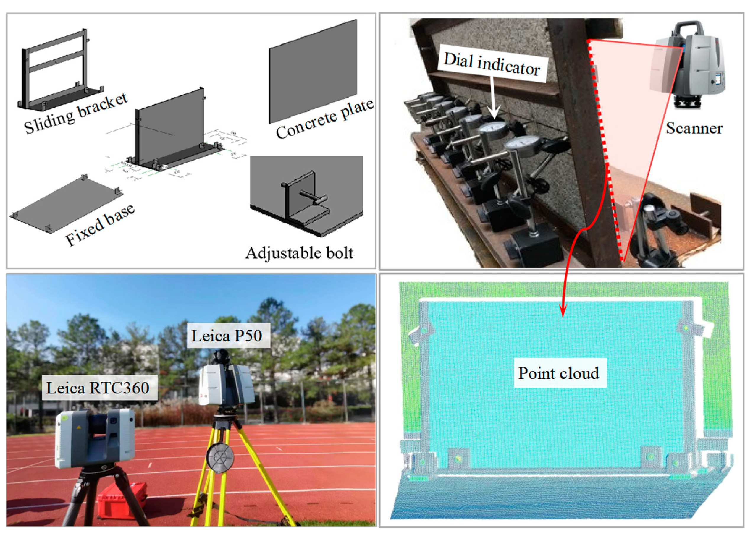
To verify the submillimeter accuracy level of deformation monitoring based on TLS and SWSF, a high-precision experimental device was designed, as shown in Figure 11. The experimental device is mainly composed of a fixed base, a sliding bracket, a concrete plate, and an adjustable bolt. The concrete plate is poured using steel formwork commonly used in practical bridges. Therefore, the concrete plate is similar to the local surface of the real bridge. The concrete plate is used to simulate the bridge surface within the sliding window region in the SWSF method. The size of the concrete plate is 0.6 m × 0.4 m. The fixed base is fixed on the ground and kept strictly motionless during the experiment. The sliding bracket is bound to the concrete plate and placed on the base surface. The movement of the sliding support is controlled by fine-tuning the bolts on the base plate to simulate the small deformation of the bridge. Multiple dial gauges are placed behind the concrete slab to measure accurately its true deformation value. The Leica P50 scanner is used in the experiment. Two scanners with different accuracy levels are used, Leica P50 and Leica RTC360.
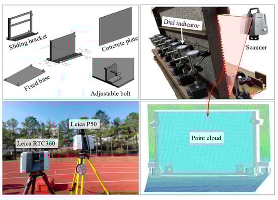
Figure 11.
Deformation accuracy verification experiment.
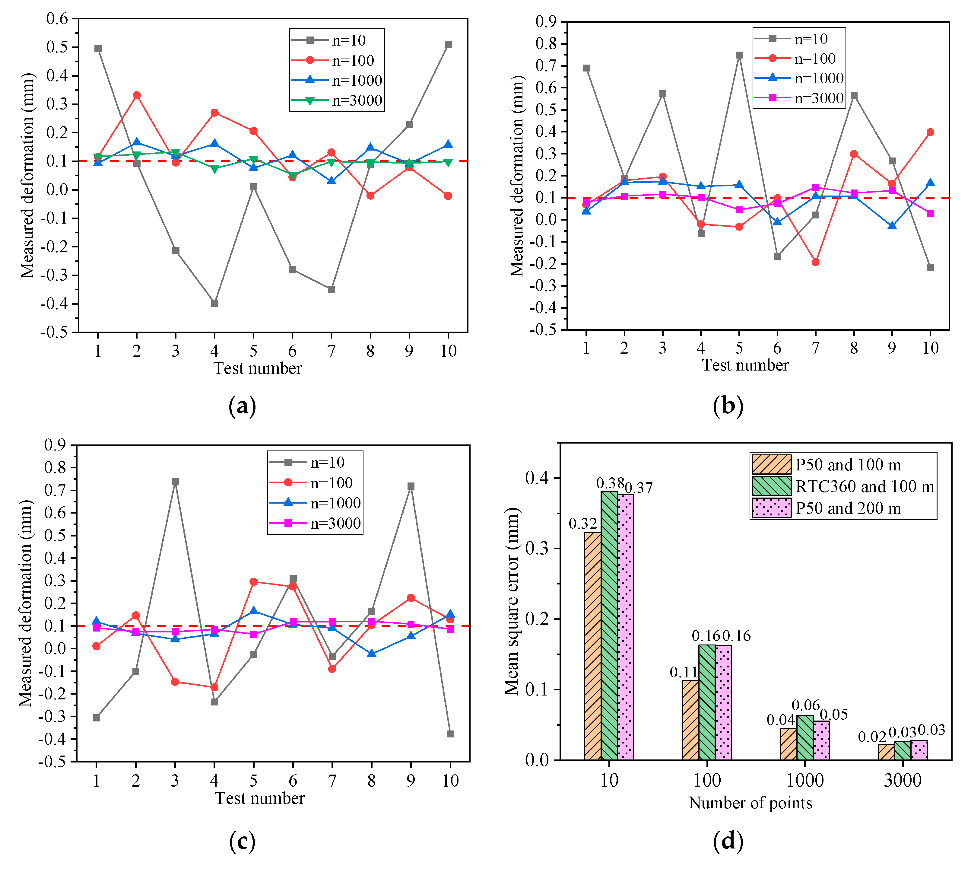
The experiment involved conducting 10 scanning tests in 100 m and 200 m ranging conditions. Since the maximum range of Leica RTC360 is 130 m, Leica RTC360 was only used to conduct the tests with a 100 m range. By fine-tuning the bolts, the concrete plate was deformed by 0.1 mm relative to its initial position. During the experiment, the position of the scanner remained unchanged. Therefore, no registration error existed. The scanning points on the concrete plate in each test are not fewer than 3000 points. When a scan cannot obtain enough points, the scan must be repeated to increase the number of points on the concrete plate. By sampling the point cloud of the concrete slab to simulate the point clouds with different numbers of points in the sliding window, the calculation of deformation in the sliding window used a first-order function fitting. The details of the experimental scheme are shown in Table 2. The experimental results are shown in Figure 12. The deformation calculation results for different ranges and scanners are shown in Figure 12a–c. The mean square error of 10 deformation tests is shown in Figure 12d. Figure 12a–c indicate that the deformation calculation results tend to be stable with the increase in the number of points in the sliding window. The change in range and the difference in scanners did not affect the experimental results. When the number of points was 10, the deformation calculation results fluctuated significantly and could not effectively identify the 0.1 mm deformation. When the number of points was above 1000, the deformation calculation results stabilized around 0.1 mm and effectively identified the 0.1 mm deformation. Figure 12d indicates that the mean square error of the deformation test results decreases significantly with the increase in the number of points in the sliding window. This result was consistent for different ranges and different scanners. In addition, when the numbers of points in the sliding window were 10 and 100, the mean square error was affected by the noise standard deviation of the point cloud. The standard deviation of point cloud noise was 1.2 mm at 100 m range for the scanner Leica P50, 2.0 mm at 100 m range for the scanner Leica RTC360, and 1.9 mm at 200 m range for the scanner Leica P50. When the standard deviation of point cloud noise was larger, the mean square error of the deformation test results was relatively larger. However, when the number of points in the sliding window exceeded 1000, the mean square error of the deformation test results was less than 0.1 mm, and the point cloud noise was not sensitive to the mean square error of the deformation test results. The experimental results show that the measurement accuracy of deformation mode monitoring based on TLS and SWSF can be improved by increasing the number of points in the sliding window. This result is consistent with the simulation results shown in Figure 10. At the same time, under the condition of a range of 200 m, the deformation monitoring error based on TLS and SWSF can be measured to be less than 0.1 mm.
Table 2.
Overview of experimental scheme.

Figure 12.
Deformation monitoring results under different conditions: (a) Leica P50 and range of 100 m, (b) Leica RTC360 and range of 100 m, (c) Leica P50 and range of 200 m, and (d) mean square error of deformation monitoring error.
5. Real Bridge Testing
5.1. Introduction to Bridge
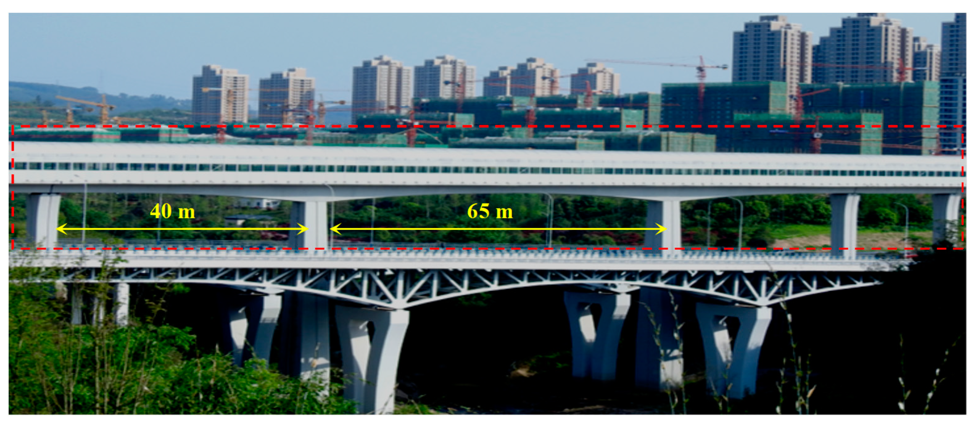
Figure 13 shows a continuous rigid-frame bridge in Chongqing, China, spanning 40 m + 65 m + 40 m. This test bridge is nearing completion and will soon be open to traffic. Prior to its official operation, the bridge must undergo a load test to verify if its static and dynamic characteristics align with expectations. Deformation is a critical indicator of the static properties of a bridge. However, given that this bridge is a highly rigid rail bridge, the expected deformation under the test load is only a few millimeters, necessitating deformation monitoring with submillimeter accuracy. The bridge’s main girder surface is enclosed by a sound barrier, making the use of a precision level impractical. Additionally, with a clearance of 50 m beneath the main girder, the use of dial indicators is not feasible owing to the lack of support. Therefore, a high-precision, noncontact method for deformation monitoring is necessary.

Figure 13.
Site plan of a rail bridge.
5.2. Test Scheme
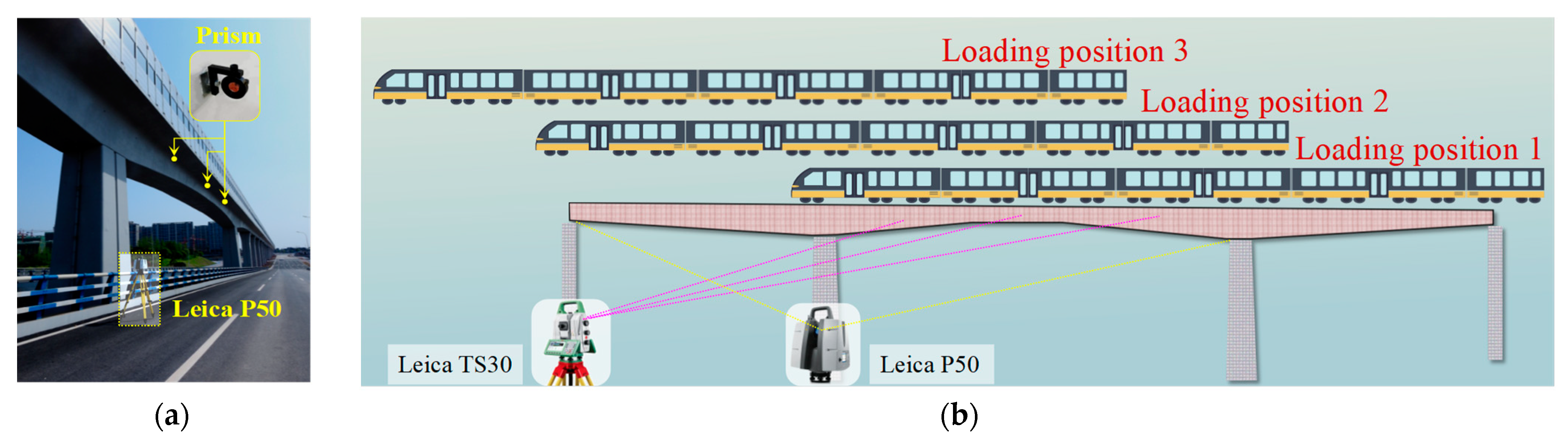
The proposed method was implemented in the deformation monitoring of the load tests of this bridge. At the same time, the traditional monitoring method of total station and prism combination, which is the most commonly used method in bridge monitoring, was adopted in parallel. Three prisms were installed on the side of the main girder using a lift truck positioned at L/4, L/2, and 3L/4 of the bridge’s midspan. The scanner used was a Leica P50, set up beside the pier of the midspan of the test bridge, allowing complete observation of the left side- and center-span areas. A scanning resolution of 3.1 mm @10 m was used, and the single measurement time was approximately 3 min. The distance between the farthest point of the midspan and the scanner was 65 m, and the corresponding noise standard deviation of the point cloud was about 1 mm. The total station used was Leica TS30, which was set up next to the pier of the side span. The distance between the farthest prism and the total station was 85 m. The automatic prism identification accuracy of the Leica TS30 was 1 mm. In terms of single-point measurement accuracy, the selected Leica P50 and Leica TS30 had comparable accuracy. The layout plan of measuring instruments and loading trains is shown in Figure 14. The scanner and total station maintained their positions throughout the test, indicating that the error ER described in Section 3.2 did not exist. The load was applied using a fully loaded train stationed at three preset loading positions. Given the varying positions of the train load, different deformations were induced on the test bridge.

Figure 14.
Test scheme. (a) Instrument and (b) loading scheme for trains.
5.3. Test Results
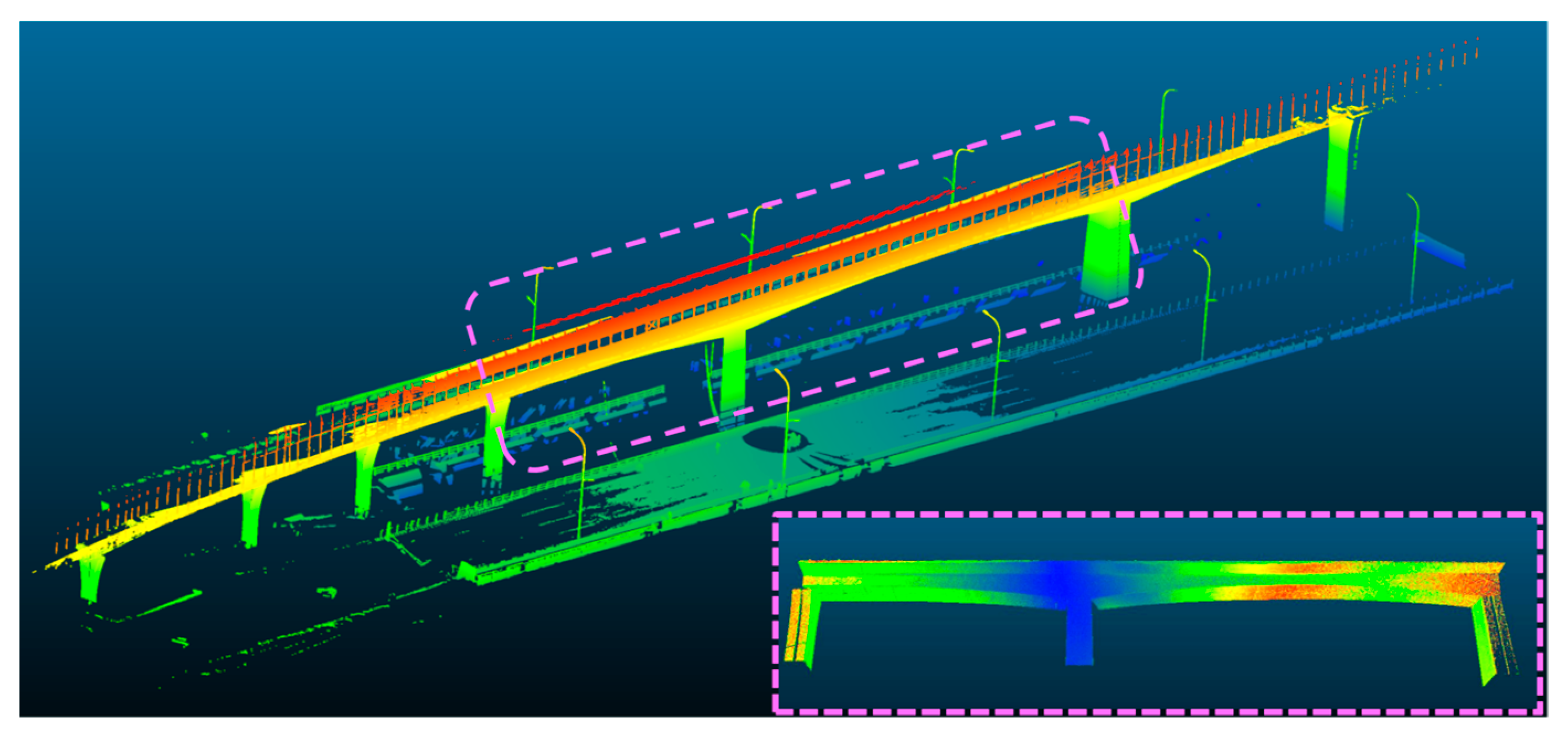
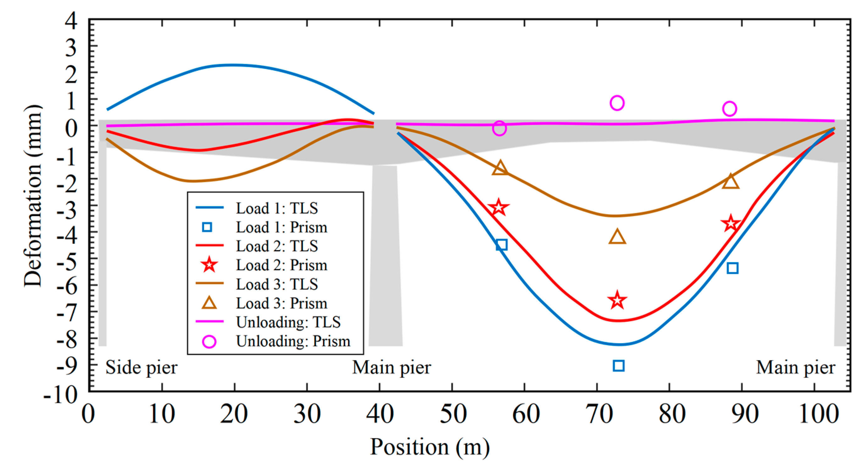
Figure 15 presents the point cloud model of the test bridge. The point clouds of the bottom surfaces of the left side span and the center span were completely captured. A total of five sets of data were collected throughout the testing process, including the initial state, three loading states, and the state after unloading. The point cloud of the bridge bottom surface was used to calculate the deformation. In the calculation process using the proposed method, the sliding window width was set to 3 m and the length to 1 m. The numbers of points in the sliding window on the left and farthest sides of the midspan were 120,000 and 2500, respectively. According to the numerical simulation results in Figure 10b and the experimental results in Figure 12d, under the conditions of a point cloud noise standard deviation of 1 mm and a sliding window point count of 2500, the deformation calculation accuracy of the sliding window could reach 0.1 mm. The average number of points in the point cloud within the sliding window was 8000. The step distance for sliding windows was 0.2 m. Figure 16 shows the results of the deformation test. The results include deformations after three loading states and after unloading. The test results demonstrate that the proposed SWSF method successfully captures the deformation modes of the side and center spans of the test bridge. The deformation curves were extremely smooth without fluctuating noise, indicating the strong robustness of the SWSF method in real bridge environments. This result indicates that the proposed method is robust indoors and outdoors. When comparing the test results of the proposed method with those of the prisms, the deformation results of the prisms fluctuate around the deformation curves obtained by the proposed method, with a maximum positive deviation of 1.1 mm and a maximum negative deviation of −1.0 mm. Given that the total station monitors bridge deformation by monitoring the changes in the prism, the automatic prism identification error is the main source of error in deformation monitoring. The automatic prism identification error of the Leica TS30 was 1 mm, which is consistent with the fluctuation in the measured data. Furthermore, the unloading deformation test results of the proposed method are analyzed. The unloading deformation is the difference between the state data when the train completely exits the bridge and the unloaded initial state data. Given that the test bridge is newly constructed, it should have no damage under normal conditions. Thus, the bridge is in the elastic phase with loading within the design’s allowable range, and the theoretical deformation after unloading is 0 mm. The unloaded deformations in the side- and center-span regions obtained using the proposed method were close to 0 mm, with a maximum residual deformation of 0.2 mm. The residual deformation values of the three measuring points of the total station were −0.3, 0.9, and 0.6 mm. Clearly, the residual deformation indirectly proves that the proposed method accurately captures the deformation modes of the bridge. The monitoring results of the deformation mode also demonstrate the absence of initial structural damage in this test bridge.

Figure 15.
Point cloud model of the test bridge.
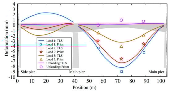
Figure 16.
Results for the test bridge.
The practical application results show that the proposed method is a noncontact, high-precision monitoring technique that does not require the presetting of any reflective markers. The method can accomplish comprehensive coverage data collection within the visible range in just a few minutes. In comparison with the commonly used total station method, the proposed method improves the deformation monitoring accuracy from the millimeter level to the submillimeter level and transforms the discrete measurement point data format into a spatially continuous deformation mode.
6. Conclusions
In this study, a high-precision deformation monitoring method for bridges based on TLS is introduced. The contributions of this research are significant in two main aspects: (1) the establishment of a TLS-based method for calculating deformation modes of bridges, characterized by its substantial noise-resistant capability; and (2) the development of a scanning point cloud-based deformation measurement error model that is applicable for general bridges, accompanied by a quantitative analysis of each error component. The research and experimental verification presented in this study lead to the following conclusions:
- The proposed bridge deformation monitoring method based on TLS and SWSF can obtain spatially continuous and smooth deformation curves of bridges. The fitting of point clouds within the sliding window only requires the use of first- or second-order polynomial functions.
- The deformation measurement method, which is based on the differential of the fitted shape of sliding window point clouds, mainly comprises four components of error. These components are associated with the choice of fitting function, the density of the point cloud, the noise within the point cloud, and the accuracy of point cloud registration. Among these, the errors that cannot be neglected are those caused by the noise in the point cloud and the registration error.
- The deformation measurement error caused by point cloud noise is related to the noise level and the number of points in the sliding window. At a certain level of point cloud noise, the deformation calculation error can be reduced to the submillimeter level, up to 0.1 mm, by simply increasing the number of points in the sliding windows. This conclusion was verified in experiments with ranges of 100 m and 200 m.
- In comparison with the total station method, the proposed method does not require the preinstallation of reflective targets or sensors, and it has the advantages of high accuracy, no contact, high efficiency, and wide monitoring range. These advantages were verified in a real bridge test. The proposed method is also applicable to structures with simple surface geometries, such as buildings and dams.
In this study, registration error was eliminated by keeping the scanner’s position constant, making the method ideal for scenarios where the instrument is permanently fixed or in short-term monitoring. In periodic monitoring scenarios where the scanner needs to be moved, reducing the registration error of two-phase point clouds remains a significant research focus. In addition, for flexible bridges in operation, structural vibrations owing to external excitation, which will appear as a significant point cloud noise, cannot be ignored. Developing strategies to eliminate these vibration noises is crucial for extending the applicability of the proposed method to flexible bridges.
Author Contributions
Methodology: Y.Z., J.Z. and J.X.; software: G.H. and L.Z.; validation: J.Y. and H.Z.; writing—original draft preparation: Y.Z., J.Z. and G.H.; writing—review and editing: Y.Z., J.X. and J.Y.; visualization: H.Z. and L.Z.; funding acquisition: J.X. All authors have read and agreed to the published version of the manuscript.
Funding
This research is funded by the ChongQing Postdoctoral Science Foundation (CSTB2022NSCQ-BHX0741), ChongQing Science Fund for Distinguished Young Scholars (CSTB2023NSCQ-JQX0029), Chongqing Natural Science Foundation of China (CSTB2022TIAD-KPX0205), and Science and Technology Project of Sichuan Provincial Transportation Department (2023-ZL-03).
Data Availability Statement
Data are contained within the article.
Conflicts of Interest
The authors declare no conflicts of interest.
References
- Feng, D.; Feng, M.Q. Model Updating of Railway Bridge Using In Situ Dynamic Displacement Measurement under Trainloads. J. Bridge Eng. 2015, 20, 04015019. [Google Scholar] [CrossRef]
- Moreu, F.; Jo, H.; Li, J.; Kim, R.E.; Cho, S.; Kimmle, A.; Scola, S.; Le, H.; Spencer, B.F.; LaFave, J.M. Dynamic Assessment of Timber Railroad Bridges Using Displacements. J. Bridge Eng. 2015, 20, 04014114. [Google Scholar] [CrossRef]
- Feng, D.; Feng, M.Q. Output-only damage detection using vehicle-induced displacement response and mode shape curvature index. Struct. Control Health Monit. 2016, 23, 1088–1107. [Google Scholar] [CrossRef]
- Tang, Q.; Xin, J.; Jiang, Y.; Zhang, H.; Zhou, J. Dynamic Response Recovery of Damaged Structures Using Residual Learning Enhanced Fully Convolutional Network. 2024. Available online: https://www.worldscientific.com/doi/10.1142/S0219455425500087 (accessed on 16 June 2024).
- Sarthak, J.; Shrikant Madhav, H. Linear Variable Differential Transducer (LVDT) & Its Applications in Civil Engineering. Int. J. Transp. Eng. Technol. 2017, 3, 62–66. [Google Scholar] [CrossRef]
- Liu, Y.; Deng, Y.; Cai, C.S. Deflection monitoring and assessment for a suspension bridge using a connected pipe system: A case study in China. Struct. Control Health Monit. 2015, 22, 1408–1425. [Google Scholar] [CrossRef]
- Zhu, S.F.; Zhou, Z.X.; Wu, H.J. Application of semi-closed connected pipe differential pressure sensor in bridge deflection measurement. Transducer Microsyst. Technol. 2014, 33, 150–153. [Google Scholar]
- Yu, J.; Meng, X.; Yan, B.; Xu, B.; Fan, Q.; Xie, Y. Global Navigation Satellite System-based positioning technology for structural health monitoring: A review. Struct. Control Health Monit. 2020, 27, e2467. [Google Scholar] [CrossRef]
- Moschas, F.; Stiros, S. Measurement of the dynamic displacements and of the modal frequencies of a short-span pedestrian bridge using GPS and an accelerometer. Eng. Struct. 2011, 33, 10–17. [Google Scholar] [CrossRef]
- Vazquez, B.G.E.; Gaxiola-Camacho, J.R.; Bennett, R.; Guzman-Acevedo, G.M.; Gaxiola-Camacho, I.E. Structural evaluation of dynamic and semi-static displacements of the Juarez Bridge using GPS technology. Measurement 2017, 110, 146–153. [Google Scholar] [CrossRef]
- Zhao, L.; Yang, Y.; Xiang, Z.; Zhang, S.; Li, X.; Wang, X.; Ma, X.; Hu, C.; Pan, J.; Zhou, Y.; et al. A Novel Low-Cost GNSS Solution for the Real-Time Deformation Monitoring of Cable Saddle Pushing: A Case Study of Guojiatuo Suspension Bridge. Remote Sens. 2022, 14, 5174. [Google Scholar] [CrossRef]
- Lee, H.S.; Hong, Y.H.; Park, H.W. Design of an FIR filter for the displacement reconstruction using measured acceleration in low-frequency dominant structures. Int. J. Numer. Methods Eng. 2010, 82, 403–434. [Google Scholar] [CrossRef]
- Kim, K.; Choi, J.; Koo, G.; Sohn, H. Dynamic displacement estimation by fusing biased high-sampling rate acceleration and low-sampling rate displacement measurements using two-stage Kalman estimator. Smart Struct. Syst. 2016, 17, 647–667. [Google Scholar] [CrossRef]
- Kim, J.; Kim, K.; Sohn, H. Autonomous dynamic displacement estimation from data fusion of acceleration and intermittent displacement measurements. Mech. Syst. Signal Process. 2014, 42, 194–205. [Google Scholar] [CrossRef]
- Wang, Z.-C.; Geng, D.; Ren, W.-X.; Liu, H.-T. Strain modes based dynamic displacement estimation of beam structures with strain sensors. Smart Mater. Struct. 2014, 23, 125045. [Google Scholar] [CrossRef]
- Shen, S.; Wu, Z.; Yang, C.; Wan, C.; Tang, Y.; Wu, G. An Improved Conjugated Beam Method for Deformation Monitoring with a Distributed Sensitive Fiber Optic Sensor. Struct. Health Monit. 2010, 9, 361–378. [Google Scholar] [CrossRef]
- Ma, Z.; Chung, J.; Liu, P.; Sohn, H. Bridge displacement estimation by fusing accelerometer and strain gauge measurements. Struct. Control Health Monit. 2021, 28, e2733. [Google Scholar] [CrossRef]
- Ehrhart, M.; Lienhart, W. Accurate measurements with image-assisted total stations and their prerequisites. J. Surv. Eng. 2017, 143, 04016024. [Google Scholar] [CrossRef]
- Kohut, P.; Holak, K.; Uhl, T.; Ortyl, Ł.; Owerko, T.; Kuras, P.; Kocierz, R. Monitoring of a civil structure’s state based on noncontact measurements. Struct. Health Monit. 2013, 12, 411–429. [Google Scholar] [CrossRef]
- Xu, Y.; Brownjohn, J.; Kong, D. A non-contact vision-based system for multipoint displacement monitoring in a cable-stayed footbridge. Struct. Control Health Monit. 2018, 25, e2155. [Google Scholar] [CrossRef]
- Yoon, H.; Shin, J.; Spencer, B.F., Jr. Structural Displacement Measurement Using an Unmanned Aerial System. Comput.-Aided Civ. Infrastruct. Eng. 2018, 33, 183–192. [Google Scholar] [CrossRef]
- Mathew, M.; Ellenberg, A.; Esola, S.; McCarthy, M.; Bartoli, I.; Kontsos, A. Multiscale deformation measurements using multispectral optical metrology. Struct. Control Health Monit. 2018, 25, e2166. [Google Scholar] [CrossRef]
- Wu, T.; Tang, L.; Zhang, X.; Liu, Y.; Li, X.; Zhou, Z. An Improved Structural Displacement Monitoring Approach by Acceleration-Aided Tilt Camera Measurement. Struct. Control Health Monit. 2023, 2023, 6247516. [Google Scholar] [CrossRef]
- Jiang, S.; Zhang, J.; Gao, C. Bridge Deformation Measurement Using Unmanned Aerial Dual Camera and Learning-Based Tracking Method. Struct. Control Health Monit. 2023, 2023, 4752072. [Google Scholar] [CrossRef]
- Shao, S.; Zhou, Z.; Deng, G.; Du, P.; Jian, C.; Yu, Z. Experiment of Structural Geometric Morphology Monitoring for Bridges Using Holographic Visual Sensor. Sensors 2020, 20, 1187. [Google Scholar] [CrossRef] [PubMed]
- Deng, G.; Zhou, Z.; Shao, S.; Chu, X.; Jian, C. A Novel Dense Full-Field Displacement Monitoring Method Based on Image Sequences and Optical Flow Algorithm. Appl. Sci. 2020, 10, 2118. [Google Scholar] [CrossRef]
- Aryan, A.; Bosché, F.; Tang, P. Planning for terrestrial laser scanning in construction: A review. Autom. Constr. 2021, 125, 103551. [Google Scholar] [CrossRef]
- El-Omari, S.; Moselhi, O. Integrating 3D laser scanning and photogrammetry for progress measurement of construction work. Autom. Constr. 2008, 18, 1–9. [Google Scholar] [CrossRef]
- Tang, P.; Huber, D.; Akinci, B.; Lipman, R.; Lytle, A. Automatic reconstruction of as-built building information models from laser-scanned point clouds: A review of related techniques. Autom. Constr. 2010, 19, 829–843. [Google Scholar] [CrossRef]
- Qin, G.; Zhou, Y.; Hu, K.; Han, D.; Ying, C. Automated Reconstruction of Parametric BIM for Bridge Based on Terrestrial Laser Scanning Data. Adv. Civ. Eng. 2021, 2021, 8899323. [Google Scholar] [CrossRef]
- Yang, L.; Cheng, J.C.P.; Wang, Q. Semi-automated generation of parametric BIM for steel structures based on terrestrial laser scanning data. Autom. Constr. 2020, 112, 103037. [Google Scholar] [CrossRef]
- Kim, M.-K.; Wang, Q.; Park, J.-W.; Cheng, J.C.P.; Sohn, H.; Chang, C.-C. Automated dimensional quality assurance of full-scale precast concrete elements using laser scanning and BIM. Autom. Constr. 2016, 72, 102–114. [Google Scholar] [CrossRef]
- Kim, D.; Kwak, Y.; Sohn, H. Accelerated cable-stayed bridge construction using terrestrial laser scanning. Autom. Constr. 2020, 117, 103269. [Google Scholar] [CrossRef]
- Zhou, Y.; Han, D.; Hu, K.; Qin, G.; Xiang, Z.; Ying, C.; Lidu, Z.; Hu, X. Accurate Virtual Trial Assembly Method of Prefabricated Steel Components Using Terrestrial Laser Scanning. Adv. Civ. Eng. 2021, 2021, 9916859. [Google Scholar] [CrossRef]
- Park, H.S.; Lee, H.M.; Adeli, H.; Lee, I. A New Approach for Health Monitoring of Structures: Terrestrial Laser Scanning. Comput.-Aided Civ. Infrastruct. Eng. 2007, 22, 19–30. [Google Scholar] [CrossRef]
- Mosalam, K.M.; Takhirov, S.M.; Park, S. Applications of laser scanning to structures in laboratory tests and field surveys. Struct. Control Health Monit. 2014, 21, 115–134. [Google Scholar] [CrossRef]
- Sánchez-Rodríguez, A.; Riveiro, B.; Conde, B.; Soilán, M. Detection of structural faults in piers of masonry arch bridges through automated processing of laser scanning data. Struct. Control Health Monit. 2018, 25, e2126. [Google Scholar] [CrossRef]
- Zhou, Y.; Xiang, Z.; Zhang, X.; Wang, Y.; Han, D.; Ying, C. Mechanical state inversion method for structural performance evaluation of existing suspension bridges using 3D laser scanning. Comput.-Aided Civ. Infrastruct. Eng. 2022, 37, 650–665. [Google Scholar] [CrossRef]
- Liang, D.; Zhang, Z.-S.; Sui, C.-L.; Pu, J.; Su, L.-C.; Zhao, K. Performance assessment of self-anchored suspension footbridge using 3D laser scanning. Struct. Control Health Monit. 2022, 29, e2978. [Google Scholar] [CrossRef]
- Lõhmus, H.; Ellmann, A.; Märdla, S.; Idnurm, S. Terrestrial laser scanning for the monitoring of bridge load tests—Two case studies. Surv. Rev. 2017, 50, 270–284. [Google Scholar] [CrossRef]
- Soni, A.; Robson, S.; Gleeson, B. Structural monitoring for the rail industry using conventional survey, laser scanning and photogrammetry. Appl. Geomat. 2015, 7, 123–138. [Google Scholar] [CrossRef]
- Truong-Hong, L.; Laefer, D.F. Using Terrestrial Laser Scanning for Dynamic Bridge Deflection Measurement. 2014. Available online: http://hdl.handle.net/10197/7495 (accessed on 13 August 2014).
- Shen, N.; Wang, B.; Ma, H.; Zhao, X.; Zhou, Y.; Zhang, Z.; Xu, J. A review of terrestrial laser scanning (TLS)-based technologies for deformation monitoring in engineering. Measurement 2023, 223, 113684. [Google Scholar] [CrossRef]
- Girardeau-Montaut, D.; Roux, M.; Marc, R.; Thibault, G. Change detection on point cloud data acquired with a ground laser scanner. Int. Arch. Photogramm. Remote Sens. Spat. Inf. Sci. 2005, 36, W19. [Google Scholar]
- Yu, Y.; Guan, H.; Li, D.; Jin, S.; Chen, T.; Wang, C.; Li, J. 3-D Feature Matching for Point Cloud Object Extraction. IEEE Geosci. Remote Sens. Lett. 2020, 17, 322–326. [Google Scholar] [CrossRef]
- Si, H.; Wei, X. Feature extraction and representation learning of 3D point cloud data. Image Vis. Comput. 2024, 142, 104890. [Google Scholar] [CrossRef]
- Meneses Diego, M.; Zheng, L.; Guo, Q. Identification and Quantification of Surface Depressions on Grassy Land Surfaces of Different Topographic Attributes Using High-Resolution Terrestrial Laser Scanning Point Cloud and Triangulated Irregular Network. J. Hydrol. Eng. 2023, 28, 04023004. [Google Scholar] [CrossRef]
- Khameneifar, F.; Feng, H.-Y. Establishing a balanced neighborhood of discrete points for local quadric surface fitting. Comput.-Aided Des. 2017, 84, 25–38. [Google Scholar] [CrossRef]
- Dimitrov, A.; Gu, R.; Golparvar-Fard, M. Non-Uniform B-Spline Surface Fitting from Unordered 3D Point Clouds for As-Built Modeling. Comput.-Aided Civ. Infrastruct. Eng. 2016, 31, 483–498. [Google Scholar] [CrossRef]
- Dąbrowski, P.; Zienkiewicz, M. Impact of cross-section centers estimation on the accuracy of the point cloud spatial expansion using robust M-estimation and Monte Carlo simulation. Measurement 2022, 189, 110436. [Google Scholar] [CrossRef]
- Janicka, J.; Rapiński, J.; Błaszczak-Bąk, W.; Suchocki, C. Application of the Msplit estimation method in the detection and dimensioning of the displacement of adjacent planes. Remote Sens. 2020, 12, 3203. [Google Scholar] [CrossRef]
- Duchnowski, R.; Wyszkowska, P. Msplit Estimation Approach to Modeling Vertical Terrain Displacement from TLS Data Disturbed by Outliers. Remote Sens. 2022, 14, 5620. [Google Scholar] [CrossRef]
- Dong, Q.; Wang, S.; Chen, X.; Jiang, W.; Li, R.; Gu, X. Pavement crack detection based on point cloud data and data fusion. Philos. Trans. R. Soc. A 2023, 381, 20220165. [Google Scholar] [CrossRef]
- Gao, R.; Park, J.; Hu, X.; Yang, S.; Cho, K. Reflective Noise Filtering of Large-Scale Point Cloud Using Multi-Position LiDAR Sensing Data. Remote Sens. 2021, 13, 3058. [Google Scholar] [CrossRef]
- Zahs, V.; Winiwarter, L.; Anders, K.; Williams, J.G.; Rutzinger, M.; Höfle, B. Correspondence-driven plane-based M3C2 for lower uncertainty in 3D topographic change quantification. ISPRS J. Photogramm. Remote Sens. 2022, 183, 541–559. [Google Scholar] [CrossRef]
- Zhao, X.; Kargoll, B.; Omidalizarandi, M.; Xu, X.; Alkhatib, H. Model Selection for Parametric Surfaces Approximating 3D Point Clouds for Deformation Analysis. Remote Sens. 2018, 10, 634. [Google Scholar] [CrossRef]

Disclaimer/Publisher’s Note: The statements, opinions and data contained in all publications are solely those of the individual author(s) and contributor(s) and not of MDPI and/or the editor(s). MDPI and/or the editor(s) disclaim responsibility for any injury to people or property resulting from any ideas, methods, instructions or products referred to in the content. |
© 2024 by the authors. Licensee MDPI, Basel, Switzerland. This article is an open access article distributed under the terms and conditions of the Creative Commons Attribution (CC BY) license (https://creativecommons.org/licenses/by/4.0/).