Abstract
This work focuses on investigating the accuracy of 3D reconstructions from fixed stereo-photogrammetric monitoring systems through different camera calibration procedures. New reliable and effective calibration methodologies that require minimal effort and resources are presented. A full-format camera equipped with fixed 50 and 85 mm focal length optics is considered, but the methodologies are general and can be applied to other systems. Four different calibration strategies are considered: (i) full-field calibration (FF); (ii) multi-image on-the-job calibration (MI); (iii) point cloud-based calibration (PC); and (iv) self (on-the-job) calibration (SC). To evaluate the calibration strategies and assess their actual performance and practicality, two test sites are used. The full-field calibration, while very reliable, demands significant effort if it needs to be repeated. The multi-image strategy emerges as a favourable compromise, offering good results with minimal effort for its realisation. The point cloud-based method stands out as the optimal choice, balancing ease of implementation with quality results; however, it requires a reference 3D point cloud model. On-the-job calibration with monitoring images is the simplest but least reliable option, prone to uncertainty and potential inaccuracies, and should hence be avoided. Ultimately, prioritising result reliability over absolute accuracy is paramount in continuous monitoring systems.
1. Introduction
Over the last twenty years, there has been a progressive use of photogrammetric techniques to support monitoring activities across a wide range of applications, such as environmental [1,2,3], architectural, mechanical or structural [4,5,6,7], and many others [8]. The affordability of hardware and operational costs, along with the simplicity of components and their high scalability, have made photogrammetric systems exceptionally well-suited for activities that require enduring or frequent acquisitions. For this purpose, the deployment of fixed on-site installed systems (sometimes referred to as time-lapse photogrammetric systems), consisting of a series of fixed acquisition stations that allow continuous monitoring [9,10,11,12], in some cases in near real-time [13] and in extreme lighting conditions [14,15], has been recorded in recent years. Although such systems exhibit some challenges in providing reliable, precise data over time, they also offer advantages in serviceability and costs that have raised interest in both research and industry applications. One of the first examples of a fixed terrestrial photogrammetric monitoring system can be found in [16]. The authors tested a stereo camera system on the Mont de la Saxe (Italy) landslide and compared its results with much more expensive and complex GbInSAR (Ground-based Interferometric Synthetic Aperture Radar). Similarly, in [17], the authors proposed a framework for generating sequences of Digital Elevation Models (DEMs) to analyse active lava flows using oblique stereo-pair time-lapse imagery. In both contributions, the advantages of fixed camera systems over other monitoring solutions (mainly laser-based or radar-based) were highlighted. These include low equipment cost, high portability, and the potential for greater spatial and temporal scalability. Nevertheless, these systems also require additional investigations to ensure the stability of the camera positions over time, to limit the influence of external causes on the optical characteristics of the acquisition system, and to develop novel methodologies to correct, or account for, such variations during the system’s lifetime.
Ensuring the stability of the reference system is a critical aspect of any monitoring system. Traditional optical geodetic measurements rely on precise centring devices and stable reference points for orientation — a requirement that also applies to laser scanning. However, photogrammetry typically relies on Ground Control Points (GCPs) for georeferencing, since GNSS (Global Navigation Satellite System)- and INS (Inertial Navigation System)-assisted orientation procedures are generally not sufficiently accurate for close-range monitoring purposes. Unfortunately, the collection and image identification of GCPs are time-consuming and costly activities that generally require considerable manual intervention by a human operator, with substantial economic impact on any project application. This problem was highlighted in [18], where a five-camera system was designed for rock slope hazard monitoring and an automated workflow for photogrammetric point cloud registration with a reference TLS (Terrestrial Laser Scanner)-acquired three-dimensional (3D) model (i.e., without the use of GCPs) was presented.
At the same time, camera calibration plays a critical role in ensuring optimal accuracies in these kinds of applications. Consumer-grade digital cameras, especially when subjected to weather events and used over an extended period of time, tend not to guarantee sufficient optical stability [19] over time, the parameters defining the geometric model of the camera (the most commonly used in photogrammetry is the one proposed in [20]) tend to change, and repeatable calibration procedures at regular intervals are required to achieve optimal accuracy. It should be noted that, generally, a fixed photogrammetric monitoring system is comprised of just a few acquisition stations (i.e., cameras) and, consequently, the image block geometry is rather unstable if accurate camera model parameters (i.e., a pre-calibrated fixed camera model) are not considered: not accounting for strong exterior and interior parameters’ correlation could result in poor monitoring performance if the photogrammetric 3D model results are deformed and the repeatability between consecutive periods is compromised. Due to these latter image block geometry weaknesses, estimating the camera model parameters (i.e., performing a camera calibration procedure) on-the-job might lead to inaccurate and strongly parameter-correlated results, as clearly emphasized by all previously cited research studies.
In [21], the effect of poor calibration on the final products and the impact of repeating camera calibration procedures was investigated, and a new approach not requiring periodic re-calibration of the system was presented. In [22], a set of procedures for camera model and system calibration and photogrammetric ground control of the monitoring system was also proposed with the aim of limiting on-site surveying operations and, in particular, limiting the number of GCPs required for proper image orientation and georeferencing.
This work focuses on investigating the performances, in terms of final 3D reconstruction accuracy, of different camera model calibration procedures to be implemented in fixed photogrammetric monitoring systems. A stereo-photogrammetric (i.e., with two cameras) system similar to the one presented in [10] is considered. The practicality of performing these procedures within minimal time requirements in the field (and consequently the reduction of costs) combined with ensuring reliable accuracy of results plays a crucial role in their effective application in real-world monitoring scenarios. Periodic activities for checking and updating the calibration and system orientation parameters need also be considered during the period of system deployment. This study presents the development of new reliable and effective calibration methodologies that require minimal effort and resources to address the practical limitations of standard calibration procedures.
2. Materials and Methods
2.1. Fixed Photogrammetric Monitoring Equipment
The autonomous terrestrial stereo-pair photogrammetric monitoring system developed in [10] was used for the experimental investigation. It comprises two stand-alone units designed to detect volumes falling from sub-vertical rock faces, particularly in surface mining environments. Each unit is housed within an IP67 weatherproof box, ensuring protection from environmental elements, and includes essential components such as a digital single-lens reflex (DSLR) camera, a single-board microprocessor, and an uninterruptible power supply (UPS). The camera utilized is a full-format Nikon D850, boasting a resolution of 45.4 megapixels, that can be equipped with fixed 50 mm focal length optics (AF-S Nikkor 50 mm f/1.8 G Lens) or fixed 85 mm optics (AF-S Nikkor 85 mm f/1.8 G Lens). Integrated with the DSLR camera is a Raspberry Pi 3 Model B (RPi3B) single-board computer, serving as the control hub for acquisition parameters. The RPi3B features an integrated wireless LAN (WLAN) module, enabling seamless connectivity to an external Wi-Fi network for remote control and monitoring. Each unit is powered by a 60 W solar panel and a pair of 26 Ah batteries stored within an IP66 enclosure box. Mounted on the exterior of the camera box is a 5/8” prism mounting screw, which facilitates the temporary installation of a survey prism or GNSS receiver for precise spatial referencing. Moreover, recent redesign efforts by [23] have enhanced the system’s versatility and adaptability. These improvements include provisions for easy installation in diverse locations, adjustable camera box setups to accommodate tilt and rotation for site-specific fields of view, compatibility with different lenses, optimization of the circular sealed aperture, and the incorporation of a shading screen (see Figure 1).
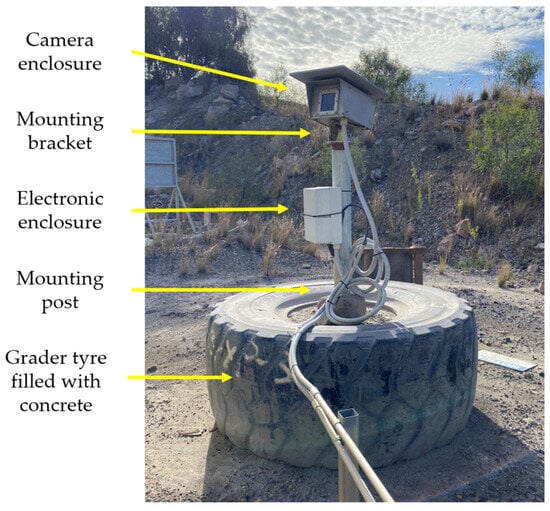
Figure 1.
Picture of the whole re-designed system as installed at a mine site.
2.2. Calibration Procedures
Camera calibration in photogrammetry refers to the process of determining the geometric behaviour of the optical system of a camera, which is essential for accurately back-projecting 3D spatial information from images. Camera calibration can be performed either in a laboratory setting or, as is often the case with off-the-shelf and consumer-grade cameras, through analytical procedures. In the latter case, the process typically involves capturing images of a calibration target (which can be the object to survey itself, in which case the calibration procedure is often referred to as on-the-job [24]) with known geometric properties (e.g., providing a set of GCPs) from various orientations and distances. Then, a specific parametric camera model (e.g., the Brown–Conrady model [20]) is considered to analytically approximate the behaviour of the projective system. The parameters of such a model, referred to as intrinsic parameters, are estimated with some optimization techniques (generally with a Bundle Block Adjustment (BBA) procedure [25]). Four different calibration strategies are considered in this work: (i) full-field calibration (FF); (ii) multi-image on-the-job calibration (MI); (iii) point cloud-based calibration (PC); and (iv) self (on-the-job) calibration (SC). In the following sections, each single strategy is briefly described.
2.2.1. Full-Field Calibration—FF
Full- (or test-) field calibration (in the following referred to as FF) consists of analytically estimating the intrinsic parameters of a camera through a comprehensive calibration process that involves using optimal (i.e., providing the best stability and accuracy of the parameters) image block and object geometry. In other words, a specific calibration framework is set up to provide the best conditions for the estimation procedure of the intrinsic parameters. The results (i.e., the estimated parameters) are then used in subsequent surveying activities where the same camera is operated (but where the same optimal estimation conditions cannot be guaranteed), assuming the intrinsic parameters do not change over time. To ensure successful FF, several requirements should be met: the camera must remain consistent throughout the shoot, avoiding changes in zoom or focus, which also means that the object should be shot from a similar distance to the one expected in the subsequent surveys. The camera positions and optical axis directions should encompass a broad range of angles (convergent pose geometry) and object points should be visible on multiple photos and from various angles and/or at various depths from the camera. Object points should be easily and accurately identified, i.e., the use of coded targets is strongly advised. The object should fill most of the image frame and some camera positions should involve rotation, utilizing both landscape and portrait orientations, to prevent intrinsic and extrinsic parameter correlation in the estimated analytical model.
The primary challenge with FF procedures arises when dealing with significant camera-to-object distances, as ensuring appropriate object and image block geometry can become problematic. The object must be sufficiently large to occupy most of the image frame. However, moving the camera around the object to capture multiple perspectives can become difficult.
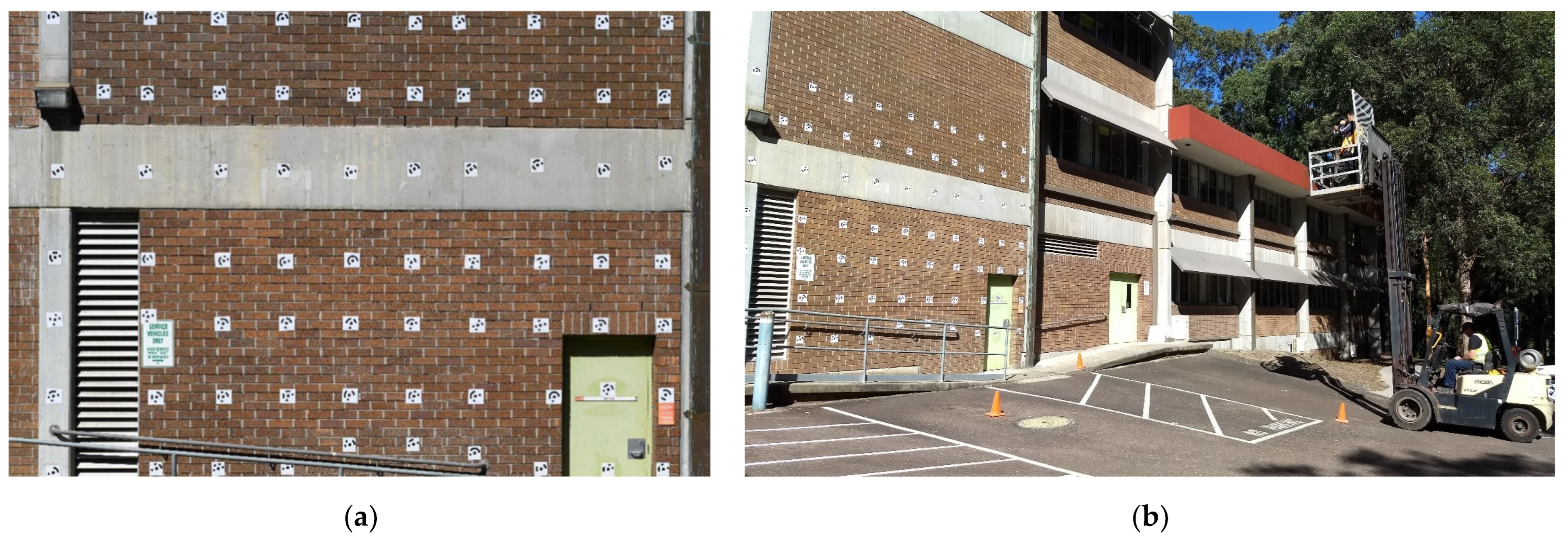
The anticipated camera-to-object distances ranges from 50–100 m. At these distances, it is impractical to establish a calibration field that can be accurately framed for visibility whilst having targets in all areas of the camera sensor. Hence, for this experiment, an ad hoc target field of appropriate size was set up, assuming that for distances greater than a few dozen meters, the focus (and consequently the optical characteristics) of the camera does not change substantially. The camera is housed in a protective box; hence, the optical path of the light rays is influenced not only by the camera’s optics but also by the protective glass panel placed in front of the camera. For this reason, calibration must take place with the camera mounted in a fixed position inside the protective box, which creates further complications by requiring the use of a remote shutter button for image acquisition. The FF calibration of each camera of the fixed monitoring system was performed at the University of Newcastle (NSW, Australia). A north-facing brick wall was equipped (Figure 2) with 70 coded targets placed on approximately seven different heights (the approximate distance between adjacent targets was 65 cm horizontally and 75 cm vertically), encompassing a total area of about 6 × 4.5 m2.
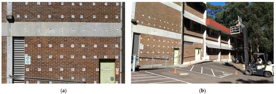
Figure 2.
Full-field (FF) calibration setup: (a) Front view of the coded targets; (b) image acquisition of the target field using a forklift with a safety cage.
The targets were surveyed from two different positions using a Leica TS11 Total Station in a local reference system (expected ground coordinate accuracy of 3 mm). Images were acquired from 15 different positions (Figure 3), at an average distance from the object of approximately 10 m, by varying the acquisition height from the ground using three different forklift extensions within a range of 4 m and rotating the camera in two landscape and two portrait orientations. Consequently, 60 images were acquired in total for each single FF calibration.
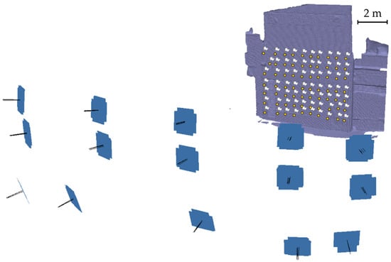
Figure 3.
Image block geometry used for the FF calibration.
All the analytical calibrations were performed using Agisoft Metashape v. 1.8.2 [26]. The proposed calibration procedure represents the most reliable and accurate calibration methodology that can be employed. It should also provide the best results in terms of 3D reconstruction by the monitoring system, provided that the optical parameters of the cameras remain unchanged after the FF calibration. However, it should be noted that this is also the most complex and costly methodology to implement, requiring a calibration field and a series of specialized equipment and facilities to support the operations. If calibration needs to be repeated at regular intervals (which is strongly advisable for long-term monitoring processes), this requires dismantling and transporting the monitoring system to the calibration facility and then reinstalling it on-site.
2.2.2. Multi-Image on-the-Job Calibration—MI
As previously mentioned, the main issue about performing an on-the-job calibration directly on-site using images acquired by the monitoring system originates from the possible unreliable estimation of the parameters due to the intrinsic geometric weakness of the photogrammetric block. This is particularly problematic when the image block consists of just a few camera stations (e.g., just two). Additionally, it is worth noting that each camera has its own calibration parameters, which increases the degree of freedom of the estimation system and consequently its numerical weakness. Moreover, in many cases, the captured object (e.g., a rock wall) is predominantly flat and does not offer depth variations, which is useful for decoupling calibration parameters.
To address this issue, a calibration strategy proposed here involves capturing a series of images during the system installation phase aiming at developing a geometrically more robust photogrammetric block. This occurs before fixing the cameras and their protective box in the intended monitoring position. In many instances, due to safety reasons, it may not be possible to acquire the images at different heights (e.g., using a forklift as in Section 2.2.1), but it is still possible to create a horizontal strip with convergent shots (i.e., photographs from different angles), even by orienting the camera in landscape or portrait mode and using different distances from the object. The placement of coded targets on the object can be equally challenging, but it is still feasible to identify some natural features on the object as GCPs [27]. This is also required during installation to determine the correct georeferencing of the monitoring system. In the experiments, only three GCPs were used for this purpose. From a practical point of view, this strategy requires little effort if compared with the much more complex FF calibration, while also providing good results.
Similar considerations arise about the periodic calibration of the cameras, should the monitoring timeframe be extended. In such a case, the protective camera box needs to be removed from its position and then reinstalled, and correctly reoriented, after completing the calibration process, requiring further efforts. Additionally, the manual positioning of the camera box could result in a slightly different, and undesirable, framing than the previous monitoring period.
The MI on-the-job calibration was conducted by considering different numbers of images (between 15 and 42 images for each camera—see Section 2.3 and Figure 4). In all the procedures, the camera was rotated in different landscape/portrait orientations and was pointing toward the centre of the object with a convergent pose geometry. In all cases, approximately the same camera-to-object distance as the one between the monitoring positions and the object itself was used. All the calibrations were performed using Agisoft Metashape v. 1.8.2 [26]. Despite the possible correlation of some of the parameters, the consistency in the captured object and the block geometry (specifically, the distance from the object) during both the calibration and monitoring stages should significantly reduce the potential deformation of the reconstructed 3D model.
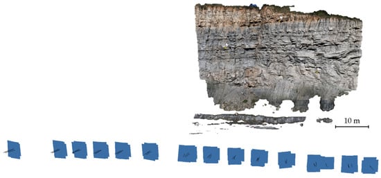
Figure 4.
An example of block geometry used for the MI on-the-job calibration applied to rock slope monitoring.
2.2.3. Point Cloud-Based on-the-Job Calibration—PC
To improve the quality of calibration and ensure good parameter decoupling, using a larger number of GCPs in the BBA could be considered, instead of increasing the number of images composing the calibration photogrammetric block and expanding their spatial distribution (as in the previous section).
However, determining GCPs in the form of well-recognizable natural features on the object using traditional topographic techniques could require considerable effort. To overcome this issue, a new implementation of an aerial triangulation 3D model-controlled procedure is here proposed. In 1988, [28] as well as [29] were the first to discuss the use of DEMs as additional or exclusive control data in image block orientation. More recently, other approaches, indirectly orienting images by comparing the image-derived 3D model with a reference one, have been proposed in [30,31] in 2008 and in [32] in 2018.
The procedure proposed here determines points potentially assimilable to GCPs dynamically (i.e., at each iteration of the bundle block adjustment) by identifying them on a reference 3D mesh or point cloud with a KD-tree nearest point search. In more detail, the orientation routine, at the end of each BBA iteration, extracts the current estimate of all the 3D points (i.e., the tie points) and searches the nearest point on the reference point cloud or the projection on the nearest triangle in the reference mesh. For each coordinate of every tie point, a pseudo-observation is added to the estimation system to reduce its difference from the corresponding coordinate of the nearest point on the reference surface. This is done only if the distance from the reference element is below a preset threshold, filtering out potential outliers. As the BBA iterations progress, these pseudo-observations are assigned progressively higher weights. The procedure is implemented by leveraging the capabilities of the Ceres Solver library [33].
The strategy, in this case, aims at calibrating the cameras using just the two images acquired by the monitoring system and a reference surface model or point cloud, that can be obtained, for instance, using a TLS (Figure 5).

Figure 5.
Example of the image block geometry used for the PC-based and SC on-the-job calibrations applied to rock slope monitoring.
If the object geometry does not change over time or just small, localized changes can be expected (e.g., due to rockfalls on a slope), the reference model can be used for calibrating (and orienting) the monitoring system for several periods. This is probably the most appealing feature (from a practical point of view), since within this strategy, the monitoring stations do not need to be dismantled for calibration and can operate continuously without service interruptions. If an object surface survey needs to be repeated over time, it can still be rapidly done with suitable equipment (for example, with a TLS). It is worth noting that the procedure requires the photogrammetric image block and the reference surface to align in the same reference system: this allows the point search algorithm to identify matches and the orientation BBA to converge. In other words, a set of at least three GCPs surveyed on-site or extracted from the reference surface must be provided for the initial calibration procedure. Most likely, the orientation provided by the initial calibration obtained during installation is sufficient as a first approximate solution to make the BBA converge for all subsequent periods. The use of additional proper GCPs (i.e., points surveyed on-site and identified on the images) should not necessarily improve the quality of the calibration, since many (if not all) of the tie points extracted act as GCPs in the BBA. To verify this assumption, three different GCP configurations were tested in the experiments for this strategy: (i) more than 3 GCPs; (ii) 3 GCPs, which is the minimum number of points required to correctly perform absolute orientation and consequently georeference the monitoring system; and (iii) no GCPs at all. The same configurations were tested for the next calibration strategy.
2.2.4. Self Calibration—SC
The last calibration strategy tested in this study, which is also considered the weakest in terms of accuracy, consists of just using the images coming from the monitoring system. It is, once again, an on-the-job calibration with an image block consisting of only a few (i.e., for the experiments presented, two) images: each image with its own calibration parameters. To distinguish the approach from the strategy proposed in Section 2.2.2., it will be referred to in the following as self calibration (SC), emphasizing the fact that the system is calibrated using exclusively the data acquired for monitoring. In this context, it is crucial to have at least a good number of GCPs for accurate calibration. However, without leveraging the data collected for the PC strategy, it is generally unpractical to identify and measure many natural features.
Therefore, for this type of calibration tests, three amounts of GCPs were tested to evaluate their influence on the results: (i) more than 3 GCPs, considered as a scenario likely applicable in a real-world setting without excessive efforts; (ii) 3 GCPs, which is the minimum number of points required to correctly perform absolute orientation and consequently georeference the monitoring system; and (iii) no GCPs at all. The last two scenarios are motivated by the fact that during monitoring a natural feature, when a new calibration is required, it is not guaranteed that the GCPs identified during the installation phase will still be visible and/or recognizable and still occupy the same positions at a later stage of the monitoring. Let us consider, for example, the monitoring of a landslide where, very likely, all points observed on the object tend to move over time. In the case of movements of the object, the possibility of repeating the control survey was also considered in the previous strategy: it is important to note that the on-site operations and the subsequent GCP identification on the images require a greater effort compared to the previous case, which was, instead, highly automated or automatable. All the analytical calibrations were performed using Agisoft Metashape v. 1.8.2 [26].
As previously emphasized, the main issue in calibrating image blocks with such weak geometric characteristics resides in the potential occurrence of strong correlations among parameters affecting the solution. This may lead to systematic effects (e.g., model deformation) during the 3D reconstruction and, hence, a substantial loss of accuracy. The presence of a larger number of parameters, corresponding to a higher degree of freedom of the BBA resolution system, worsens the phenomenon. Potentially, if the optical–geometric characteristics of the cameras were approximately the same (i.e., calibration parameters did not significantly differ), it would be possible to reduce the problem of parameter correlation by estimating a single camera model for all the monitoring cameras. This calibration method, hereinafter referred to as “Single” to indicate the implementation of a single camera model in the calibration process, was tested for both this and the previous (Section 2.2.3) strategies.
2.3. Test Sites
To evaluate the calibration strategies and assess their actual performances, two test sites were considered.
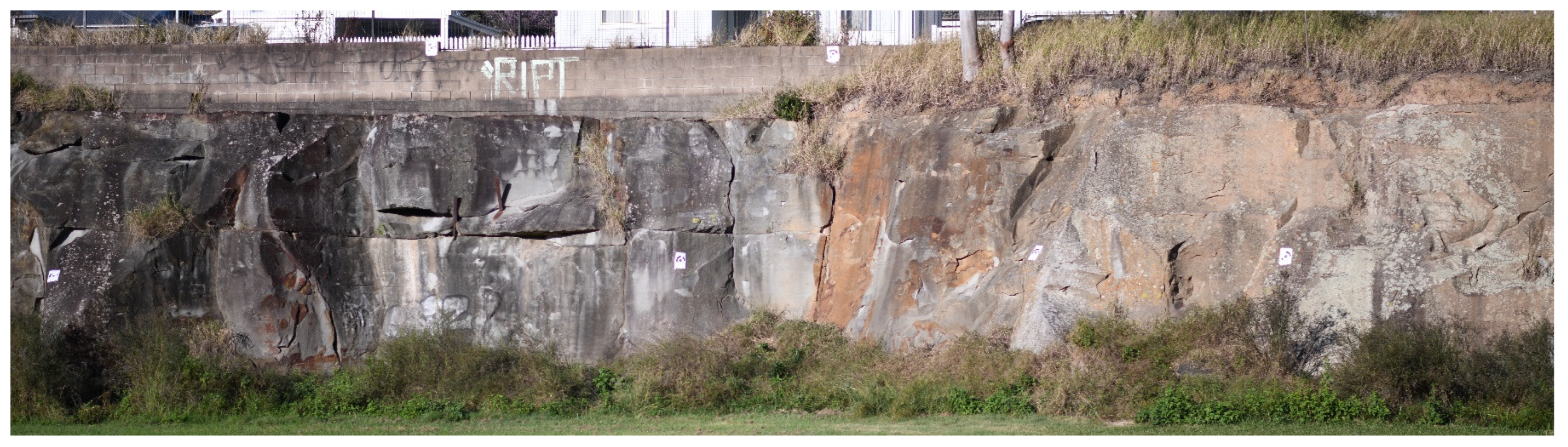
The first (indicated as Site 1) was an abandoned sandstone quarry located at Pilkington Reserve in Newcastle (NSW, Australia). The exposed rock face extended approximately 80 m in length and had an average height of about 6 m (Figure 6). Both a 50 mm and 85 mm lens were considered in the experiments. The area framed by the cameras was approximately 6.5 m high, and 41 and 28 m long for the 50 and 85 mm lenses, respectively.
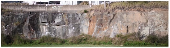
Figure 6.
Overview of the rock face at Pilkington Reserve (Site 1).
The monitoring system was positioned on tripods facing the wall, with the cameras located 73 m away from the wall and spaced at a base length of 18 m in a slightly convergent geometric arrangement.
The level of detail obtainable with each system setup depends on the Ground Sampling Distance (GSD), which can be calculated as follows:
where is the object distance, is the sensor pixel size (for the Nikon D850, this corresponds to 4.36 µm/pixel), and is the expected principal distance of the camera, which can be approximated to the focal length of the optics.
The expected depth accuracy (i.e., the precision along the average optical axis direction of the two cameras) can be estimated by the following equation:
where is the measurement precision of the image coordinates (assumed to be equivalent to ±0.5 pixels) and is the base length (i.e., distance between the two cameras).
The resulting GSDs for Site 1, calculated using Equation (1), were approximately 6.3 and 3.7 mm for the 50 and 85 mm lenses, respectively. The depth accuracy (one sigma), as per Equation (2), was estimated to be around 12.5 mm (equivalent to ca. 2 times the GSD) and 7.4 mm.
Note that, in the following analysis, all the results will be presented both in metric (mm) and GSD proportional units, so that relevant results can be easily transferred to other image blocks with similar geometric configurations (i.e., 0.25 < B/Z < 0.4) but with different distances from the object.
A total of 13 coded targets were attached to the rock face and used as GCPs. The targets were surveyed using the reflectorless mode on a Leica MS60 total station. The Leica MS60 is a hybrid instrument of total station and laser scanner and was also used to produce a point cloud of the rock face with more than 1.1 million points, which corresponds to approximately 4100 per m2 (one point every 1.5 cm on average). The expected accuracy of the surveyed points is approximately 4 mm.
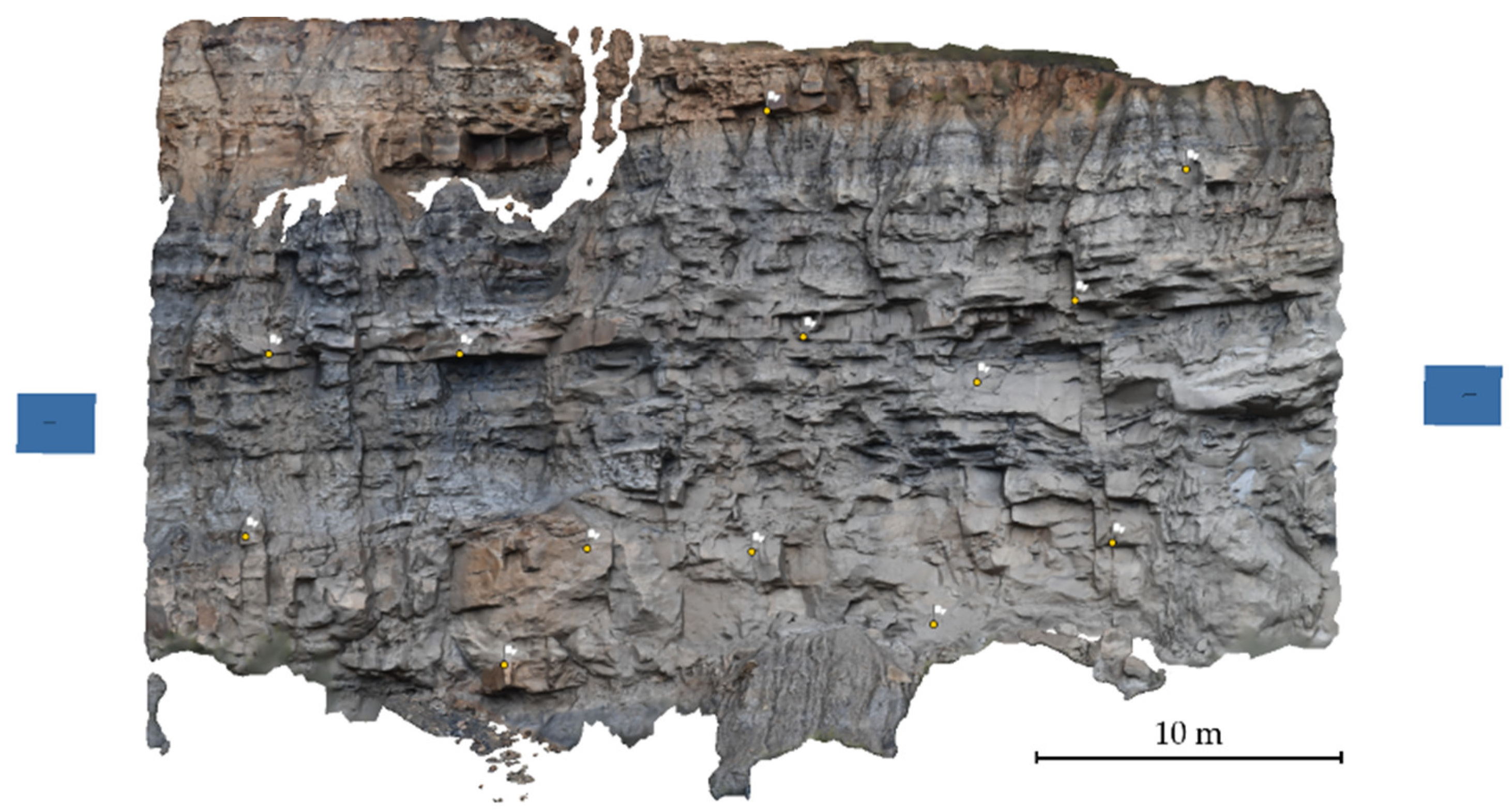
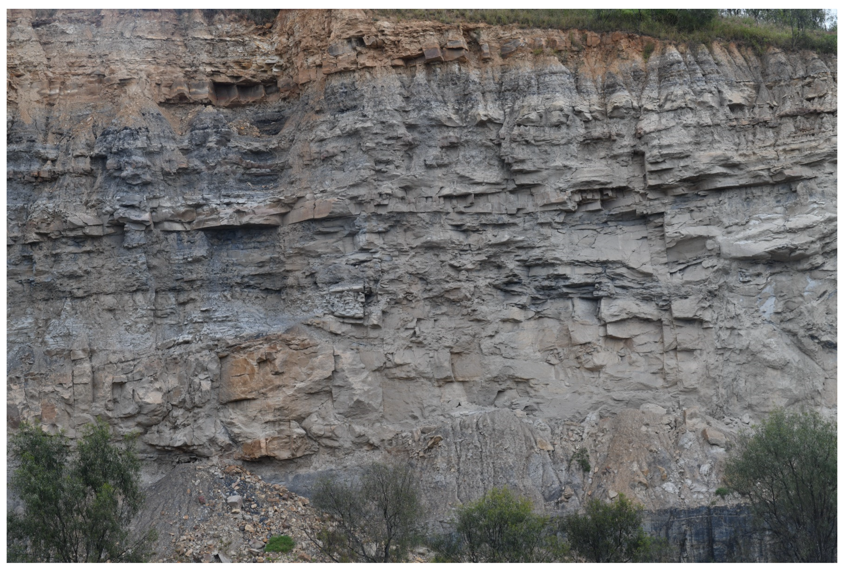
The second test site (in the following indicated as Site 2) was located in a mine site in the Hunter Valley (NSW, Australia). The observed rock face (Figure 7) measured approximately 29 m in height and 35.6 m in width. The calibration data used in the present experiments were acquired on 20 May 2022. In this site, only the 85 mm optics were tested.
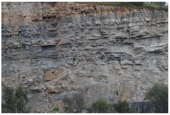
Figure 7.
Overview of the rock face of Site 2.
The two camera units were positioned at a distance of approximately 87 m from the wall. The cameras had a base length of 32.6 m and were set up in a slightly convergent arrangement to maximize overlap. The GSD was 4.5 mm, while the depth accuracy (one sigma) was estimated at 6 mm. A total of 32 GCPs were surveyed on the rock face using a Leica MS60.
To obtain a reference surface to be used as ground truth, a Leica P40 TLS was used, acquiring a point cloud with more than 3.8 million points (ca. 3700 per m2 or 1 point every 1.6 cm). The expected accuracy of the surveyed points, according to the equipment’s technical specifications, is approximately 5 mm.
In both sites, a reflector prism was installed on each camera unit to precisely measure its position with the total station.
2.4. Data Processing
All calibration procedures employed the BBA routines within Agisoft Metashape v. 1.8.2 [26], except for the PC strategy as discussed in Section 2.2.3. PC utilizes an in-house code based on the Ceres library [33]. Nevertheless, it is important to highlight that PC implements the same analytical camera model as Metashape. This ensures perfect interoperability of results and calibration parameters between the two solutions.
The calibration strategies utilized different numbers of GCPs (see Table 1): FF utilized all 70 coded targets on the test field as GCPs, while MI used only three GCPs. For strategies utilizing only the two installed monitoring camera stations (i.e., PC and SC), in addition to the three GCPs used for image block control, as in MI, calibration solutions without GCPs and with a higher number of GCPs (9 for the 50 mm lens, and 7 and 13 for the 85 mm lens at Sites 1 and 2, respectively) were considered to assess whether an increased effort in site surveying could improve calibration results. The calibration utilised a Brown–Conrady [20] frame camera model. It was decided to include parameters corresponding to the first three terms of the radial distortion expansion (K1, K2, and K3) and the two parameters for tangential distortion (P1 and P2) while ignoring affine parameters (B1 and B2) and any additional distortion parameters. Especially for the least redundant strategy (i.e., SC), the increased degree of freedom of the solution would probably lead to stronger parameter correlation and worse results.

Table 1.
Calibration strategies for Site 1 and Site 2.
Upon completion of the calibration procedure, the interior camera parameters obtained were exported and utilized in an identical image block for all tests conducted at the same test site. This image block comprised two images only, with camera centre coordinates accurately measured following the procedure described in [10]. This additional constraint (known coordinates of the camera centre) was utilized as additional ground control. As far as GCP configuration is concerned, the image block had only three control points, positioned at the extreme borders of the object. A final BBA was conducted with all parameters fixed to optimize the orientation solution.
For each block, dense matching was performed using Metashape utilizing the “high-quality” setting, which, in the software terminology, means that images were down-sampled to half their original size during the image matching process. Interpolation was disabled to avoid incorrect surface reconstruction in correspondence with holes, and no decimation was applied to mesh triangles to preserve all the reconstructed faces. In the depth filtering stage, employing the “aggressive” setting, the matching algorithm filtered individual pixels of the depth maps, eliminating those exhibiting different behaviour (i.e., parallaxes) compared to their local neighbourhood. This aggressive approach aimed to filter depth map pixels more frequently to eliminate potentially noisy elements, albeit at the risk of occasionally removing fine details of the reconstruction.
Subsequently, the resulting dense point cloud was exported for comparison with the reference model: for each test site, a ground truth TLS point cloud was acquired (see Section 2.3 for details) and then imported and meshed in CloudCompare [34] using the Poisson Recon Plugin.
The comparison stage encompassed two phases: initially, the photogrammetric point cloud was aligned with the reference TLS mesh through an iterative closest point procedure [35]. This alignment aimed at mitigating or eliminating small systematic translations or rotations that could arise during the orientation stage. Across all tested scenarios, the ICP registration consistently converged within a few iterations (typically 5 to 10 iterations), with final registration residuals closely mirroring the initial ones.
Subsequently, the registered point cloud underwent comparison with the reference DSM using a point-to-mesh algorithm. Specifically, CloudCompare’s cloud-to-mesh (C2M) distance calculation algorithm was employed to ascertain the distance between the two models. Finally, each single point distance to the nearest triangle on the reference ground truth mesh was saved. An automated routine then analysed the distance distribution and computed the average, standard deviation, and Root Mean Square Error (RMSE) of the distances, excluding those points that were too distant from the reference surface. In other words, based on the expected accuracy estimated in Section 2.3, a threshold equal to four times the expected depth precision of ground points was set to filter out possible outliers. The total count of the points in the final reconstruction and the number of the filtered ones were also computed and can be used as an indicator of the completeness of the reconstructed surface.
2.5. Experimental Program
The calibration procedures introduced in Section 2.2 were rigorously tested at Site 1 using both 50 and 85 mm lenses and at Site 2 using the 85 mm lenses. Summarizing Section 2.1, Section 2.3, and Section 2.4, for each of the monitoring configurations (i.e., Site 1–50 mm optics; Site 1–85 mm; and Site 2–85 mm), several calibration strategies were considered:
- full-field calibration (FF)
- multi-image on-the-job calibration (MI)
- point cloud-based on-the-job calibration (PC)
- self calibration (SC).
For the PC and SC strategies, both the influence of using a different number of GCPs supporting the calibration procedure (7/9/13, depending on the site and optics used, 3 GCPs, or 0 GCPs), and the use of a “Single” unique and identical camera model for both the cameras (these calibrations are called PCS and SCS, respectively) was evaluated. For all the other strategies, 3 GCPs and separate camera model parameters for the two cameras were considered. A summary of the calibration strategies for Site 1 and Site 2 is reported in Table 1.
The calibration parameters estimated in each configuration were used in a fixed stereo image block with 3 GCPs and a known camera position as an additional control to obtain a point cloud via dense matching, which was compared with a ground truth TLS-acquired reference mesh. The quality of each configuration was evaluated in terms of spatial and statistical distribution of the differences (i.e., distances) between the photogrammetric point cloud and the ground truth. Since most of the distributions were substantially Gaussian, the average and the RMSE values were considered representative of the distribution itself, along with the number of samples (i.e., points) of the whole point cloud whose distance from the reference surface was not higher than four times the expected depth precision (i.e., the one computed with Equation (2)).
3. Results
3.1. Site 1–50 mm Lens
The results presented in this section detail the comparison between the 3D point cloud generated from stereo-pair images of Site 1 captured with the 50 mm lens using the calibration methods outlined in Section 2 and the 3D reference mesh obtained from the TLS. The comparison was conducted utilising the C2M distance in CloudCompare [34]. Two analyses are presented in the following. The first compared models obtained using three GCPs from the six calibration tests (FF, MI, PC, PCS, SC, and SCS). The second analysis varied the number of GCPs (zero or nine GCPs) for four types of calibration, PC, PCS, SC, and SCS.
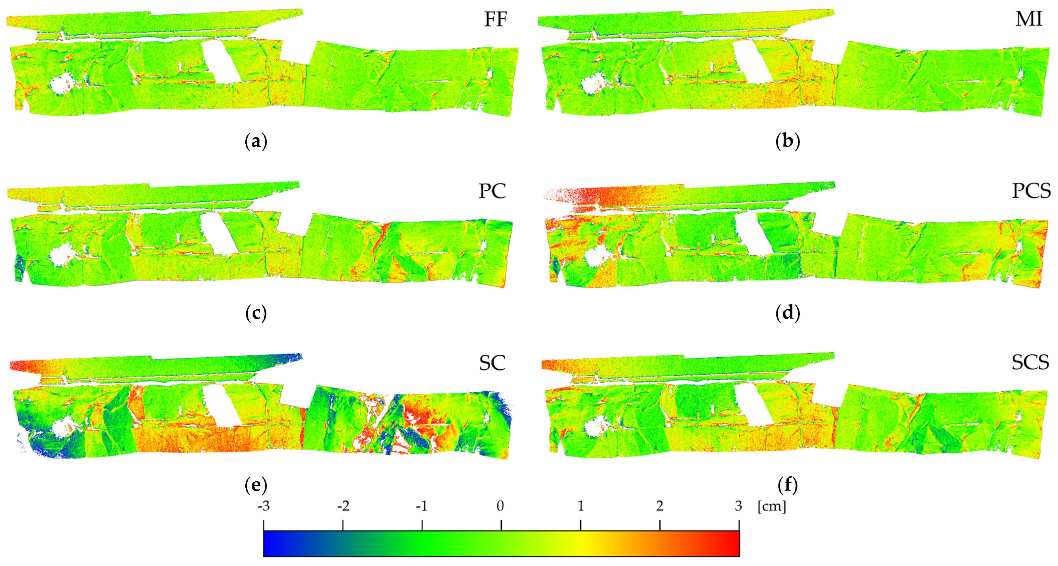
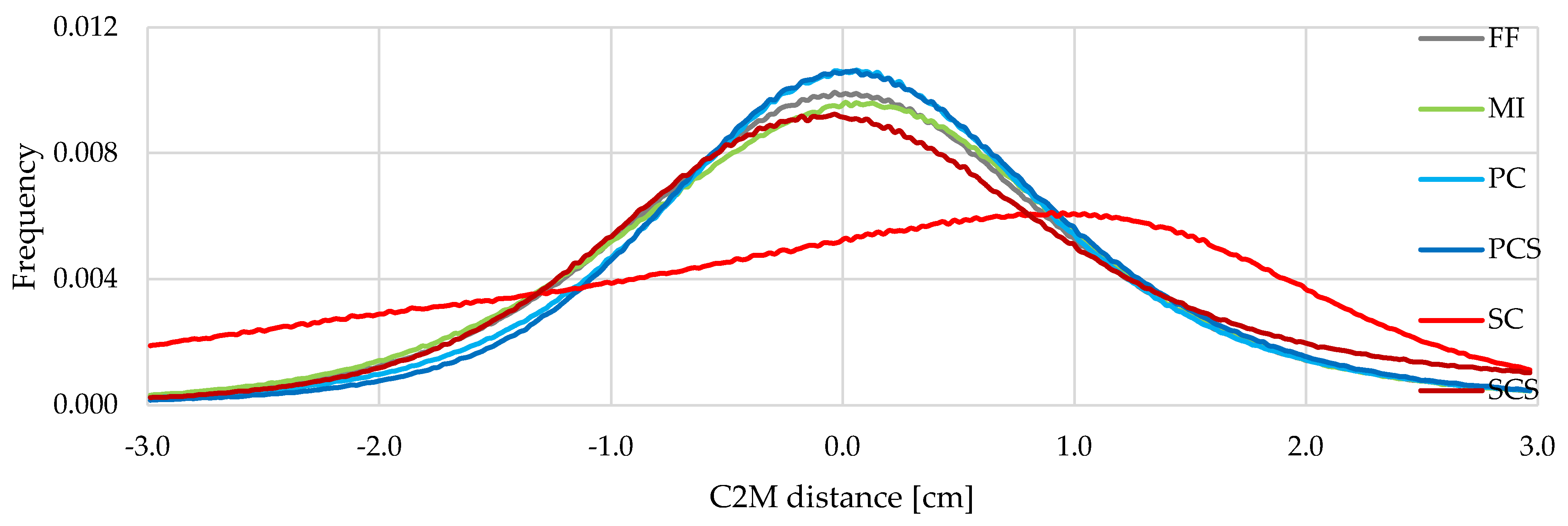
Figure 8 and Figure 9 summarise the results from the C2M of the point clouds processed with three GCPs. Table 2 reports the average distances from the reference mesh, the RMSE, the number of points of the 3D models, and the percentage of points higher than 50 mm or lower than −50 mm. This threshold was determined as four times the expected precision of the monitoring system in ideal conditions. Figure 8 illustrates the frequency distribution of the deviation of the point clouds from the reference mesh, while Figure 9 shows the differences of the point clouds of the object based on a coloured scale from −50 mm to 50 mm. It can be seen that FF, MI, PC, and PCS produce similar results: the RMSE is similar to the GSD (around 12 mm), less than 2% of the points have a difference higher than ±50 mm with a good interpretation of the object (see Figure 9a–d), and the differences have a Gaussian distribution (see Figure 8). On the other hand, the RMSE of SC and SCS is higher (about 24 mm), with a higher number of points (10% for SC and 25% for SCS) bigger than the threshold (±50 mm), presenting local deformations (see Figure 9e,f) and an asymmetric difference distribution (see Figure 8).
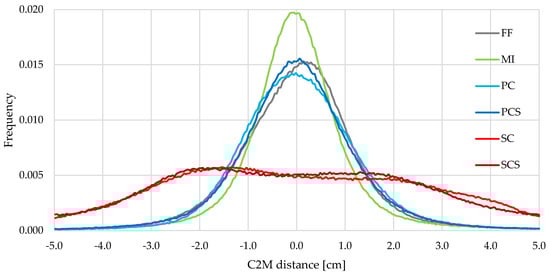
Figure 8.
Distribution of C2M distances for Site 1—50 mm lens using 3 GCPs.
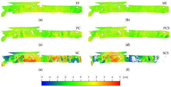
Figure 9.
Results from C2M distance of Site 1—50 mm lens using 3 GCPs. Deviation between the reference mesh and point clouds generated using different types of calibration: (a) FF; (b) MI; (c) PC; (d) PCS; (e) SC; and (f) SCS.
Table 2.
Summary of the results from C2M distance for Site 1–50 mm lens using 3 GCPs.
The analyses using zero or nine GCPs with PC and PCS show similar results compared to the same calibrations using three GCPs. The RMSE is 12.2 (1.9 GSD) and 11.6 mm (1.8 GSD) for PC-0GCPs and PC-9GCPs, while it is 13.2 (2.1 GSD) and 13.4 mm (2.1 GSD) for PCS-0GCPs and PCS-9GCPs, respectively. Hence, as expected, the number of GCPs does not have a big influence on the estimation of the calibration parameters using this type of calibration. Therefore, it can be considered reliable even without GCPs. In contrast, the SC and SCS using zero GCPs do not produce a reliable estimation of the calibration parameters: the RMSE is 28.9 (4.5 GSD) and 26.9 mm (4.2 GSD), respectively. On the other hand, using more GCPs (nine, in this case) improves the performance of the SC and SCS, with an RMSE of 17.2 (2.7 GSD) and 20.7 mm (3.3 GSD), respectively, compared to the 24.2 (3.8 GSD) and 23.8 mm (3.7 GSD) of the same calibrations using three GPSs. Nevertheless, the point clouds from these two calibrations present substantial deformation, in particular for SCS (see Figure 10).

Figure 10.
Results from C2M distance of Site 1—50 mm lens using 9 GCPs. Deviation between the reference mesh and point clouds generated using different types of calibration: (a) SC and (b) SCS.
3.2. Site 1–85 mm Lens
The results presented in this section detail the comparison between the 3D point cloud generated from stereo-pair images of Site 1 captured with the 85 mm lens using the calibration methods outlined in the methodology, and the 3D reference mesh obtained from the laser scanner. As per Site 1–50 mm, two analyses are presented: the first compares models done using three GCPs from the six calibration tests (FF, MI, PC, PCS, SC, and SCS); the second analysis varies the number of GCPs (zero or seven GCPs) for four types of calibration, PC, PCS, SC, and SCS.
Figure 11 and Figure 12 summarise the results from C2M of the point clouds generated using three GCPs only. Table 3 reports the average distances from the reference mesh, the RMSE, the number of points of the 3D models, and the percentage of points higher than 30 mm or lower than −30 mm (threshold determined as four times the expected precision of the monitoring system, in this configuration, in ideal conditions). Figure 11 illustrates the frequency distribution of the deviation of the point clouds from the reference mesh. Figure 12 shows the differences of the point clouds of the object based on a coloured scale from −30 mm to 30 mm. For this test, FF and MI present the best model, with an RMSE of 7.1 and 7.5 mm, respectively. PC, PCS, and, surprisingly, also SCS produce a good model with an RMSE around 8.1 and 9.2 mm. However, PCS presents a localised deformation on the top left of the model (see Figure 12d). FF, MI, PC, and PCS show a Gaussian distribution for the differences while SCS has a lower peak and a slightly asymmetric distribution (see Figure 11). These five calibrations have about 2% of the points higher than the threshold. For this test, SC did not produce a reliable model. The RMSE is 12.9 mm (3.4 GSD), and it has about 9% of the points larger than the threshold (± 30 mm) with several local deformations (see Figure 12e) and an asymmetric difference distribution (see Figure 11).
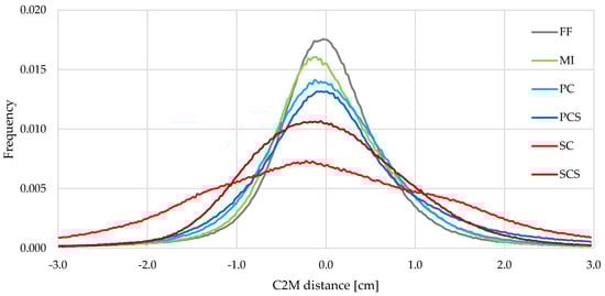
Figure 11.
Distribution of C2M distances for Site 1—85 mm lens using 3 GCPs.

Figure 12.
Results from C2M distance of Site 1—85 mm lens using 3 GCPs. Deviation between the reference mesh and point clouds generated using different types of calibration: (a) FF; (b) MI; (c) PC; (d) PCS; (e) SC; and (f) SCS.
Table 3.
Summary of the results from C2M distance for Site 1–85 mm lens using 3 GCPs.
The analyses using zero or seven GCPs with PC and PCS show similar results compared to the same calibration using three GCPs. PC performs slightly better than PCS. The RMSE is 7.7 (2.1 GSD) and 7.3 mm (2.0 GSD) for PC-0GCPs and PC-9GCPs, while it is 9.3 (2.5 GSD) and 9.3 mm (2.5 GSD) for PCS-0GCPs and PCS-9GCPs, respectively. Once again, the number of GCPs does not have a significant influence on the estimation of the calibration parameters using this type of calibration. Differently from the first test (Site 1–50 mm) presented in Section 3.1, due to a bigger focal lens, the SC and SCS using zero GCPs produce results similar to the ones obtained using three GCPs, with an RMSE of 12.5 (3.3 GSD) and 9.8 mm (2.6 GSD), respectively. On the other hand, using more GCPs (seven, in this case) improves the performance of the SC and SCS with an RMSE of 11.4 and 7.4 mm, compared to the 12.9 and 9.1 mm of the same calibrations using three GPSs. Yet, the point cloud from SC-7GCPs presents substantial deformation on the edges of the model (see Figure 13).
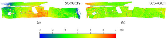
Figure 13.
Results from C2M distance of Site 1—85 mm lens using 7 GCPs. Deviation between the reference mesh and point clouds generated using different types of calibration: (a) SC and (b) SCS.
3.3. Site 2–85 mm Lens
In this section, the comparison between the 3D point cloud generated from stereo-pair images of Site 2 captured with the 85 mm lens using the calibration methods outlined in the methodology, and the 3D reference mesh obtained from the laser scanner are presented. The same two analyses, as per Site 1, were conducted: the first using three GCPs for FF, MI, PC, PCS, SC, and SCS and the second varying the number of GCPs, zero or thirteen GCPs, for the types of calibration PC, PCS, SC, and SCS.
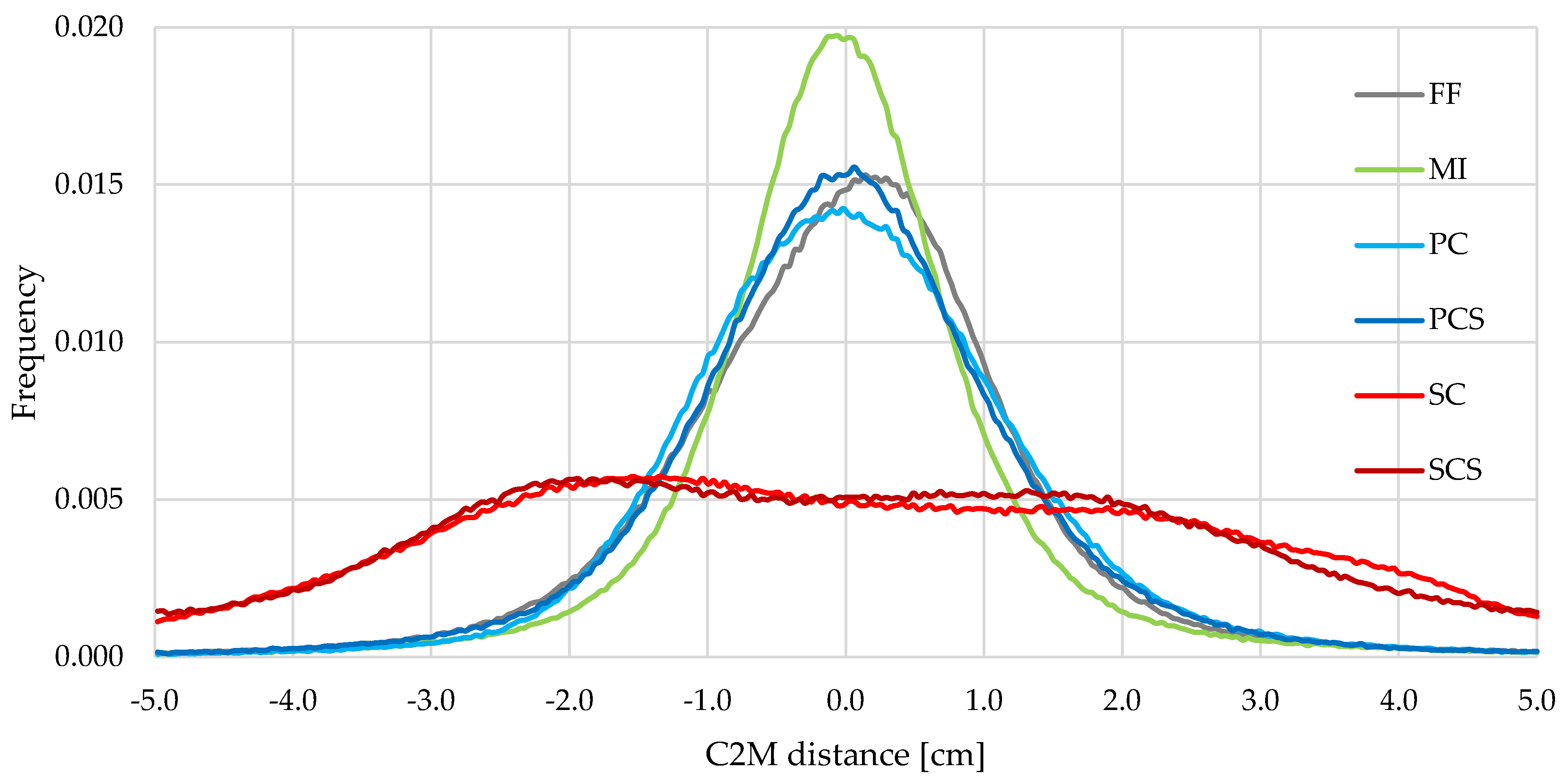
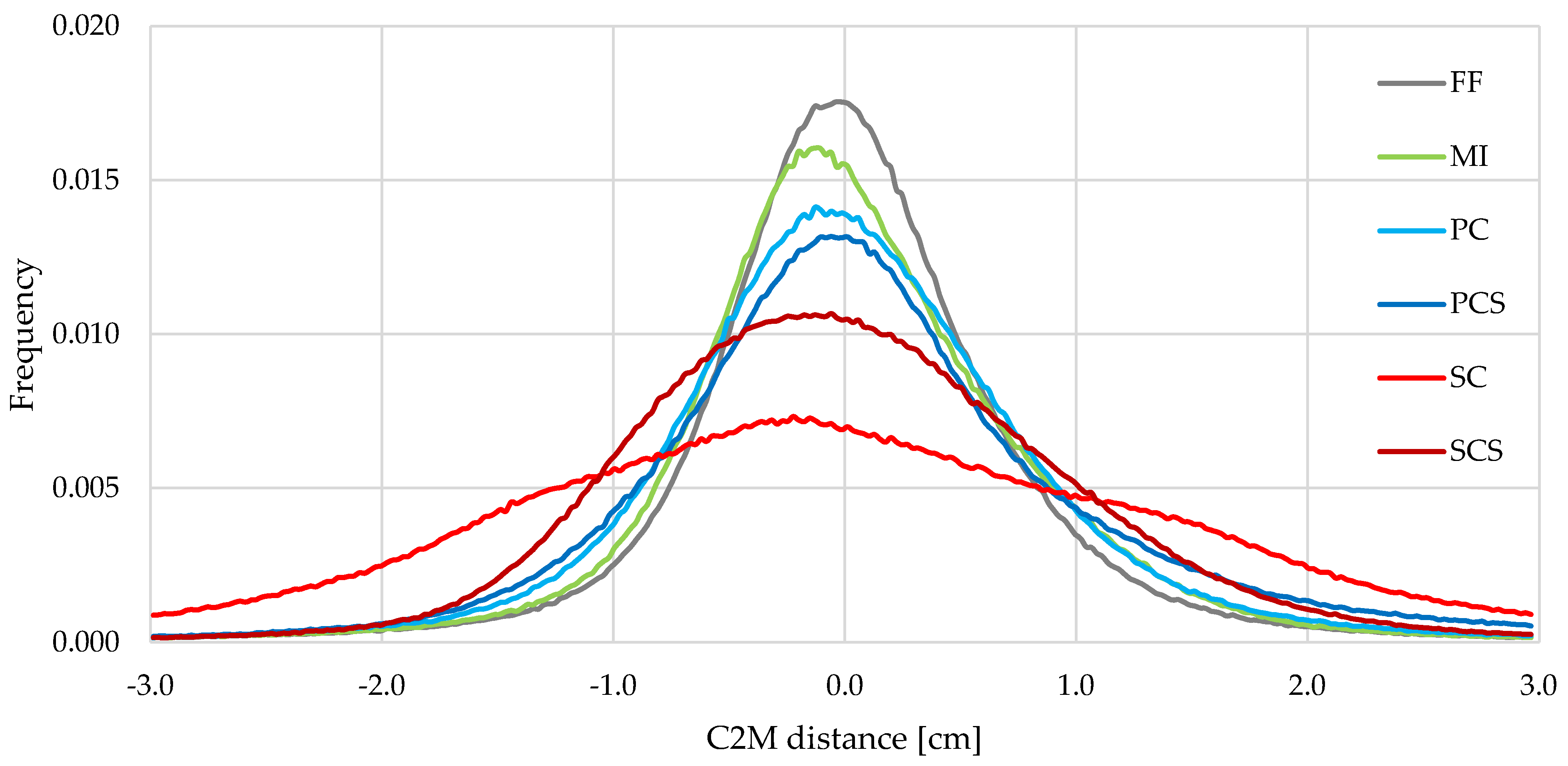
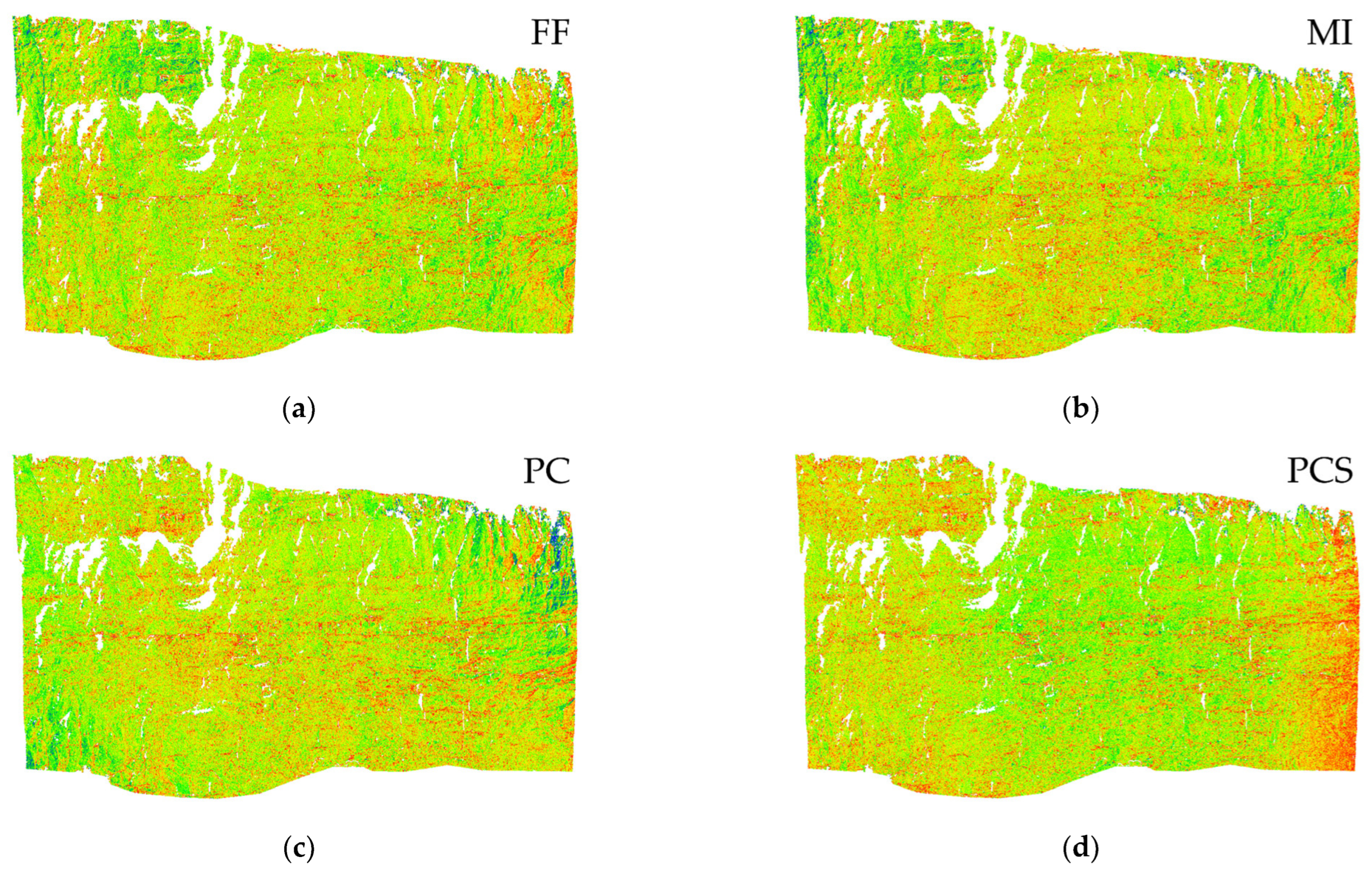
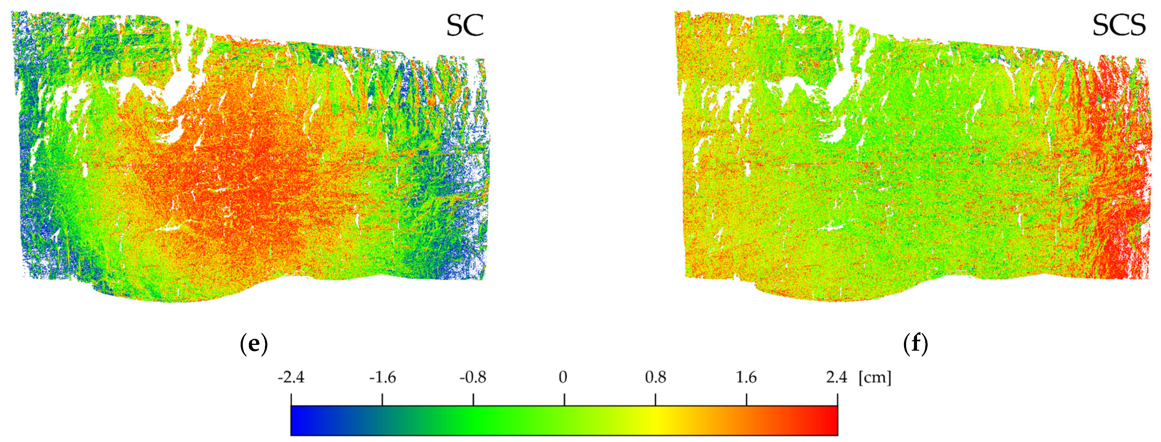
The results from C2M of the point clouds generated using three GCPs are summarised in Figure 14 and Figure 15. The average distances from the reference mesh, the RMSE, the number of points of the 3D models, and the percentage of points higher than 24 mm or lower than −24 mm (threshold determined as four times the expected precision of the monitoring system, in this configuration, in ideal conditions) are reported in Table 4. The frequency distribution of the deviations of the point clouds from the reference mesh is illustrated in Figure 14. The differences of the point clouds of the object based on a coloured scale from −24 mm to 24 mm are shown in Figure 15. For this test, FF, MI, PC, and PCS produce similar results: the RMSE is about 8 mm (1.8 GSD), less than 3.1% of the points have a difference higher than ±24 mm with a good interpretation of the object (see Figure 15a–d) and the differences have a Gaussian distribution (see Figure 14). However, the right-hand side of the SCS model indicates an increase in positive differences (see Figure 14 and Figure 15f). The RMSE is 8.9 mm (2.0 GSD) with a higher number of points (6.5%) bigger than the threshold. For this third test, SC did not produce a reliable model. The RMSE is 11.7 mm (2.6 GSD), and it has about 14% of the points bigger than the threshold (±24 mm) with systematic deformation (see Figure 15e) and an asymmetric difference distribution (see Figure 14).
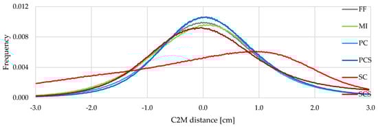
Figure 14.
Distribution of C2M distances for Site 2—85 mm lens using 3 GCPs.
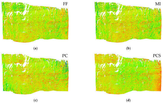

Figure 15.
Result from C2M distance of Site 2—85 mm lens using 3 GCPs. Deviation between the reference mesh and point clouds generated using different types of calibration: (a) FF; (b) MI; (c) PC; (d) PCS; (e) SC; and (f) SCS.
Table 4.
Summary of the results from C2M distance for Site 2–85 mm lens using 3 GCPs.
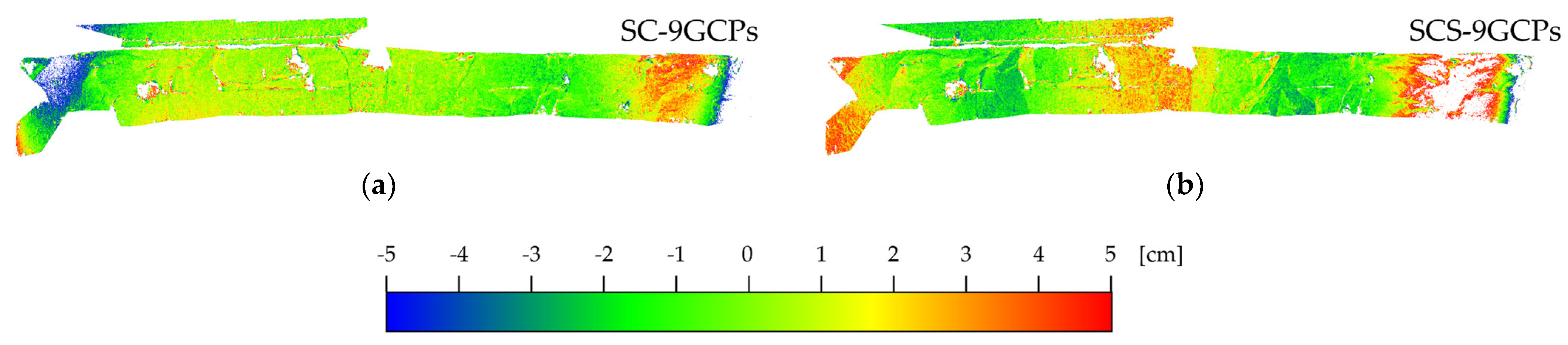
Additionally, for this test, the analyses varying the number of GCPs (zero or thirteen GCPs, in this case) with PC and PCS show similar results compared to the same calibrations using three GCPs. The RMSE is 7.9 (1.8 GSD) and 8.8 mm (2.0 GSD) for PC-0GCPs and PC-13GCPs, while it is 7.8 (1.8 GSD) and 7.7 mm (1.7 GSD) for PCS-0GCPs and PCS-13GCPs, respectively. This test confirms that the number of GCPs does not have a relevant influence on the estimation of the calibration parameters using the PC calibration. As per the first two tests conducted at Site 1, the SC and SCS using zero GCPs do not produce a reliable estimation of the calibration parameters, with an RMSE of 12.8 (2.9 GSD) and 12.6 mm (2.8 GSD), respectively. Using more GCPs (thirteen, in this case) marginally improves the performance of both, SC and SCS, with an RMSE of 10.8 (2.4 GSD) and 8.5 mm (1.9 GSD), compared to the 11.7 (2.6 GSD) and 8.9 mm (2.0 GSD) of the same calibrations using three GPSs. However, the point clouds from SC-13GCPs have a systematic deformation (see Figure 16).
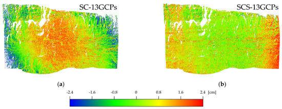
Figure 16.
Results from C2M distance of Site 2—85 mm lens using 13 GCPs. Deviation between the reference mesh and point clouds generated using different types of calibration: (a) SC and (b) SCS.
4. Discussion
4.1. Calibration Parameter Precision and Correlation
In Section 3, the accuracy was obtained by comparing the models generated by the different calibration strategies with a 3D reference model. Determining the accuracy of a fixed monitoring system is critical since it is important to minimize measurement noise and systematic effects, as they can lead to incorrect identification of changes in the monitored object’s morphology. In addition, it is also important to evaluate the levels of uncertainty and the correlation levels among the estimated calibration parameters that each strategy provides. The stochastic model of bundle adjustment, including the type and distribution of observations, determines the precision with which calibration parameters can be estimated. High estimation precision not only ensures a more accurate determination of the actual parameters of the camera model, but also makes the results obtained from the monitoring system more robust and reliable in the face of possible variations in the geometry of the photogrammetric block (e.g., relative translations or rotations between the object and the cameras). On the other hand, high levels of uncertainty in the estimation of calibration parameters or strong correlations among them do not necessarily imply poor results in three-dimensional reconstruction, but can produce model deformation effects that are difficult to predict if the geometric conditions of the block were to change. In other words, even with a high level of parameter estimation uncertainties and strong parameter correlations, accurate results can be obtained. However, in such circumstances, the actual behaviour of the photogrammetric block, if the conditions that have generated such correlations have changed, can make the actual quality of the result unpredictable. In the following, the uncertainty and correlation levels among the estimated calibration parameters will be discussed. For consistency, only the FF using the 85 mm optics and calibrations conducted using the same focal lens on Site 2 (MI, PC, and SC) will be discussed.
In all the scenarios tested in this study, the FF calibration consistently yields the best results in terms of estimation uncertainty and correlation among camera model parameters. This is due to its ability to utilise a highly redundant acquisition geometry, with shots oriented in both portrait and landscape modes, along with a high number of ground control points. For instance, in the calibrations involving 85 mm optics, the uncertainty in the internal orientation parameters is approximately 0.35 pixels (0.02‰ of the estimated value) for the principal distance and around 0.2 pixels for the principal point coordinates. As far as parameter correlations are concerned, apart from the expected high correlations between radial distortion parameters and between principal point coordinates and tangential distortion parameters (typically observed in any photogrammetric block), no significant correlations are noted.
The MI calibration strategy results in similar parameter estimation precision (i.e., 1.1 pixels for the principal distance and 0.25 pixels for principal point coordinates) but with a slightly stronger correlation between principal distance and K1 (16%) and between principal distance and principal point coordinates (ca. 10%). Even if principal point and distance uncertainties are extremely low, the solutions obtained with this strategy in some circumstances (e.g., in the 85 mm—Site 2 test) show much higher differences with respect to the corresponding parameters estimated with the FF calibration. For instance, the principal distance is ca. 70 pixels lower and principal point coordinates differ by ca. 15 ÷ 20 pixels, making the correlation between these parameters the most plausible cause of these changes.
With SC strategies, the parameter estimation precisions are about ten times (principal distance) or one hundred times (principal point) worse than the ones obtainable with FF calibration. Parameter correlations grow considerably: in the 85 mm—Site 2 test, for instance, strong correlations between principal point coordinates and principal distance (more than 50%), between principal distance and K1 (ca. 85%), and between the X and Y components of the principal point (more than 33%) have been obtained. With the PC-assisted calibration, since the image block geometry is largely the same with just a lot more GCP constraints used in the bundle adjustment, represented by the nearest points on the reference surface, a similar result is achieved. In these cases, correlations between principal point coordinates and principal distance are between 30% and 50% and the ones between the two components of the principal point are in the range of 30% to 50%. However, principal distance and K1 show lower correlations than in SC calibration (between 10% and 30%). It is worth noting that the reference surface points used for constraining the solution, in both analysed sites (and, most likely, as one should expect, in any other monitoring site), have a very limited depth range and thus do not provide useful information for improving correlations and estimation precision of the parameters connected to the principal distance. On the other hand, a small improvement in principal point precision (ca. 1/5 ÷ 1/6 of the corresponding SC uncertainty) and radial distortion parameters correlations is assisted.
4.2. Results Analysis and Comparison
Comparing the results obtained from the different site tests with the various calibration strategies implemented, it is easy to notice that the FF strategy consistently provides the best results. This is evident both in terms of the average distance-to-ground truth values of the reconstructed surface (Table 2, Table 3 and Table 4) and in terms of model deformation (which is essentially absent for FF) and spatial distribution of errors (Figure 9, Figure 12 and Figure 13), as well as in terms of parameter estimation accuracies and correlations (see Section 4.1).
In some cases, for example, at Site 1–50 mm, the MI strategy achieves slightly better results than FF, although the differences between the two are very small. However, what needs to be observed, and will be further discussed in the next paragraph, is that the tests conducted did not analyse the stability and validity of calibrations over time and, consequently, how often it is appropriate to repeat the calibration of the monitoring system. While it is plausible to assume that a variation in calibration parameters (due to environmental changes or continuous vibrations affecting the system) may lead to a similar degradation in the quality of 3D reconstruction for all calibration strategies, the practical implications of having to perform a new calibration operation on the system differ substantially among the four analysed strategies.
Analysing the results obtained with the PC-assisted strategy, these consistently align with the FF and MI strategies in all tests conducted, sometimes (for example, at Site 2—85 mm) even providing slightly better reconstruction accuracies (although by less than 5%). The estimation uncertainty and parameter correlation in this case are significantly worse compared to the FF and MI strategies, but this does not seem to negatively affect the results. It should be considered that, with this strategy, the bundle adjustment is forced to obtain a solution that provides a reconstruction as close as possible to the reference surface (in this case, the ground truth). Therefore, it is not surprising that excellent reconstruction results are obtained with this strategy when tie points, and consequently the GCP constraints used in the bundle adjustment, are well distributed over the entire surface of the object. Although this may simply seem like a trick to achieve the desired results, in reality, in a monitoring application like those presented here, where most of the object’s surface undergoes no changes, or in all cases where a reference model is available and the goal is to align the photogrammetric block to it, ensuring maximum adherence, the PC-assisted strategy performs exactly the required task.
When analysing the results with the SC strategy, they generally appear to be the worst. In certain cases (for example, in Site 1–50 mm), systematic reconstruction errors are evident and clearly visible when analysing the error distribution curve (Figure 8) and their spatial representation in false colours (Figure 9e,f). In these cases, using a greater number of GCPs (Figure 10a,b) helps improve the result. In this sense, the PC-assisted strategy is nothing more than using the SC strategy with a very large number of GCPs distributed over the entire surface of the object. A similar consideration explains why the results in terms of calibration parameter estimation uncertainty and parameter correlation are substantially similar in the two strategies, although the greater number of GCPs improves the data obtained with the PC strategy. What differentiates the two strategies is the fact that in the PC-assisted strategy, with a reference surface available, the identification of GCPs is performed automatically.
In the other two case studies (Site 1 and Site 2 with an 85 mm lens), although numerically the RMSE differences are not significantly higher than in the other strategies, it is still possible to notice that with the SC strategy, there are significant deformations in the reconstructed model (Figure 12 and Figure 15e,f). In such cases, it is noteworthy that using the same camera model (i.e., the same calibration parameters) for both cameras yields better results (SCS) compared to when each camera is associated with a different set of parameters (SC). The PC-assisted strategy, on the other hand, shows the opposite behaviour, with more evident model deformations with the PCS strategy compared to the PC one. A possible explanation for this phenomenon may again be related to the correlations between calibration parameters, which are higher in the case of the SC strategy compared to SCS. Conversely, probably due to the greater number of GCPs used, the PC strategy highlights lower correlations compared to PCS.
4.3. Practical Considerations
When considering the practical aspect of calibration, the insights obtained from the experiments are relatively straightforward. It is worth first distinguishing between two cases: 1—the deployment of the monitoring system has a limited time span (a few weeks), and 2—the correct and accurate functioning of the system has to be guaranteed over longer periods. Experience gained by the authors and consensus in scientific literature, along with good practices in photogrammetry, suggest that in the latter scenario, it is advisable to periodically repeat calibration operations, as the optical–geometric parameters of the cameras cannot be considered constant over time.
The FF strategy, although the most reliable and yielding the best results, requires significant efforts, especially when the object being monitored is distant from the monitoring system and long focal length optics are used (e.g., >50 mm). In such cases, a big test field is required to perform the FF calibration. The results obtained seem to indicate that other strategies can achieve comparable results with considerably less effort. If periodic calibration of the system is required, the use of an FF strategy implies long periods of system unavailability. While we do not discourage the use of FF, we suggest its use when the highest level of reliability is required and/or the monitoring system’s operational conditions limit the application of the other alternative calibration strategies. In specific contexts, it could not be possible to spatially develop the photogrammetric block requested by the MI strategy. This could be caused by obstacles reducing the complete visibility of the object from a few specific positions. In other cases, it may be problematic to have a reference surface to apply the PC strategy.
The MI strategy appears to be the best compromise from many perspectives. It provides good estimates of calibration parameters without requiring specific measures of precaution except for spatially developing a good photogrammetric block before fixing the monitoring system cameras in place. Even in the case of repeated calibration procedures, the strategy is rather quick, thus resulting in limited system downtime. However, the act of removing and subsequently repositioning the camera may lead to a slightly different framing of the monitored object after each calibration procedure.
Undoubtedly, considering both the ease of implementation of the calibration strategy and the potentially achievable quality of results, the PC-based method likely represents the best choice. In this scenario, if a 3D reference surface for the monitored object is readily available, the installation and calibration operations of the monitoring system are straightforward. The cameras can be immediately placed in their final positions, and even if a recalibration is required, the cameras do not need to be moved again. In other words, the system can operate without interruptions. Determining the reference surface can be done using instruments such as a TLS or a robotic total station capable of autonomously scanning the object (for example, the Leica MS60 total station used in Site 1 can measure up to 30,000 points per second). The determination of GCPs for the absolute orientation of the photogrammetric block can be performed, if the object’s characteristics allow it, directly on the reference surface. Finally, if few or no movements or displacements of the captured object are expected, the frequency at which a new calibration of the system can be carried out potentially coincides with the image acquisition frequency of the monitoring system.
Finally, considering the use of on-the-job calibration with only monitoring images (SC strategy), while it represents the simplest solution, it also proves to be the most uncertain and least reliable. The results obtained by considering a single set of calibration parameters for both cameras, in the authors’ opinion, should not be misinterpreted. Although the results obtained in some cases may not appear significantly worse than in the other strategies (for example, the results obtained with the 85 mm optics), the uncertainty of estimation, as well as the values of the calibration parameters obtained, indicate that this strategy is not advisable. The results obtained, in other words, while acceptable in terms of the quality of the final 3D reconstruction of the point cloud in two out of three cases, are most likely the result of a fortunate combination of calibration parameters that, albeit far from the real values, produce an overall correct result. Nevertheless, it is important to emphasize that in a continuous monitoring system, it is strategically more important to ensure the reliability of the results rather than their accuracy.
5. Conclusions
This work focuses on investigating the performances of different camera model calibration procedures to be implemented in fixed stereo-photogrammetric monitoring systems in terms of final 3D reconstruction accuracy. The study presents the development of new reliable and effective calibration methodologies that require minimal effort and resources. The camera utilised was a full-format Nikon D850, with a resolution of 45.4 megapixels, equipped with fixed 50 or 85 mm focal length optics. Four different calibration strategies were considered: (i) full-field calibration (FF); (ii) multi-image on-the-job calibration (MI); (iii) point cloud-based calibration (PC); and (iv) self (on-the-job) calibration (SC). To evaluate the calibration strategies and assess their actual performances, two test sites were considered. Based on the results and discussion shown in Section 3 and Section 4, it can be concluded that:
- The FF calibration always gives an accurate estimation of the camera parameters and, hence, accurate 3D models. It is the best choice when the highest level of reliability is required. However, it is not practical to perform this calibration in the field as a controlled space and appropriate equipment are required for this calibration. In addition, it can be time-consuming if it has to be performed regularly.
- The MI calibration appears to be the best compromise between accuracy and practicality. It provides good estimates of calibration parameters, even with few GCPs, as long as the photograms are well-spaced. It can be performed before fixing the monitoring system cameras in place and it can be easily repeated in the field during the monitoring period.
- The PC-based method stands out as the optimal choice, balancing ease of implementation with quality results, when a reference 3D model from a laser scanner is available. It can be repeated without disassembling the monitoring system.
- On-the-job calibration with monitoring images (SC strategy) is the simplest but least reliable option, prone to uncertainty and potential inaccuracies.
Ultimately, prioritising result reliability over absolute accuracy is paramount in continuous monitoring systems.
Author Contributions
Conceptualization, R.R. and D.E.G.; methodology, R.R., D.E.G. and K.T.; software, R.R.; validation, D.E.G., K.T. and E.T.; formal analysis, R.R., D.E.G. and A.G.; investigation, D.E.G. and E.T.; data curation, D.E.G.; writing—original draft preparation, R.R. and D.E.G.; writing—review and editing, A.G. and K.T.; supervision, A.G., K.T. and R.R.; project administration, A.G.; funding acquisition, A.G., K.T. and R.R. All authors have read and agreed to the published version of the manuscript.
Funding
This research was funded by the Australian Research Council (ARC DP210101122) and the Australian Coal Association Research Program (ACARP C29050).
Data Availability Statement
Data supporting the findings of this study are available from the authors on request.
Acknowledgments
This study was financially supported by the Australian Research Council, grant number DP210101122. The support of the Australian Coal Association Research Program (ACARP) and the University of Newcastle facilities is also gratefully acknowledged.
Conflicts of Interest
The authors declare no conflicts of interest.
References
- Stumpf, A.; Malet, J.P.; Allemand, P.; Pierrot-Deseilligny, M.; Skupinski, G. Ground-Based Multi-View Photogrammetry for the Monitoring of Landslide Deformation and Erosion. Geomorphology 2015, 231, 130–145. [Google Scholar] [CrossRef]
- Peppa, M.V.; Mills, J.P.; Moore, P.; Miller, P.E.; Chambers, J.E. Accuracy assessment of a uav-based landslide monitoring system. Int. Arch. Photogramm. Remote Sens. Spat. Inf. Sci. 2016, XLI-B5, 895–902. [Google Scholar] [CrossRef]
- Diefenbach, A.K.; Bull, K.F.; Wessels, R.L.; McGimsey, R.G. Photogrammetric Monitoring of Lava Dome Growth during the 2009 Eruption of Redoubt Volcano. J. Volcanol. Geotherm. Res. 2013, 259, 308–316. [Google Scholar] [CrossRef]
- Rose, W.; Bedford, J.; Howe, E.; Tringham, S. Trialling an Accessible Non-Contact Photogrammetric Monitoring Technique to Detect 3D Change on Wall Paintings. Stud. Conserv. 2022, 67, 545–555. [Google Scholar] [CrossRef]
- Alhaddad, M.; Dewhirst, M.; Soga, K.; Devriendt, M. A New Photogrammetric System for High-Precision Monitoring of Tunnel Deformations. Proc. Inst. Civ. Eng. Transp. 2019, 172, 81–93. [Google Scholar] [CrossRef]
- Hu, J.; Liu, E.; Yu, J. Application of Structural Deformation Monitoring Based on Close-Range Photogrammetry Technology. Adv. Civ. Eng. 2021, 2021, 6621440. [Google Scholar] [CrossRef]
- Unger, J.; Reich, M.; Heipke, C. UAV-Based Photogrammetry: Monitoring of a Building Zone. Int. Arch. Photogramm. Remote Sens. Spat. Inf. Sci. ISPRS Arch. 2014, 40, 601–606. [Google Scholar] [CrossRef]
- Aragón, E.; Munar, S.; Rodríguez, J.; Yamafune, K. Underwater Photogrammetric Monitoring Techniques for Mid-Depth Shipwrecks. J. Cult. Herit. 2018, 34, 255–260. [Google Scholar] [CrossRef]
- Eltner, A.; Kaiser, A.; Abellan, A.; Schindewolf, M. Time Lapse Structure-from-Motion Photogrammetry for Continuous Geomorphic Monitoring. Earth Surf. Process. Landf. 2017, 42, 2240–2253. [Google Scholar] [CrossRef]
- Giacomini, A.; Thoeni, K.; Santise, M.; Diotri, F.; Booth, S.; Fityus, S.; Roncella, R. Temporal-Spatial Frequency Rockfall Data from Open-Pit Highwalls Using a Low-Cost Monitoring System. Remote Sens. 2020, 12, 2459. [Google Scholar] [CrossRef]
- Filhol, S.; Perret, A.; Girod, L.; Sutter, G.; Schuler, T.V.; Burkhart, J.F. Time-Lapse Photogrammetry of Distributed Snow Depth During Snowmelt. Water Resour. Res. 2019, 55, 7916–7926. [Google Scholar] [CrossRef]
- Mallalieu, J.; Carrivick, J.L.; Quincey, D.J.; Smith, M.W.; James, W.H.M. An Integrated Structure-from-Motion and Time-Lapse Technique for Quantifying Ice-Margin Dynamics. J. Glaciol. 2017, 63, 937–949. [Google Scholar] [CrossRef]
- Blanch, X.; Guinau, M.; Eltner, A.; Abellan, A. Fixed Photogrammetric Systems for Natural Hazard Monitoring with High Spatio-Temporal Resolution. Hazards Earth Syst. Sci. 2023, 23, 3285–3303. [Google Scholar] [CrossRef]
- Roncella, R.; Bruno, N.; Diotri, F.; Thoeni, K.; Giacomini, A. Photogrammetric Digital Surface Model Reconstruction in Extreme Low-Light Environments. Remote Sens. 2021, 13, 1261. [Google Scholar] [CrossRef]
- Cosentino, A.; Marmoni, G.M.; Fiorucci, M.; Mazzanti, P.; Scarascia Mugnozza, G.; Esposito, C. Optical and Thermal Image Processing for Monitoring Rainfall Triggered Shallow Landslides: Insights from Analogue Laboratory Experiments. Remote Sens. 2023, 15, 5577. [Google Scholar] [CrossRef]
- Roncella, R.; Forlani, G.; Fornari, M.; Diotri, F. Landslide Monitoring by Fixed-Base Terrestrial Stereo-Photogrammetry. ISPRS Ann. Photogramm. Remote Sens. Spat. Inf. Sci. 2014, II–5, 297–304. [Google Scholar] [CrossRef]
- James, M.R.; Robson, S. Sequential Digital Elevation Models of Active Lava Flows from Ground-Based Stereo Time-Lapse Imagery. ISPRS J. Photogramm. Remote Sens. 2014, 97, 160–170. [Google Scholar] [CrossRef]
- Kromer, R.; Walton, G.; Gray, B.; Lato, M.; Group, R. Development and Optimization of an Automated Fixed-Location Time Lapse Photogrammetric Rock Slope Monitoring System. Remote Sens. 2019, 11, 1890. [Google Scholar] [CrossRef]
- Habib, A.; Detchev, I.; Kwak, E. Stability Analysis for a Multi-Camera Photogrammetric System. Sensors 2014, 14, 15084–15112. [Google Scholar] [CrossRef]
- Brown, D.C. Close-Range Camera Calibration. Photogramm. Eng. 1971, 37, 866. [Google Scholar]
- Parente, L.; Chandler, J.H.; Dixon, N. Optimising the Quality of an SfM-MVS Slope Monitoring System Using Fixed Cameras. Photogramm. Rec. 2019, 34, 408–427. [Google Scholar] [CrossRef]
- Roncella, R.; Forlani, G. A Fixed Terrestrial Photogrammetric System for Landslide Monitoring. In Modern Technologies for Landslide Monitoring and Prediction; Springer: Berlin/Heidelberg, Germany, 2015; pp. 43–67. [Google Scholar] [CrossRef]
- Guccione, D.; Giacomini, A.; Thoeni, K.; Bahootoroody, F.; Roncella, R. A Low-Cost Terrestrial Stereo-Pair Photogrammetric Monitoring System for Highly Hazardous Areas. In Proceedings of the SSIM 2023: Third International Slope Stability in Mining Conference; Australian Centre for Geomechanics, Perth, Australia, 14 November 2023; pp. 803–816. [Google Scholar]
- Luhmann, T.; Robson, S.; Kyle, S.; Boehm, J. Close-Range Photogrammetry and 3D Imaging; De Gruyter: Berlin, Germany, 2019. [Google Scholar]
- Triggs, B.; McLauchlan, P.F.; Hartley, R.I.; Fitzgibbon, A.W. Bundle Adjustment—A Modern Synthesis. In Lecture Notes in Computer Science (Including Subseries Lecture Notes in Artificial Intelligence and Lecture Notes in Bioinformatics); Springer: Berlin/Heidelberg, Germany, 2000; Volume 1883, pp. 298–372. [Google Scholar] [CrossRef]
- Agisoft Metashape: Agisoft Metashape. Available online: https://www.agisoft.com/ (accessed on 9 February 2024).
- Thoeni, K.; Guccione, D.E.; Santise, M.; Giacomini, A.; Roncella, R.; Forlani, G. The potential of low-cost rpas for multi-view reconstruction of sub-vertical rock faces. Int. Arch. Photogramm. Remote Sens. Spat. Inf. Sci. 2016, XLI-B5, 909–916. [Google Scholar] [CrossRef]
- Ebner, H.; Strunz, G. Combined Point Determination Using Digital Terrain Models as Control Information. Int. Arch. Photogramm. Remote Sens. 1988, 27, 578–587. [Google Scholar]
- Rosenholm, D.; Torlegard, K. Three-Dimensional Absolute Orientation of Stereo Models Using Digital Elevation Models. Photogramm Eng. Remote Sens. 1988, 54, 1385–1389. [Google Scholar]
- Gonçalves, J.A. Orientation and DEM Extraction from ALOS-PRISM Images Using the SRTM-DEM as Ground Control. ISPRS Arch. XXIst ISPRS Congr. Tech. Comm. I 2008, 37, 1177–1182. [Google Scholar]
- Chen, L.-C.; Teo, T.; Lo, C. Elevation-Controlled Block Adjustment for Weakly Convergent Satellite Images. ISPRS Int. Arch. Photogramm. Remote Sens. Spat. Inf. Sci. 2008, 37, 761–768. [Google Scholar]
- Cao, H.; Tao, P.; Li, H.; Shi, J. Bundle Adjustment of Satellite Images Based on an Equivalent Geometric Sensor Model with Digital Elevation Model. ISPRS J. Photogramm. Remote Sens. 2019, 156, 169–183. [Google Scholar] [CrossRef]
- Agarwal, S.; Mierle, K.; Team, T.C.S. Ceres Solver 2023. Available online: http://ceres-solver.org/ (accessed on 18 June 2024).
- CloudCompare Homepage. Available online: https://www.cloudcompare.org/ (accessed on 14 February 2024).
- Besl, P.J.; McKay, N.D. A Method for Registration of 3-D Shapes. IEEE Trans. Pattern Anal. Mach. Intell. 1992, 14, 239–256. [Google Scholar] [CrossRef]


Disclaimer/Publisher’s Note: The statements, opinions and data contained in all publications are solely those of the individual author(s) and contributor(s) and not of MDPI and/or the editor(s). MDPI and/or the editor(s) disclaim responsibility for any injury to people or property resulting from any ideas, methods, instructions or products referred to in the content. |
© 2024 by the authors. Licensee MDPI, Basel, Switzerland. This article is an open access article distributed under the terms and conditions of the Creative Commons Attribution (CC BY) license (https://creativecommons.org/licenses/by/4.0/).