Abstract
As the demand for spatial positioning continues to grow, positioning methods based on inertial measurement units (IMUs) are emerging as a promising research topic due to their low cost and robustness against environmental interference. These methods are particularly well suited for global navigation satellite system (GNSS)-denied environments and challenging visual scenarios. While existing algorithms for position estimation using IMUs have demonstrated some effectiveness, there is still significant room for improvement in terms of estimation accuracy. Current approaches primarily treat IMU data as simple time series, neglecting the frequency-domain characteristics of IMU signals. This paper emphasizes the importance of frequency-domain information in IMU signals and proposes a novel neural network, WINNet (Wavelet Inertial Neural Network), which integrates time- and frequency-domain signals using a wavelet transform for spatial positioning with inertial sensors. Additionally, we collected ground-truth data using a LiDAR setup and combined it with the TLIO dataset to form a new IMU spatial positioning dataset. The experimental results demonstrate that our proposed method outperforms the current state-of-the-art inertial neural network algorithms in terms of the ATE, RTE, and drift error metrics overall.
1. Introduction
In recent years, with the rapid growth in the demand for mobile positioning and the prevalence of micro-electromechanical system (MEMS)-based inertial measurement units (IMUs), inertial navigation technology based on IMUs has received widespread attention. Due to advantages such as independence from lighting conditions, low power consumption, and a low cost, inertial odometry algorithms represented by IMU-based approaches have been widely applied to motion estimation for mobile devices, such as unmanned aerial vehicles, augmented reality glasses, virtual reality headsets, autonomous vehicles, and smartphones [1,2].
Current mainstream positioning methods typically include a global navigation satellite system (GNSS), visual odometry, inertial navigation, etc. [2,3,4,5,6]. Among them, the GNSS has the largest positioning range but limited frequency and accuracy and is highly dependent on signals [3,4,7]. Visual odometry methods perform well in terms of accuracy and frequency but rely on lighting conditions and textures and have high computational demands. Inertial navigation methods have virtually no environmental requirements but lower accuracy. In recent years, the rapidly developing visual–inertial odometry (VIO) methods fuse visual and inertial information, exhibiting good accuracy and robustness in most scenarios [8,9,10]. However, VIO still heavily relies on visual information, and when visual tracking fails, the drift and accumulated errors of inertial sensors become exposed [11]. Therefore, it is necessary to study the problem of position estimation based on inertial sensors in challenging scenarios with GNSS signal outages and poor visual conditions.
Some studies have focused on the integration of an inertial navigation system (INS) and a GNSS in a tightly coupled manner using Kalman filter algorithms for sensor-integrated navigation. These approaches have been enhanced by incorporating the Mahalanobis distance criterion, hypothesis testing constraints, and robust factors to improve the Kalman filter. These sensor fusion methods have mitigated the issue of signal loss in a single GNSS sensor and have improved navigation accuracy [12,13,14]. However, such research has concentrated on improving the sensor fusion effects and anomaly handling. In cases where GNSS signals are completely lost, these integrated navigation methods would degrade to the scenario of relying solely on the sensor; hence, in such situations, we still need to investigate the positioning algorithms based on IMUs.
The method of factor graphs is increasingly being used to optimize the positioning accuracy of IMUs [15]. Some studies have utilized factor graphs for the integrated positioning of IMUs with other sensors such as GNSS and LiDAR [16] sensors, while others have improved the IMU preintegration technique by introducing the effects of Earth’s curvature and using factor graph algorithms to fuse different measurement information, thereby enhancing the accuracy of IMU positioning [17]. In addressing the model uncertainties of multi-sensor systems that include IMUs, the Interacting Multiple Model (IMM) approach has demonstrated its unique advantages. The paper [18] integrates adaptive decay and robust unscented Kalman filters within the IMM framework, proposing a new filtering strategy that dynamically selects the optimal sub-filter based on the system mode probability, thereby enhancing the accuracy and robustness of the estimation. The work in [19] further extends the application of the IMM by proposing an adaptive robust filtering method that combines the Mahalanobis distance, which can automatically adjust the filter gain, effectively suppressing the impact of kinematic and observation model errors, and further improving the positioning accuracy of tightly coupled GNSS/INS integrated systems.
Due to the noise and bias present in IMUs, using IMU data for position estimation faces the challenges of accumulated errors and drift [20]. Among inertial sensor position estimation methods, the most common are kinematic-based methods. The IMU records the motion’s acceleration and angular velocity, where acceleration is the second-order derivative of position, and angular velocity is the first-order derivative of orientation. Therefore, by double-integrating the acceleration and single-integrating the angular velocity over a time period, the displacement during that period can be obtained [8]. This method is widely used in traditional inertial navigation systems and VIO. In VIO systems, preintegration methods are usually employed to align visual and inertial sensor data and avoid repeated integration computations [9]. However, most consumer-grade IMUs exhibit noticeable noise errors, and repeated integration operations rapidly amplify these errors, leading to significant accumulated errors and drift.
In periodic motions such as pedestrian dead reckoning (PDR), empirical rules and parameters can be introduced to estimate the stride length [21]. The role of the IMU is to provide acceleration data to directly detect the number of steps taken by the pedestrian. Traditional methods use zero-velocity update (ZUPT), zero-angular-rate update, or step counting to reduce accumulated errors [22,23]. These methods have lower accuracy requirements for the IMU and avoid errors caused by IMU noise. However, their limitation is also evident: the motion must have a specific periodicity or regularity, making it difficult to apply to general motions.
In recent years, with the rapid development of deep learning, data-driven deep learning methods have been applied to inertial position estimation. Unlike traditional methods, deep learning methods do not require integration calculations but directly regress displacements or velocities from accelerations and angular velocities, thereby avoiding rapid error accumulation issues. Consequently, deep learning methods have achieved better accuracy and robustness than traditional methods. IONet [20] was the first to use a long short-term memory (LSTM) network to estimate relative displacements, which were then accumulated to obtain 2D positions. RIDI [24] optimized the bias in IMU data by regressing velocities, then used the optimized data for a double integration to estimate positions. Since angular velocity only required a single integration to estimate motion direction, the error in angle variables was smaller than that in displacements. RoNIN [25] assumed that the rotation data read from the mobile device was accurate, transformed the IMU data into a gravity-corrected coordinate system, and used LSTM, ResNet, and temporal convolutional networks (TCN) to only estimate the velocity. The velocity was then integrated once to obtain displacement, and experiments showed that this method achieved better results. TLIO [26] used a residual network (ResNet) to regress 3D displacements and their corresponding covariances and tightly coupled the neural network with an extended Kalman filter (EKF), enabling the joint estimation of position, orientation, velocity, and IMU bias using only pedestrian IMU data. RNIN-VIO [27] was the first to propose a tightly coupled multi-sensor fusion system that optimized the fusion of visual odometry and inertial neural network position estimation based on ResNet and LSTM, achieving stronger robustness. IDOL [28] proposed a two-stage position estimation method, using a direction module neural network to estimate the motion direction and a position module neural network to estimate the motion displacement, achieving good performance in both direction and position estimation. To address the issue of free head rotation in head-mounted devices, HINNet [29] adopted a dual-layer bidirectional LSTM network and introduced a new “peak ratio” feature as part of the neural network input, enabling the network to distinguish between head rotation and overall motion. HINNet demonstrated that frequency-domain signals could be used to distinguish motion patterns. Wavelet transform methods have been widely applied to signal extraction tasks. For instance, the discrete wavelet transform has been used to extract useful gravitational acceleration signals from signals with a low signal-to-noise ratio [30]. This indicates that wavelet transform methods have a certain noise reduction and signal extraction effect for acceleration signals.
The comparative analysis of various methodologies indicates that neural networks outperform conventional techniques in terms of accuracy and robustness when utilizing inertial data for position estimation. Nonetheless, in environments where visual conditions are optimal, position estimation methods reliant on IMUs are substantially outperformed by those predicated on visual data in precision. Despite the broader environmental adaptability of IMU-based methods, the precision of IMU spatial positioning remains the primary constraint on their advancement. The objective of this paper is to elevate the accuracy of inertial spatial positioning methodologies.
Current inertial odometry research treats IMU data as time-series data, but IMU data can essentially be viewed as one-dimensional signals, which can also be transformed into frequency-domain signals. Through Fourier transform or wavelet transform algorithms, the powerful learning ability of neural networks can be leveraged to extract deeper information from the frequency domain. This paper, based on time-series IMU data, constructs frequency-domain signals through a wavelet transform and uses a neural network to simultaneously learn time-domain and frequency-domain data to predict the motion of inertial sensors.
The key contributions of this article include the development of a novel wavelet-based inertial neural network that outperforms the current state-of-the-art algorithms, TLIO and RNIN, in spatial positioning tasks. This indicates that integrating frequency-domain methods with neural networks can enhance spatial positioning accuracy. We also collected ground-truth data with a LiDAR device and a laser-inertial odometry system, which, together with the TLIO dataset, create a new dataset for inertial spatial positioning.
The rest of this paper is organized as follows: Section 2 describes the overall architecture of our work, the wavelet transform approach, the structure of the neural network, and the setup for algorithm implementation. Section 3 outlines the experimental data and collection process, introduces the baseline algorithms, and defines the evaluation metrics. Section 4 details the experimental outcomes. Section 5 and Section 6 are dedicated to discussing the results and concluding the paper.
2. Architecture
2.1. Overview
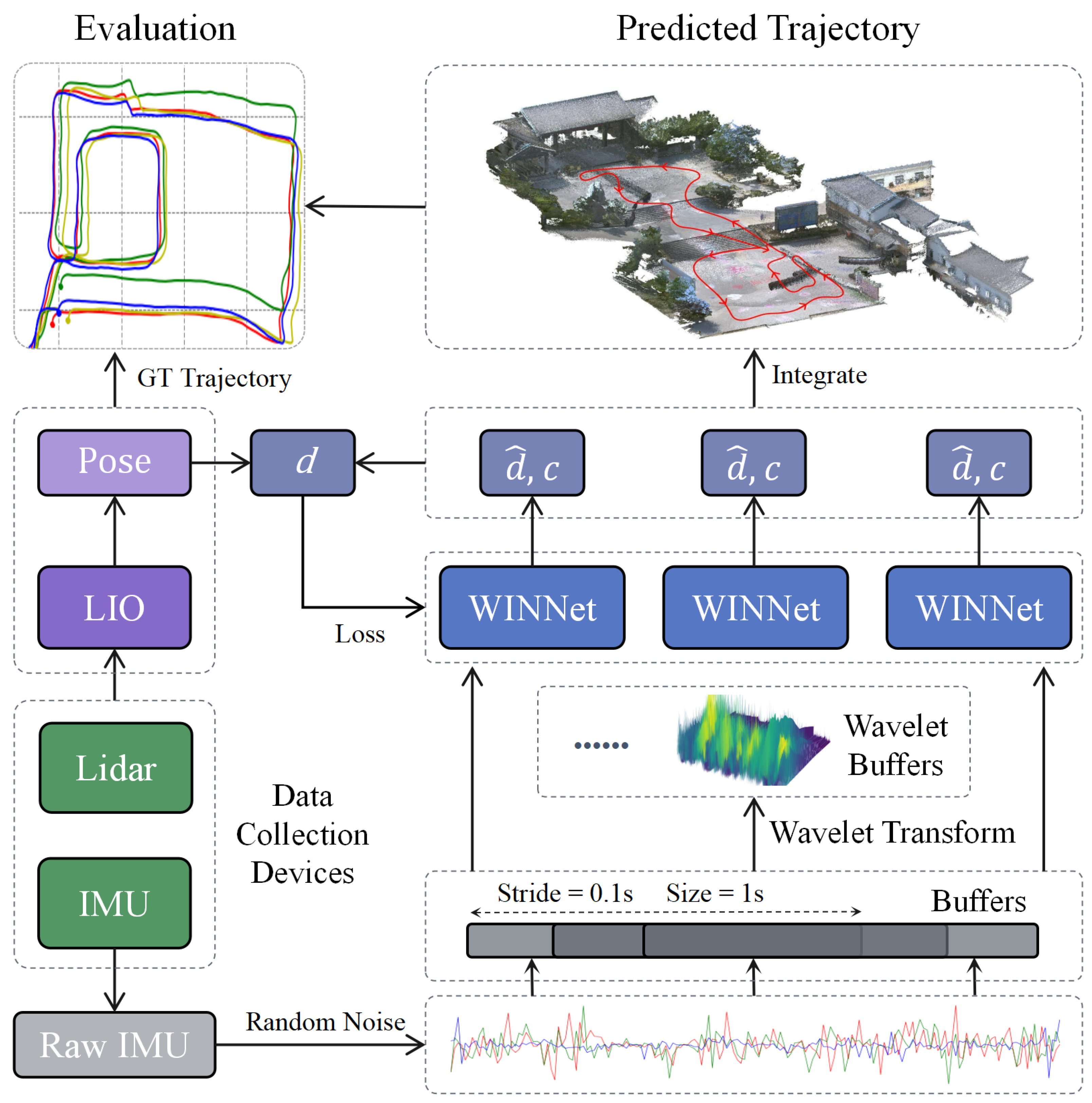
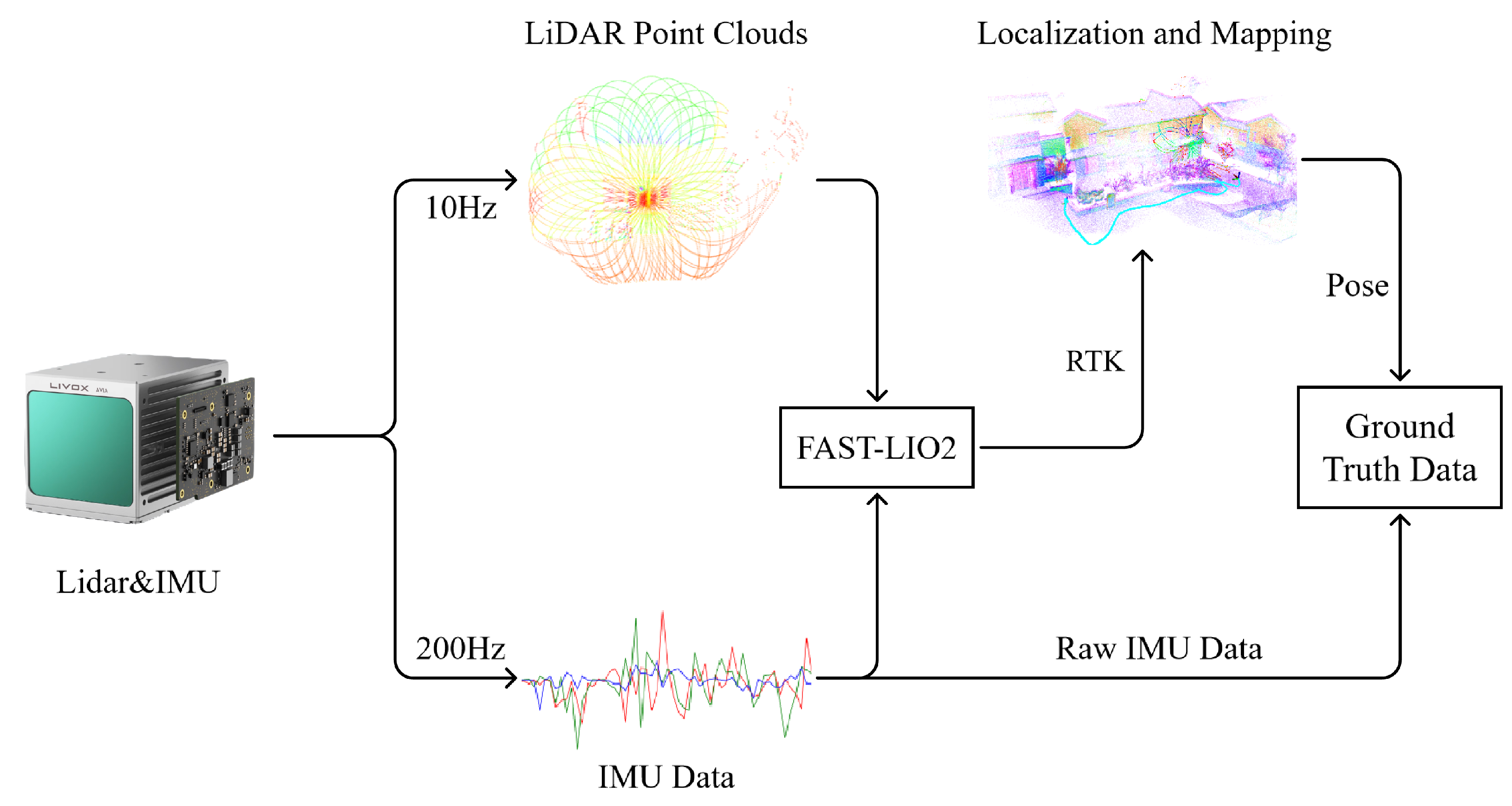
The system architecture is shown in Figure 1. For the IMU data sequence, we used a sliding window of 1 s in length for sampling, with a stride of 0.1 s between windows. After gravity correction and random perturbation data preprocessing, we obtain a 1 s IMU buffer data. These data are simultaneously fed into the wavelet transform module and the WINNet module. The wavelet transform module converts the IMU buffer data into time–frequency data, which are then input into the WINNet module for feature learning. The WINNet module receives both the original IMU buffer data and the time–frequency data output from the wavelet transform module and outputs the displacement and confidence weights for the current buffer window, thereby calculating the trajectory.

Figure 1.
Overview of the methods in this paper, including the creation of a dataset, the development of an inertial spatial positioning algorithm, and the assessment of the positioning trajectory’s accuracy. d represents the true displacement, denotes the displacement estimated by the algorithm, and c signifies the confidence weight output by the neural network WINNet.
2.2. Wavelet Transform
The raw IMU data are time-domain signals with different frequencies coupled together, making it difficult to extract waveform features. In the frequency domain, different waveforms can be well separated, facilitating feature extraction. Therefore, we considered using neural networks to learn the motion patterns inherent in the frequency-domain signals, which aided in the final motion spatial positioning.
The Fourier transform is the most common algorithm for time–frequency-domain conversion, while the basic principle of the wavelet transform is to decompose the original signal using a set of basis functions (i.e., wavelet functions) to obtain a series of wavelet coefficients reflecting the signal’s characteristics at different scales and times. Wavelet transforms are widely used in applications such as action detection. We chose to use the wavelet transform for the IMU signal transformation for the following reasons:
- The Fourier transform requires the assumption that the signal is stationary, whereas IMU data in practical applications are usually non-stationary and contains many signal transients. The wavelet transform does not require the signal stationarity assumption and can handle transient signals well.
- The wavelet transform provides joint time–frequency information, meaning it can reveal the frequency changes occurring at specific times, while the Fourier transform cannot provide this time localization information. It can locate both time and frequency and is highly sensitive to signal transients, which the Fourier transform cannot represent well.
- The wavelet transform can analyze signals at different scales, enabling it to capture both coarse and fine signal features. This is particularly useful for analyzing signals with multi-scale structures or rapidly changing details.
The wavelet transform extracts signal features at different scales and time locations by scaling and translating a mother wavelet function. It can be represented as the inner product operation between the signal and a set of wavelet basis functions. For the discrete wavelet basis functions of an IMU signal, they can be represented as:
where j is the scale parameter, determining the wavelet frequency, k is the translation parameter, determining the wavelet time location, and is the scale factor, ensuring equal energy of the wavelet basis functions across different scales.
The discrete wavelet transform can be viewed as decomposing the signal into a linear combination of a series of scaling functions and wavelet functions; thus, the IMU signal can be expressed as:
where is the scaling function, representing the low-frequency approximation of the signal, is the scaling coefficient, representing the low-frequency approximation coefficient of the signal at scale , and is the wavelet coefficient, representing the high-frequency detail coefficient of the signal at scale j.
The discrete wavelet transform of the IMU signal is as follows:
where represents the discrete wavelet coefficients, which are the projection coefficients of the signal onto the scale j and time location k. denotes the complex conjugate of .
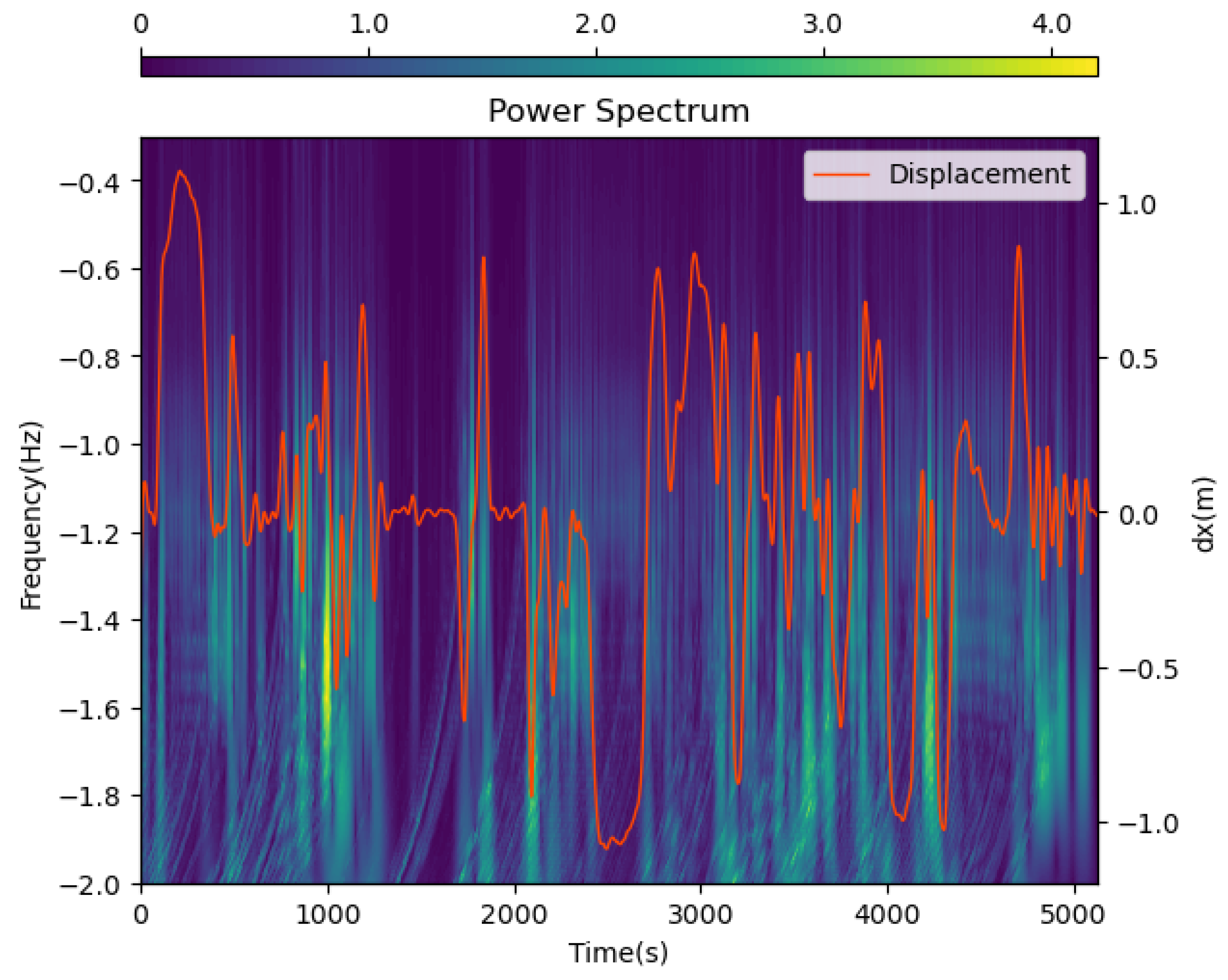
We visualize the data after wavelet transformation in Figure 2. The closer the background color is to purple, the lower the signal intensity, and the closer to yellow, the higher the signal intensity. The orange line represents the ground-truth displacement of the object along the x-axis. We can observe a strong consistency between the ground-truth displacement and the wavelet transform signal patterns: the times of intense signal fluctuations closely match the times of drastic changes in motion displacement. This indicates that frequency-domain information can reflect motion changes and contribute to uncovering inherent motion patterns. Moreover, the wavelet transform not only reveals frequency-domain information but also clearly shows the correspondence between frequency and time, which is something the traditional Fourier transform cannot achieve. The time–frequency signal obtained after wavelet transformation greatly assists the neural network in extracting deep-level motion patterns and trajectories.
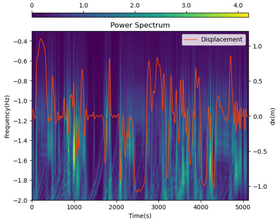
Figure 2.
Visualization of wavelet transform data. The x-axis represents the time axis, the left y-axis represents the frequency axis, the right y-axis represent the displacement, and the color represents the signal intensity. The orange line represents the ground truth displacement of the object along the x-axis. The data of frequency and time have been transformed by a log function to better visualize the data.
2.3. Neural Network
The overall neural network architecture is shown in Figure 3. The architecture of the network is structured to include an input layer, parallel residual modules, a fusion layer, and an output layer. The input layer accepts measurements from the IMU as well as data that have undergone wavelet transformation. The parallel residual modules are composed of four 2D and one 1D residual blocks. The fusion layer initially merges the outputs from the two sub-networks, which are then fed into the fully connected layers. Two fully connected layers are responsible for outputting the displacement’s confidence weights. The parallel residual modules are constituted by a pair of concurrent ResNet sub-networks, each featuring analogous network layers. The work [31] demonstrated that frequency-domain data obtained from the Fourier transform could distinguish different types of motions, indicating the ability of frequency-domain data to extract motion pattern features. Compared to the Fourier transform, the wavelet transform has better adaptability for non-stationary signals and does not lose the time information corresponding to frequencies, which is more conducive for the network to learn motion features. Therefore, we used the wavelet transform to obtain time–frequency data, and a 2D sub-network learned the motion pattern features hidden in the time–frequency data, while a 1D sub-network learned the motion information from the raw IMU data. Both sub-networks had residual layers composed of four residual blocks, and the output of the last residual block was fused in the fusion layer. Then, the fused features were input into two identical fully connected layers to estimate the displacement and confidence weights corresponding to the current buffer window, thereby calculating the trajectory. The confidence weights helped construct the loss function and optimize the network training process. The confidence weight was calculated as:
where is the abstract function of the part of the network that outputs the confidence weight, is the input data, is the output of the fully connected layer, and is the sigmoid function, which maps the output to the range (0,1]
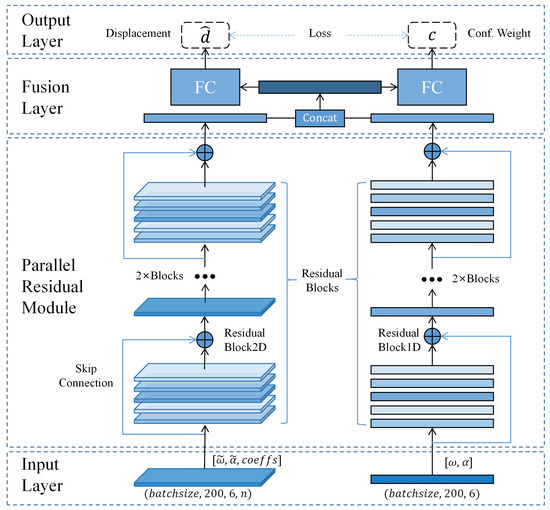
Figure 3.
WINNet architecture. symbolizes angular velocity, symbolizes acceleration, and correspond to the data derived from the wavelet transformation of and , respectively. signifies the calculated displacement, and c represents the confidence weight associated with the network’s output.
The loss function was designed to minimize the error between the predicted trajectory and the ground-truth trajectory. The loss function was defined as:
where N is the number of samples in the buffer window, is the ground-truth displacement, is the predicted displacement, and is the confidence weight of the displacement. is the weight coefficient of the confidence weight, which was used to balance the influence of the confidence weight on the loss function. The loss function was weighted by the confidence weight, ensuring that the network focused more on the regions with a higher confidence weight.
3. Experiments
3.1. Dataset Collection
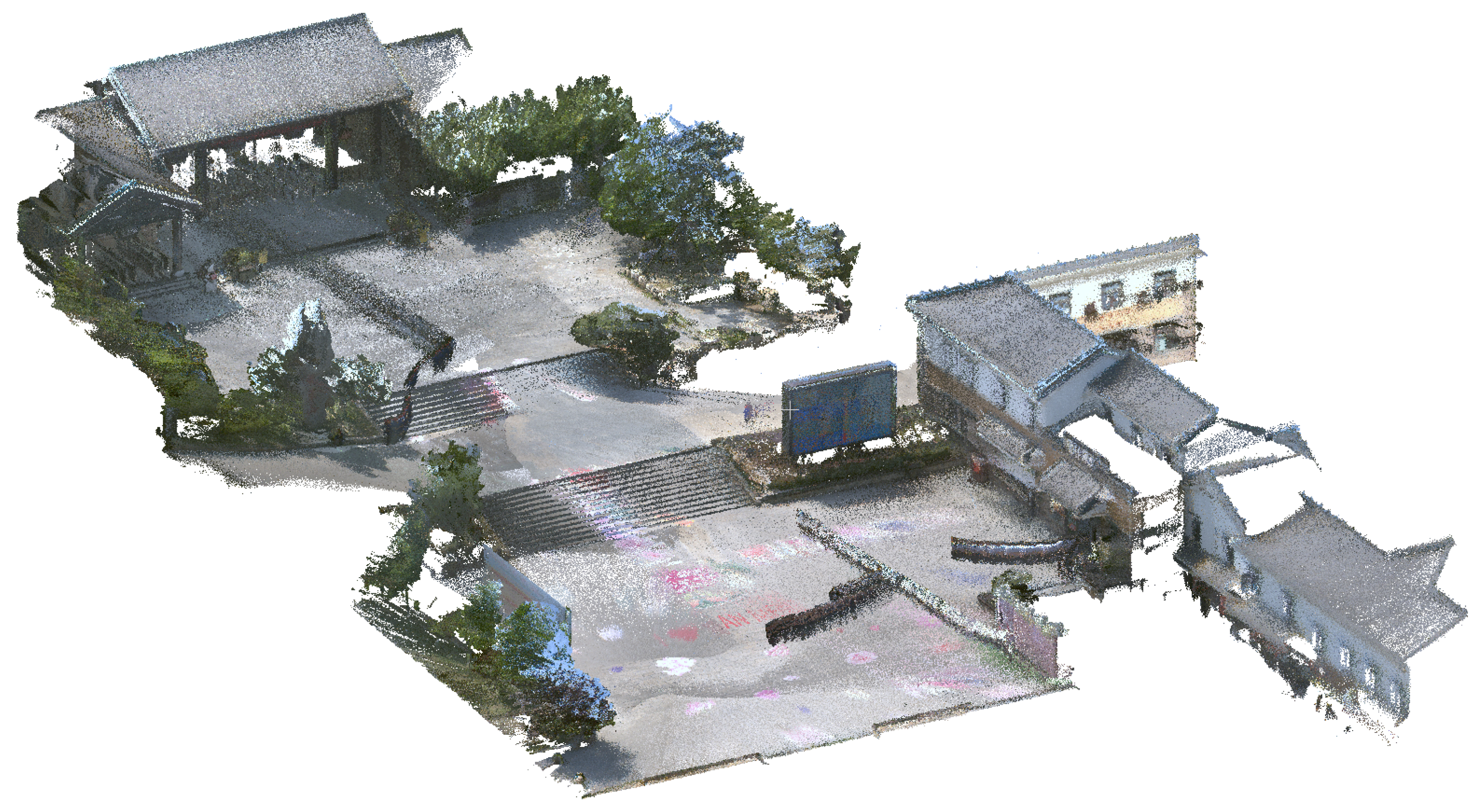
FAST-LIO2 [32] was employed to generate ground-truth data. This method is founded on an efficient tightly coupled iterative Kalman filter that estimates the motion state of the sensor, characterized by its robustness, precision, and high efficiency. It achieves accuracy at the centimeter level, significantly surpassing the positioning precision of purely inertial sensors, making it suitable for acquiring ground-truth data. We conducted an experiment by carrying a novel solid-state LiDAR integrated with an IMU around a construction area spanning approximately 14,000 square meters. The area was open and flat, consisting of a small plaza and several residential buildings. The 3D mapping of the data collection area is shown in Figure 4. The collection device synchronously acquired a LiDAR point cloud and IMU data at frequencies of 10 Hz and 200 Hz, respectively. The IMU model used in this setup was the BMI088. RTK was used to collect ground control points and obtain the global coordinates of the data collection area so that we could evaluate and improve the accuracy of the ground-truth data. The root-mean-square error (RMSE) of the ground-truth data was 0.057 m, which was sufficient for the subsequent evaluation of the algorithm. The device used in our experiments is listed in Table 1. The data collection process is illustrated in Figure 5.
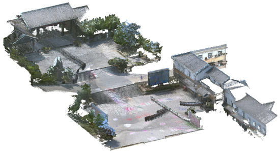
Figure 4.
The 3D mapping of the data collection area.

Table 1.
Devices used in our experiments.
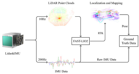
Figure 5.
Data collection process. The device was held by the user, and the LiDAR and IMU data were collected simultaneously. The ground-truth dataset consisted of raw IMU data and position data obtained from the LiDAR inertial odometry system.
We supplemented our dataset with the TLIO dataset, which was collected using a Bosch BMI055 IMU and a camera, containing various daily activities of pedestrians, depicting a wide range of personal motion patterns and IMU system errors. The ground-truth positions were estimated using a visual–inertial filtering algorithm. Since the TLIO dataset was collected using a head-mounted device, differing from the handheld motion patterns of our LiDAR device, it increased the overall diversity of the dataset.
3.2. Implementation
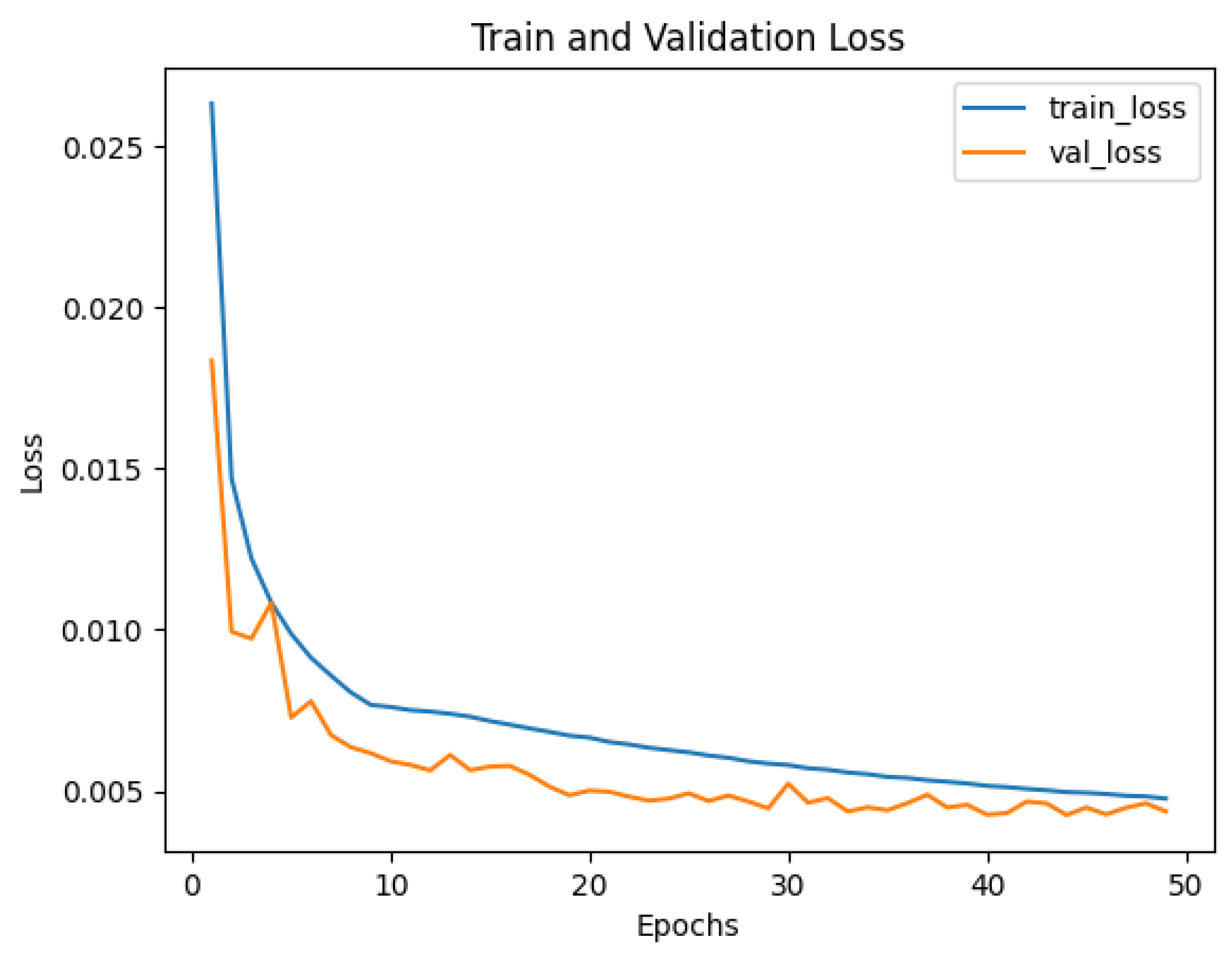
The ground-truth data were derived from laser inertial odometry calibrated by high-precision RTK, which generated three-dimensional positional coordinates at a frequency of 10 Hz for each time point, thereby obtaining the ground-truth trajectory data. We divided approximately 36 h of data samples into training, validation, and test sets in a ratio of 7:2:1. The raw 6-axis IMU data were fed into the testing method, where the algorithm output the displacement for the corresponding time period, and the displacement was then integrated to obtain the predicted trajectory. Since the IMU operated at a frequency of 200 Hz while the ground-truth data were at 10 Hz, we used a 0.1 s window as the fundamental unit to align the data. For the 200 Hz IMU data, a sliding window of length 200 with a stride of 10 was used for sampling the input data. Considering the 6 variables of the IMU data and a batch size of 1024, the input data shape for each window was 1024 × 200 × 6. Since the IMU device rotated during motion, we recalculated the rotation relative to the first frame for each frame, aligning the gravity direction. After gravity alignment, we also added random perturbations during the training process to simulate installation errors and structural vibrations of the IMU device in real scenarios, enhancing the network’s robustness. The Adam optimizer was used for network training, with an initial learning rate of 1 × 10 and a dropout of 0.5 for the fully connected layers. Training was performed on an RTX 3090 GPU, taking approximately 130 min to fully converge around the 35th epoch. The training loss curve is shown in Figure 6.

Figure 6.
Training loss curve. The x-axis represents the number of epochs, and the y-axis represents the loss value. The blue line represents the training loss, and the orange line represents the validation loss.
3.3. Baseline Methods
We compared the proposed WINNet algorithm with the following algorithms:
- TLIO: The TLIO algorithm is the state-of-the-art inertial odometry algorithm. It uses a ResNet network to regress 3D displacements and their corresponding covariances, tightly coupled with an EKF to estimate position, orientation, velocity, and IMU bias using only pedestrian IMU data.
- RNIN: RNIN is a part of the RNIN-VIO algorithm, which is the state-of-the-art visual–inertial odometry algorithm. We removed the visual odometry part and only used the part of the inertial neural network named RNIN. It uses a ResNet and LSTM neural network model to combine relative and absolute loss functions, achieving stronger robustness.
3.4. Evaluation Metrics
The experiment was conducted on the collected dataset, with 10% of the data selected as the test set to evaluate the following metrics:
ATE (Absolute Trajectory Error): Reflects the position error between the estimated and ground-truth values, computed as the root-mean-square error (RMSE). The ATE is calculated as:
RTE (Relative Trajectory Error): Reflects the error between estimated and ground-truth positions within a unit time, unaffected by accumulated errors since only the deviation within a unit time is considered. The RTE is calculated as:
Drift (Final Relative Drift): Reflects the relative drift between the final estimated and ground truth position. The drift is calculated as:
4. Results
In order to ascertain the spatial positioning capabilities of our proposed methodology, a duo of experimental series were executed utilizing the ATE, RTE, and drift metrics as benchmarks. The initial series of experiments served the purpose of juxtaposing our method against contemporary algorithms, specifically TLIO and RNIN. The comparative performance of these algorithms was evaluated across a collection of 20 test trajectories. The corresponding experimental outcomes are articulated in Figure 7, Figure 8, Figure 9, Figure 10, Figure 11, Figure 12, as well as Table 2, Table 3.
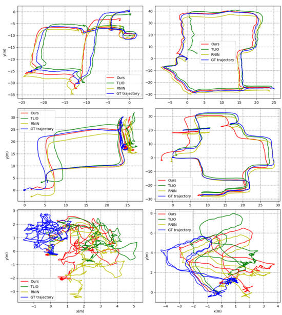
Figure 7.
Some examples of trajectory plots with different difficulty levels. The x-axis represents the horizontal position, the y-axis represents the vertical position, and the color represents different methods. The GT trajectory is the ground-truth trajectory, which was produced by the LiDAR device and LiDAR inertial odometry system. Note: The experimental outcomes yielded positional coordinates across three orthogonal dimensions, encompassing x, y, and z. Nonetheless, the trajectory plots within the figures are confined to the plane of the x and y axes. This exclusion of the z-axis is deliberate, stemming from the negligible magnitude of error observed in that direction, which complicates comparative analysis. Therefore, in the interest of enhancing the legibility and clarity of the presentation, the z-axis has been intentionally excluded from the graphical illustrations.
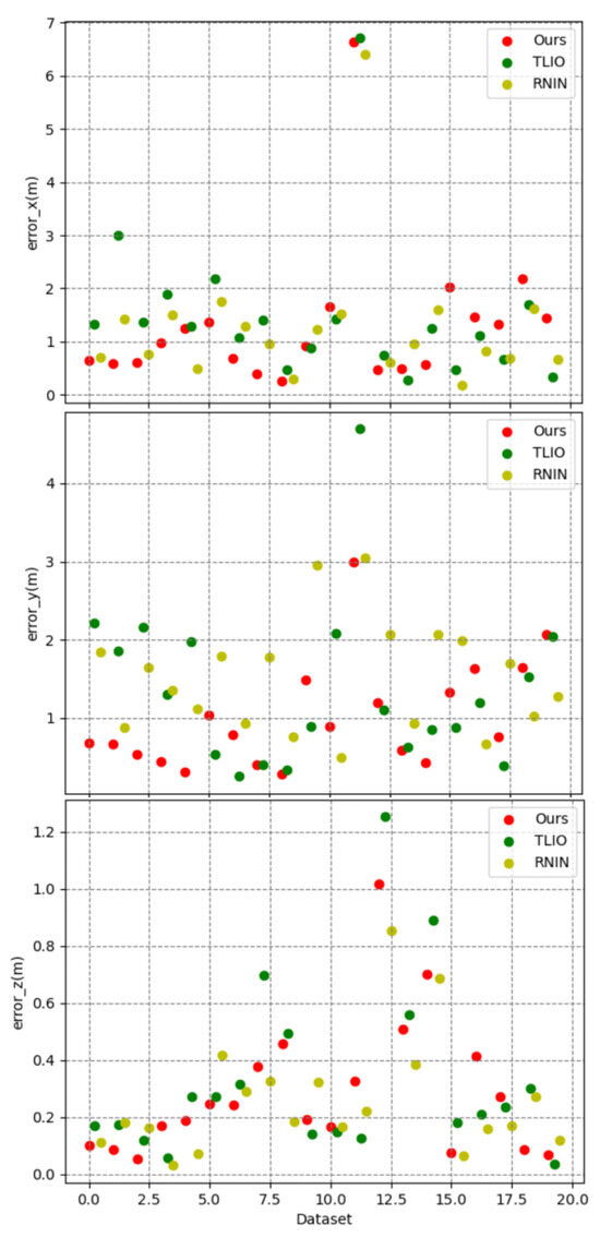
Figure 8.
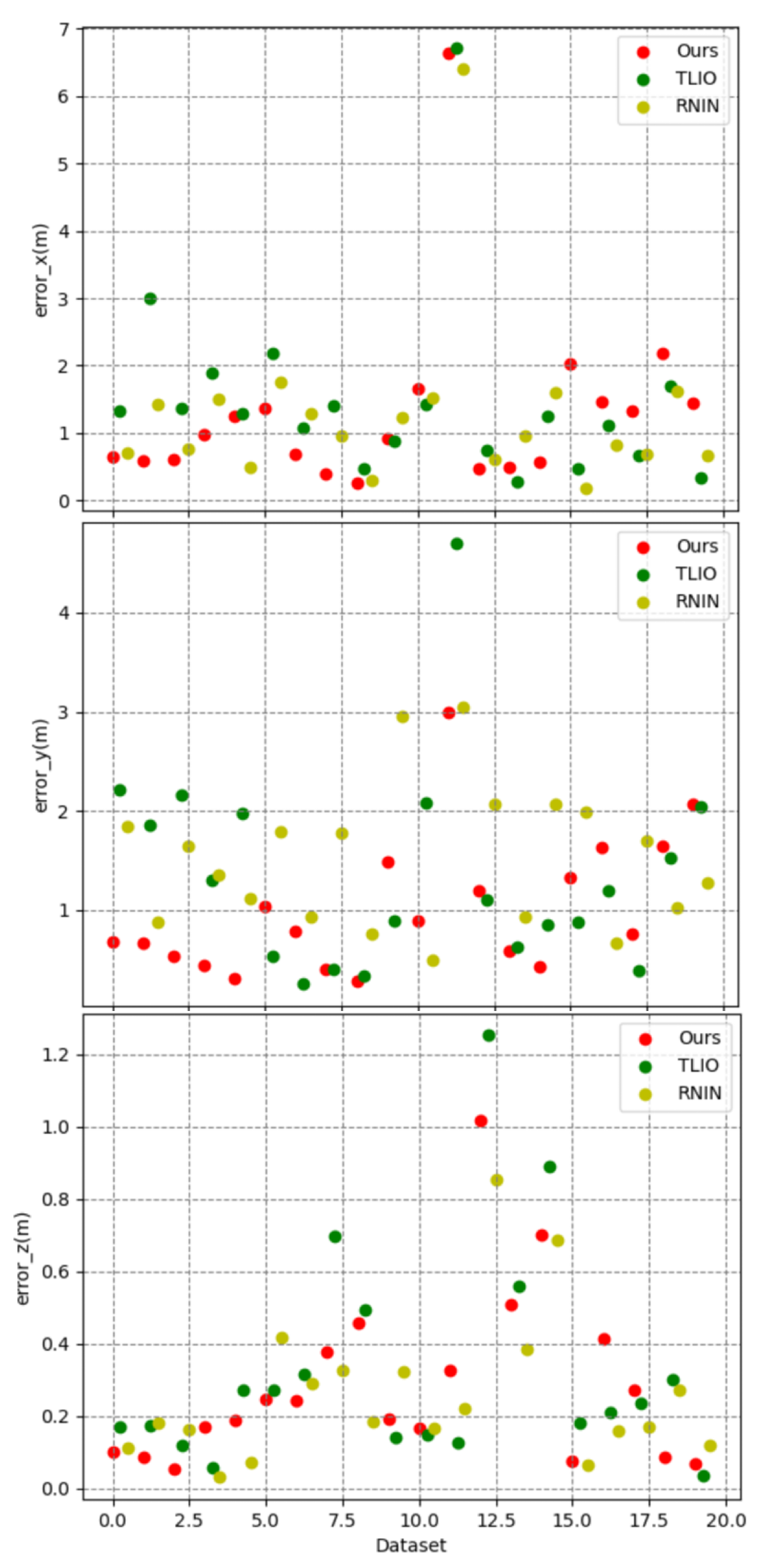
Error in x, y, and z. The x-axis represents the dataset, the y-axis represents the error value, and the color represents the method.
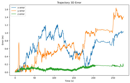
Figure 9.
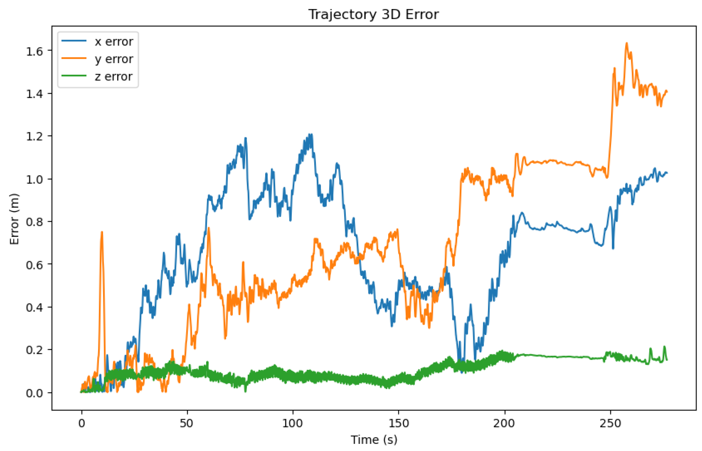
Three-dimensional error of a selected trajectory predicated by our method. The x-axis represents the time, the y-axis represents the error value, and the color represents the three axes.
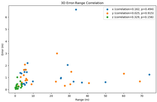
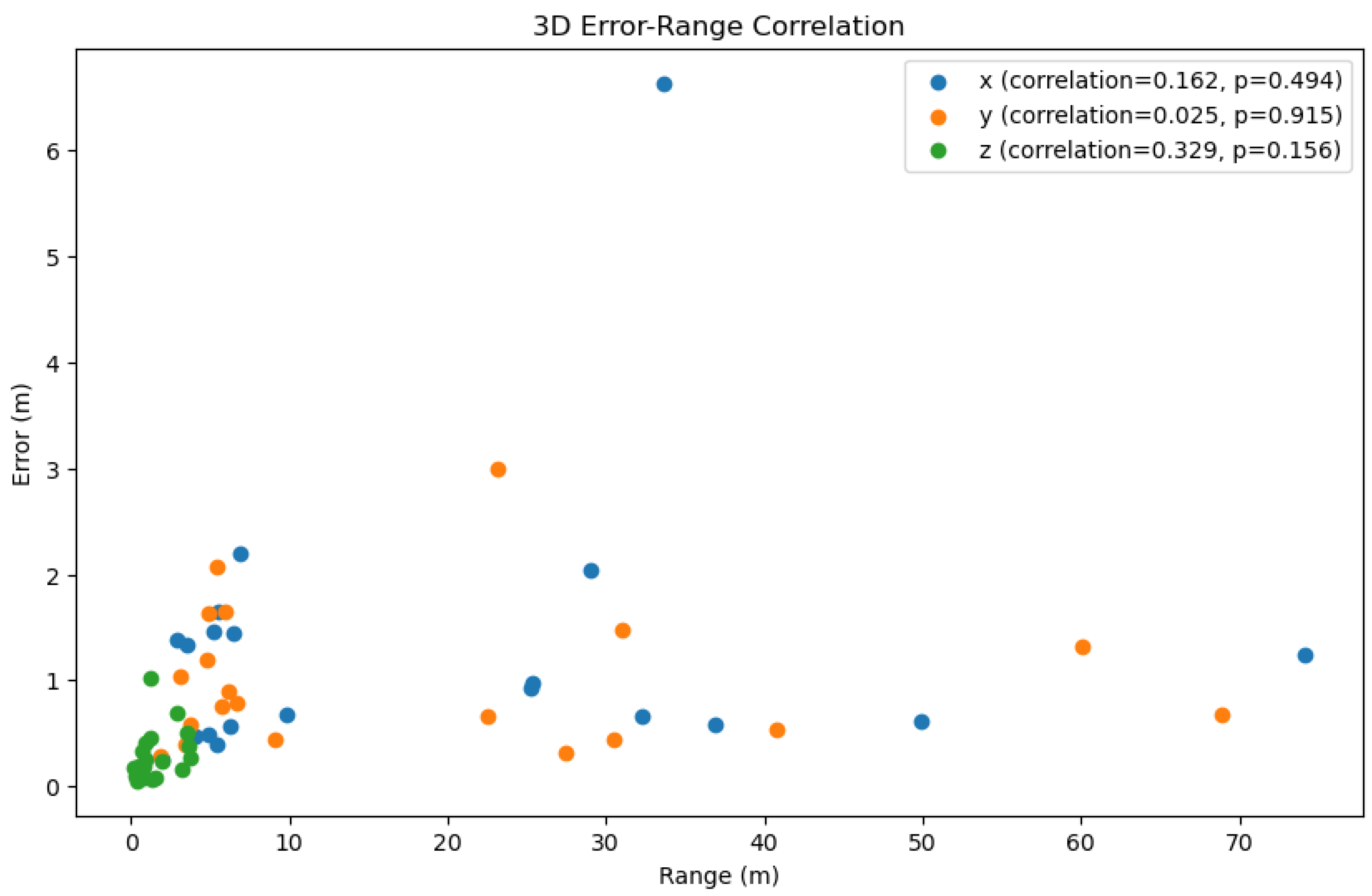
Figure 10.
Correlation between the error and the range of x, y, and z. The x-axis represents the range of the dataset, the y-axis represents the error value, and the color represents the three axes. Note: The correction between the error and the range of x, y, and z was calculated by the Pearson correlation coefficient. The p-value of the correlation indicates that the correlation was statistically significant when p < 0.05. The greater the positive correlation, the more pronounced the cumulative effect of the error.
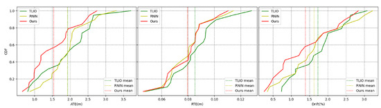
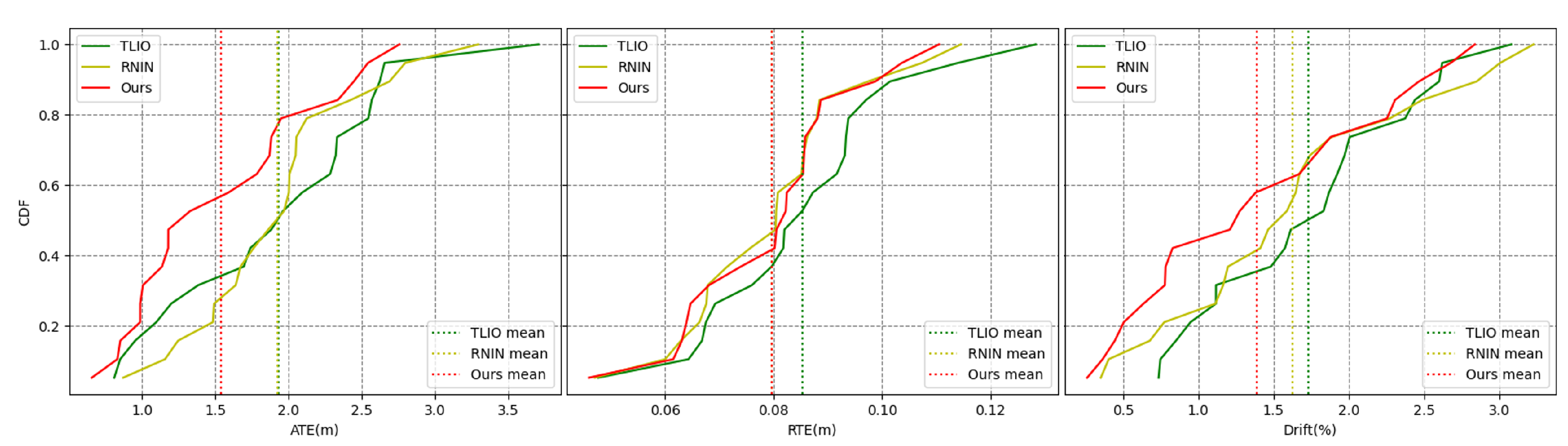
Figure 11.
Error accumulation curves. The x-axis represents the error value, the y-axis represents the cumulative distribution, and the color represents the method.
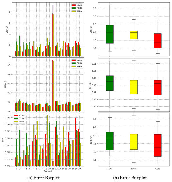
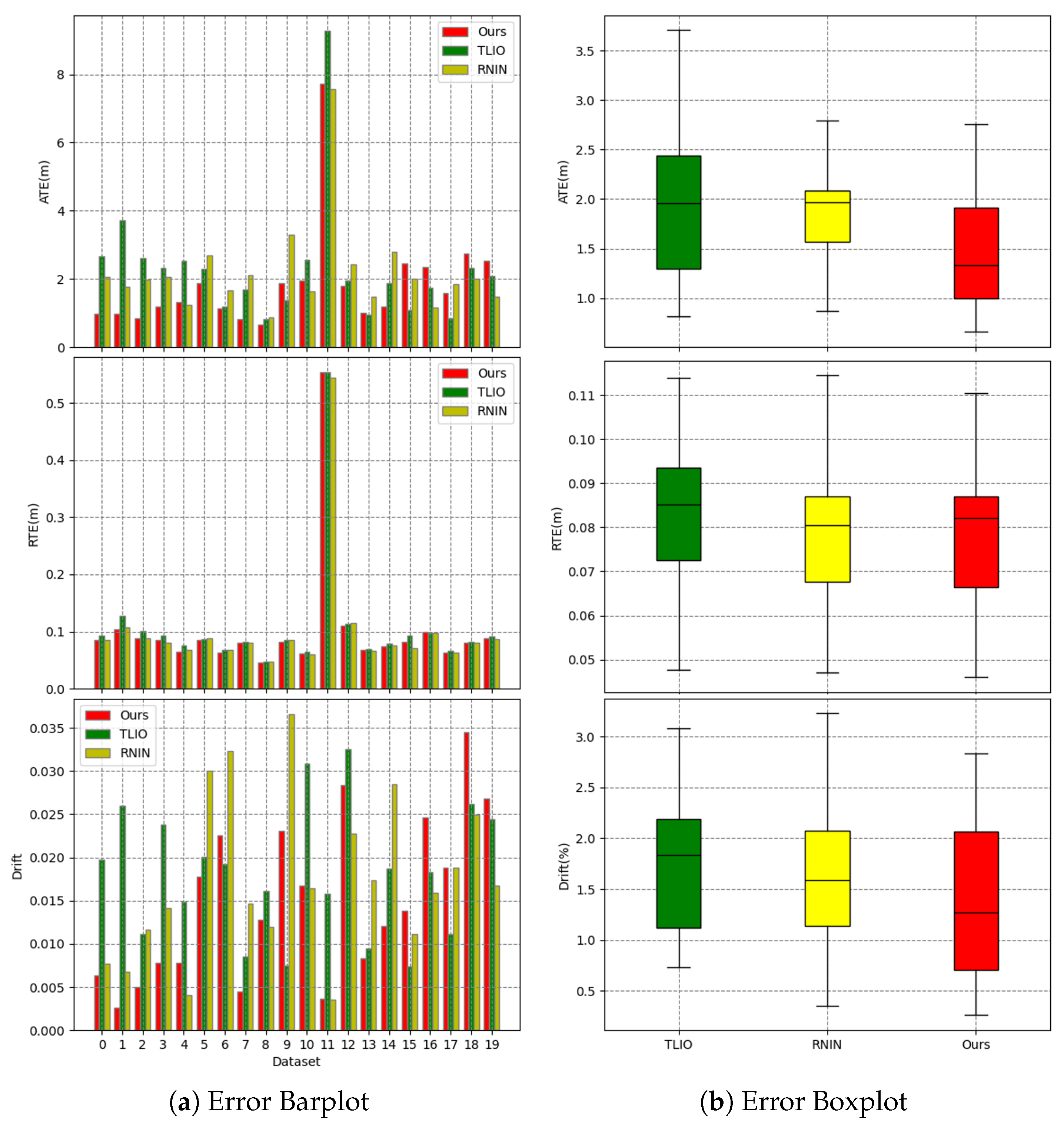
Figure 12.
Error barplot and boxplot. For the barplot, the x-axis represents the dataset, and the y-axis represents the error value. For the boxplot, the x-axis represents the method, and the y-axis represents the error value. The boxplot shows the median, quartiles, and maximum and minimum values of the error.
Table 2.
The x, y, z error of TLIO, RNIN, and our method on the dataset.
Table 3.
Results of TLIO, RNIN, and our method on the dataset.
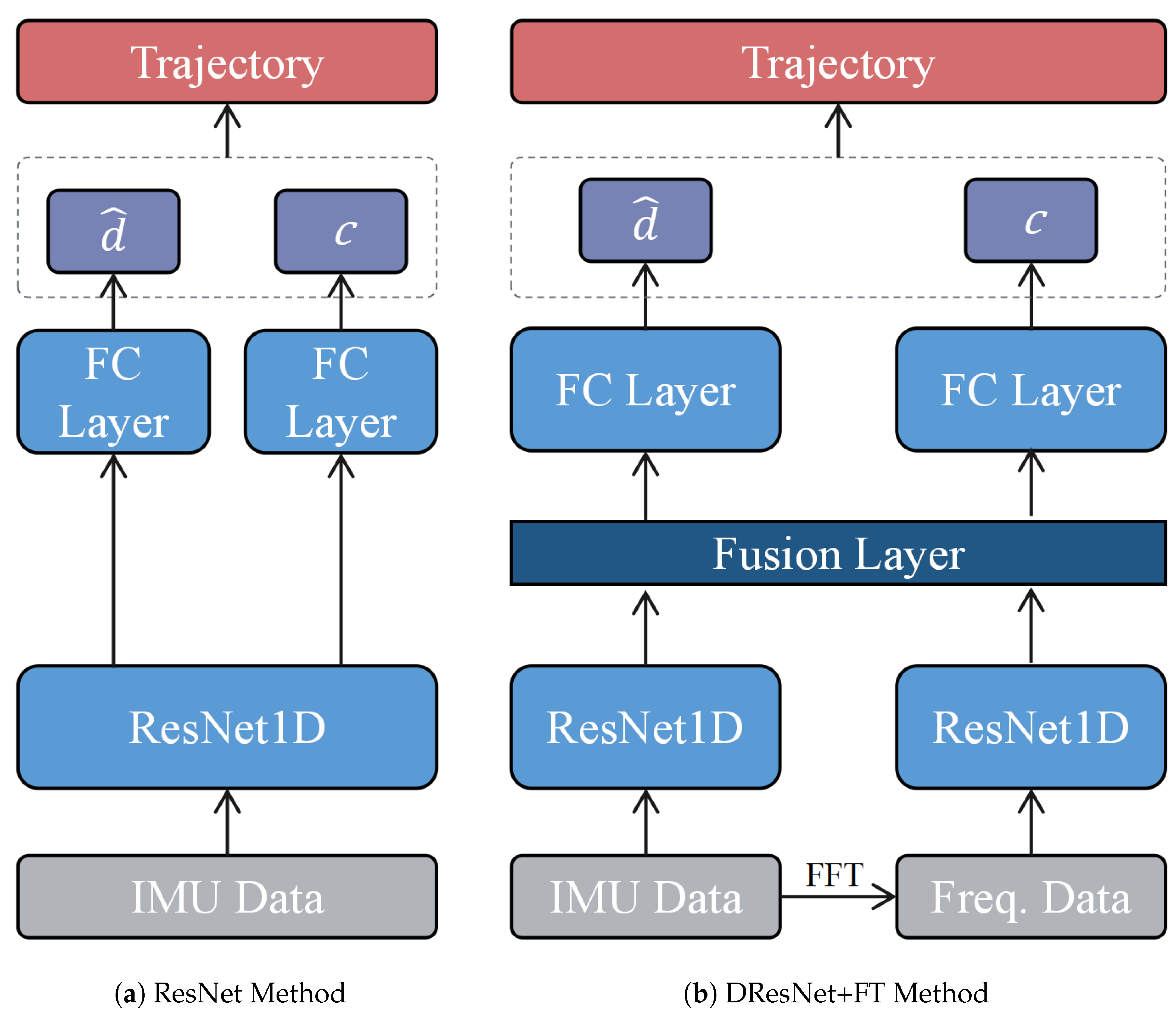
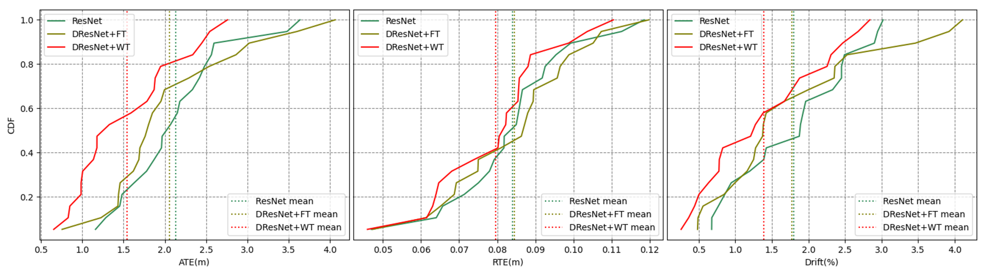
Subsequently, the second series of experiments was formulated with the objective of delineating the influence of frequency-domain analytical tools on the efficacy of spatial positioning algorithms. To this end, we devised comparative experiments for three distinct algorithms, all predicated on the ResNet18 framework to maintain consistency and to mitigate the potential confounding effects of varying network architectures on performance. The algorithms under consideration encompassed a singular ResNet model, a dual ResNet model conjoined with a Fourier transformation, and a dual ResNet model conjoined with a wavelet transformation. The architecture of the other two methods is depicted in Figure 13. The results from these experiments are encapsulated in Figure 14 and Figure 15 and Table 4.
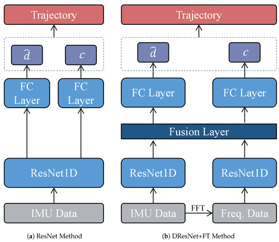
Figure 13.
Architecture of the other two methods.
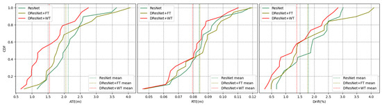
Figure 14.
Error accumulation curves. The x-axis represents the error value, the y-axis represents the cumulative distribution, and the color represents the method.
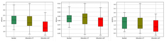
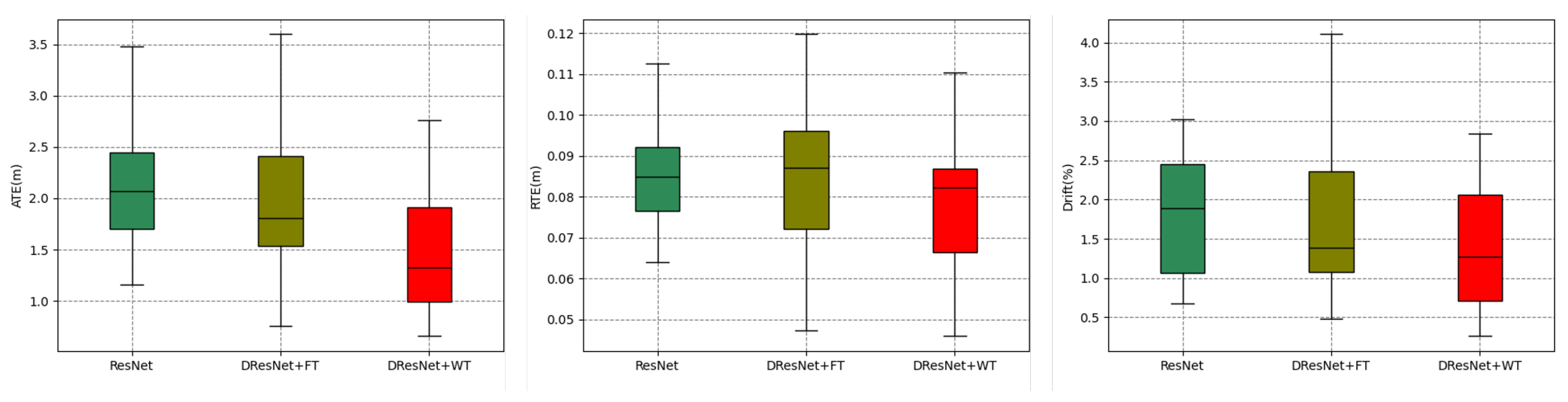
Figure 15.
Error boxplots. The x-axis represents the method, and the y-axis represents the error value.
Table 4.
Results of different methods on the dataset.
5. Discussion
Figure 7 displays the trajectories estimated using our method and the two baseline methods, TLIO and RNIN. We selected six typical results with good, average, and poor prediction performance. Our method’s estimated trajectories were closer to the ground-truth trajectories in most cases compared to the other two methods.
Figure 8 illustrates the three-dimensional errors of the three methods on a test set of 20 trajectories, while Table 2 calculates the average errors in the x, y, and z axes directions. It can be observed that our method exhibited an overall smaller three-dimensional error compared to the other two methods. However, it is noteworthy that there were differences in the error values along the x, y, and z axes, with the z-axis error being significantly smaller than those of the x and y axes. Consequently, in Figure 9, we visualized the three-dimensional error of a representative trajectory, which indeed showed a noticeably smaller error along the z-axis. Considering that during data collection, our equipment typically moved over a larger range in the plane of the x and y axes, and a smaller range along the z-axis (which was usually close to the direction of gravity), taking into account the potential cumulative effect of errors, this difference in error may be related to the range of motion in the respective directions. Figure 10 displays the correlation between three-dimensional error and the range of motion, where we used the Pearson correlation coefficient to calculate the correlation. The greater the positive correlation, the more pronounced the cumulative effect of the error. We used the p-value to judge whether the correlation was significant (a p-value less than 0.05 indicated significant correlation). The results showed that the correlation between error and the range of motion was not significant, indicating that the error of our algorithm did not exhibit a noticeable cumulative effect as the range of motion increased, which demonstrated the advantage of our algorithm over traditional preintegration algorithms. Additionally, we can also see that the performance of our algorithm had a certain positive correlation with the correlation coefficient. In the x, y, and z directions, the smaller the correlation (the weaker the cumulative effect of the error), the better the performance of our algorithm compared to the TLIO and RNIN algorithms, which indirectly reflected that our algorithm had a lesser cumulative effect of error.
Figure 11 shows the overall error cumulative distribution curves of the three methods across 20 test trajectories. Our method exhibited a lower mean error and smaller error extremes for the ATE metric. For the RTE metric, our algorithm performed slightly better than the RNIN algorithm and outperformed the TLIO algorithm. Regarding the drift metric, our method had a lower mean error and maximum error compared to both baseline methods. Overall, in terms of the overall error cumulative distribution test results, our method outperformed the RNIN and TLIO methods. Figure 12a shows the specific errors and overall error situations of the three methods across 20 test trajectories. From the bar chart, we can see the error situation for each test trajectory, and our method demonstrated better results in most cases. Figure 12b reveals that for the ATE metric, our method had the lowest median error, error extremes, and error quartiles. For the RTE metric, our median error was slightly higher than that of the RNIN method, while our error quartiles were slightly lower than those of the RNIN method. For the drift metric, our median error was close to that of the RNIN method, but our error quartiles and error extremes were higher than those of the RNIN method. Therefore, overall, we significantly outperformed the other two methods in the ATE metric, and we were on par with the RNIN method and ahead of the TLIO method for the RTE metric. For the drift metric, our method was close to RNIN and outperformed TLIO. Table 3 encapsulates a comparative analysis of the mean, median, and variance for the ATE, RTE, and drift metrics across a spectrum of 20 test trajectories for the three methodologies under examination. The findings of this analysis revealed that our method secured the superior position in five of the six assessed error metrics, demonstrating its enhanced predictive accuracy. Additionally, our method also achieved the second-best performance in the remaining metric, further substantiating its robustness and efficacy in the domain of inertial spatial positioning.
Figure 14 delineates the aggregate error accumulation distribution curves, and Figure 15 illustrates the error bar plots for the trio of ResNet-based methodologies when applied to the dataset in question. The analysis of the cumulative distribution curves indicated that the neural network spatial positionings, when augmented with tools from the frequency domain, surpassed those of the unadulterated neural network algorithms across the ATE, RTE, and drift metrics. The algorithm integrating a wavelet transformation notably underperformed by a significant margin compared to its counterpart that employed a Fourier transformation. The examination of the box plots suggested that the algorithm predicated on a wavelet transformation yielded diminished errors alongside a more stable and concentrated distribution of error metrics. Table 4 encapsulates the mean and median ATE, RTE, and drift metric values for the trio of ResNet-based algorithms when evaluated against the dataset. The algorithm that incorporated a wavelet transformation secured the optimal outcome across each error metric, while the algorithm utilizing a Fourier transformation attained the second-best results in four out of the six metrics. Conversely, the standalone ResNet algorithm merely secured the second-best outcome in two metrics, with a marginal lead over the third-ranked algorithm.
Upon this comprehensive analysis, the comparative experimental studies conducted with the state-of-the-art TLIO and RNIN algorithms established that the method advanced within this manuscript secured a leading position in terms of accuracy for inertial positioning tasks, with a notable decrease of 20.0% in absolute trajectory error and a significant reduction of 14.6% in relative drift error. Supplementary ablation experiments further corroborated the substantial improvement imparted by the incorporation of frequency-domain methodologies to inertial spatial positioning algorithms. Notably, the wavelet transform approach, which retains the interplay between frequency- and time-domain information, was shown to surpass the efficacy of the Fourier transform method in the context of inertial spatial positioning.
6. Conclusions
This paper proposed a wavelet transform-based neural inertial network for IMU inertial navigation, achieving better performance in spatial positioning compared to advanced algorithms such as TLIO and RNIN. This demonstrates that the time–frequency analysis method based on a wavelet transform can be applied to the design of neural networks, and the combination of time-domain and frequency-domain signals can significantly improve the algorithm’s accuracy and robustness. We adopted a ResNet-based network architecture, which is relatively simple. In the future, increasing the network’s parameter count or introducing new network models could enhance its learning capability. Furthermore, the network design can be further optimized by incorporating new supervision methods and loss functions in the learning of motion features, realizing a two-stage learning architecture for motion patterns and trajectories. The proposed algorithm can be applied to underground robot localization, UAV navigation under GNSS-denied conditions, mixed-reality localization in dark scenarios, and other domains in the future.
Author Contributions
Conceptualization, Y.T. and Y.L.; methodology, Y.T.; software, Y.T.; formal analysis, Y.T.; data curation, Y.T. and Z.Y.; writing—original draft preparation, Y.T.; writing—review and editing, Y.T., J.G., Y.L., G.Z., B.Y. and Z.Y. All authors have read and agreed to the published version of the manuscript.
Funding
This research was funded by the National Key Research and Development Program of China grant number 2020YFF0400403.
Data Availability Statement
The data presented in this study are available on request from the corresponding author. The data are not publicly available due to privacy.
Acknowledgments
We thank all the reviewers and the editors for the insightful comments and suggestions that significantly helped to improve the quality of the paper.
Conflicts of Interest
The authors declare no conflicts of interest. The funders had no role in the design of the study; in the collection, analyses, or interpretation of data; in the writing of the manuscript; or in the decision to publish the results.
References
- Conlin, W.T. Review Paper: Inertial Measurement. arXiv 2017, arXiv:1708.04325. [Google Scholar]
- Zhao, W.; Cheng, Y.; Zhao, S.; Hu, X.; Rong, Y.; Duan, J.; Chen, J. Navigation Grade MEMS IMU for A Satellite. Micromachines 2021, 12, 151. [Google Scholar] [CrossRef] [PubMed]
- White, A.M.; Gardner, W.P.; Borsa, A.A.; Argus, D.F.; Martens, H.R. A Review of GNSS/GPS in Hydrogeodesy: Hydrologic Loading Applications and Their Implications for Water Resource Research. Water Resour. Res. 2022, 58, e2022WR032078. [Google Scholar] [CrossRef]
- Gyagenda, N.; Hatilima, J.V.; Roth, H.; Zhmud, V. A review of GNSS-independent UAV navigation techniques. Robot. Auton. Syst. 2022, 152, 104069. [Google Scholar] [CrossRef]
- Huang, G. Visual-Inertial Navigation: A Concise Review. arXiv 2019, arXiv:1906.02650. [Google Scholar]
- Servières, M.; Renaudin, V.; Dupuis, A.; Antigny, N. Visual and Visual-Inertial SLAM: State of the Art, Classification, and Experimental Benchmarking. J. Sens. 2021, 2021, 1–26. [Google Scholar] [CrossRef]
- European Commission; Joint Research Centre. Assessing Alternative Positioning, Navigation, and Timing Technologies for Potential Deployment in the EU; European Commission: Luxembourg, 2023. [Google Scholar]
- Qin, T.; Li, P.; Shen, S. VINS-Mono: A Robust and Versatile Monocular Visual-Inertial State Estimator. IEEE Trans. Robot. 2018, 34, 1004–1020. [Google Scholar] [CrossRef]
- Campos, C.; Elvira, R.; Rodriguez, J.J.G.; Montiel, J.M.; Tardos, J.D. ORB-SLAM3: An Accurate Open-Source Library for Visual, Visual–Inertial, and Multimap SLAM. IEEE Trans. Robot. 2021, 37, 1874–1890. [Google Scholar] [CrossRef]
- Qin, T.; Pan, J.; Cao, S.; Shen, S. A General Optimization-based Framework for Local Odometry Estimation with Multiple Sensors. arXiv 2019, arXiv:1901.03638. [Google Scholar]
- Bloesch, M.; Omari, S.; Hutter, M.; Siegwart, R. Robust visual inertial odometry using a direct EKF-based approach. In Proceedings of the 2015 IEEE/RSJ International Conference on Intelligent Robots and Systems (IROS), Hamburg, Germany, 28 September–3 October 2015; pp. 298–304. [Google Scholar] [CrossRef]
- Gao, G.; Gao, B.; Gao, S.; Hu, G.; Zhong, Y. A Hypothesis Test-Constrained Robust Kalman Filter for INS/GNSS Integration With Abnormal Measurement. IEEE Trans. Veh. Technol. 2023, 72, 1662–1673. [Google Scholar] [CrossRef]
- Gao, B.; Hu, G.; Zhu, X.; Zhong, Y. A Robust Cubature Kalman Filter with Abnormal Observations Identification Using the Mahalanobis Distance Criterion for Vehicular INS/GNSS Integration. Sensors 2019, 19, 5149. [Google Scholar] [CrossRef] [PubMed]
- Hu, G.; Gao, B.; Zhong, Y.; Ni, L.; Gu, C. Robust Unscented Kalman Filtering With Measurement Error Detection for Tightly Coupled INS/GNSS Integration in Hypersonic Vehicle Navigation. IEEE Access 2019, 7, 151409–151421. [Google Scholar] [CrossRef]
- Wu, X.; Xiao, B.; Wu, C.; Guo, Y.; Li, L. Factor graph based navigation and positioning for control system design: A review. Chin. J. Aeronaut. 2022, 35, 25–39. [Google Scholar] [CrossRef]
- Beuchert, J.; Camurri, M.; Fallon, M. Factor Graph Fusion of Raw GNSS Sensing with IMU and Lidar for Precise Robot Localization without a Base Station. arXiv 2023, arXiv:2209.14649. [Google Scholar]
- Lyu, P.; Wang, B.; Lai, J.; Bai, S.; Liu, M.; Yu, W. A Factor Graph Optimization Method for High-Precision IMU-Based Navigation System. IEEE Trans. Instrum. Meas. 2023, 72, 9509712. [Google Scholar] [CrossRef]
- Gao, B.; Gao, S.; Zhong, Y.; Hu, G.; Gu, C. Interacting multiple model estimation-based adaptive robust unscented Kalman filter. Int. J. Control. Autom. Syst. 2017, 15, 2013–2025. [Google Scholar] [CrossRef]
- Gao, B.; Hu, G.; Zhong, Y.; Zhu, X. Cubature Kalman Filter With Both Adaptability and Robustness for Tightly-Coupled GNSS/INS Integration. IEEE Sens. J. 2021, 21, 14997–15011. [Google Scholar] [CrossRef]
- Chen, C.; Lu, X.; Markham, A.; Trigoni, N. IONet: Learning to Cure the Curse of Drift in Inertial Odometry. Proc. AAAI Conf. Artif. Intell. 2018, 32, 6468–6476. [Google Scholar] [CrossRef]
- Kang, W.; Han, Y. SmartPDR: Smartphone-Based Pedestrian Dead Reckoning for Indoor Localization. IEEE Sens. J. 2015, 15, 2906–2916. [Google Scholar] [CrossRef]
- Foxlin, E. Pedestrian Tracking with Shoe-Mounted Inertial Sensors. IEEE Comput. Graph. Appl. 2005, 25, 38–46. [Google Scholar] [CrossRef]
- Brajdic, A.; Harle, R. Walk detection and step counting on unconstrained smartphones. In Proceedings of the 2013 ACM International Joint Conference on Pervasive and Ubiquitous Computing, Zurich, Switzerland, 8–12 September 2013; pp. 225–234. [Google Scholar] [CrossRef]
- Yan, H.; Shan, Q.; Furukawa, Y. RIDI: Robust IMU Double Integration. In Computer Vision—ECCV 2018; Ferrari, V., Hebert, M., Sminchisescu, C., Weiss, Y., Eds.; Series Title: Lecture Notes in Computer Science; Springer International Publishing: Cham, Switzerland, 2018; Volume 11217, pp. 641–656. [Google Scholar] [CrossRef]
- Herath, S.; Yan, H.; Furukawa, Y. RoNIN: Robust Neural Inertial Navigation in the Wild: Benchmark, Evaluations, & New Methods. In Proceedings of the 2020 IEEE International Conference on Robotics and Automation (ICRA), Virtual, 31 May–31 August 2020; pp. 3146–3152, ISSN 2577-087X. [Google Scholar] [CrossRef]
- Liu, W.; Caruso, D.; Ilg, E.; Dong, J.; Mourikis, A.I.; Daniilidis, K.; Kumar, V.; Engel, J. TLIO: Tight Learned Inertial Odometry. IEEE Robot. Autom. Lett. 2020, 5, 5653–5660. [Google Scholar] [CrossRef]
- Chen, D.; Wang, N.; Xu, R.; Xie, W.; Bao, H.; Zhang, G. RNIN-VIO: Robust Neural Inertial Navigation Aided Visual-Inertial Odometry in Challenging Scenes. In Proceedings of the 2021 IEEE International Symposium on Mixed and Augmented Reality (ISMAR), Bari, Italy, 4–8 October 2021; pp. 275–283. [Google Scholar] [CrossRef]
- Sun, S.; Melamed, D.; Kitani, K. IDOL: Inertial Deep Orientation-Estimation and Localization. Proc. AAAI Conf. Artif. Intell. 2021, 35, 6128–6137. [Google Scholar] [CrossRef]
- Hou, X.; Bergmann, J.H. HINNet: Inertial navigation with head-mounted sensors using a neural network. Eng. Appl. Artif. Intell. 2023, 123, 106066. [Google Scholar] [CrossRef]
- Mao, Y.; Zhong, Y.; Gao, Y.; Wang, Y. A Weak SNR Signal Extraction Method for Near-Bit Attitude Parameters Based on DWT. Actuators 2022, 11, 323. [Google Scholar] [CrossRef]
- Severin, I.C.; Dobrea, D.M. 6DOF Inertial IMU Head Gesture Detection: Performance Analysis Using Fourier Transform and Jerk-Based Feature Extraction. In Proceedings of the 2020 IEEE Microwave Theory and Techniques in Wireless Communications (MTTW), Riga, Latvia, 1–2 October 2020; Volume 1, pp. 118–123. [Google Scholar] [CrossRef]
- Xu, W.; Cai, Y.; He, D.; Lin, J.; Zhang, F. FAST-LIO2: Fast Direct LiDAR-Inertial Odometry. IEEE Trans. Robot. 2022, 38, 2053–2073. [Google Scholar] [CrossRef]


Disclaimer/Publisher’s Note: The statements, opinions and data contained in all publications are solely those of the individual author(s) and contributor(s) and not of MDPI and/or the editor(s). MDPI and/or the editor(s) disclaim responsibility for any injury to people or property resulting from any ideas, methods, instructions or products referred to in the content. |
© 2024 by the authors. Licensee MDPI, Basel, Switzerland. This article is an open access article distributed under the terms and conditions of the Creative Commons Attribution (CC BY) license (https://creativecommons.org/licenses/by/4.0/).