Point Cloud Denoising in Outdoor Real-World Scenes Based on Measurable Segmentation

Abstract

With the continuous advancements in three-dimensional scanning technology, point clouds are fundamental data in various fields such as autonomous driving, 3D urban modeling, and the preservation of cultural heritage. However, inherent inaccuracies in instruments and external environmental interference often introduce noise and outliers into point cloud data, posing numerous challenges for advanced processing tasks such as registration, segmentation, classification, and 3D reconstruction. To effectively address these issues, this study proposes a hierarchical denoising strategy based on finite measurable segmentation in spherical space, taking into account the performance differences in horizontal and vertical resolutions of LiDAR systems. The effectiveness of this method was validated through a denoising experiment conducted on point cloud data collected from real outdoor environments. The experimental result indicates that this denoising strategy not only effectively eliminates noise but also more accurately preserves the original detail features of the point clouds, demonstrating significant advantages over conventional denoising techniques. Overall, this study introduces a novel and effective method for denoising point cloud data in outdoor real-world scenes.

1. Introduction

With the rapid advancement of three-dimensional sensing technologies, point cloud data have become an indispensable component in various applications [1]. From the 3D reconstruction of ancient ruins to contemporary autonomous vehicles, point clouds offer an intuitive and precise representation of three-dimensional data. This superior form of data representation has found extensive applications in virtual reality [2,3,4], augmented reality [5,6], autonomous vehicles [7,8,9], geological surveys [10,11,12,13], and many other domains. However, due to the inherent limitations of 3D scanning and sensing technologies, coupled with environmental noise, scattering, refraction, and other interference factors, the use of point cloud data often comes with significant noise and outliers.

Such noise and outliers pose substantial challenges to further processing point cloud data [14]. For instance, in point cloud registration tasks, noise and outliers can lead to incorrect registration results, subsequently affecting the accuracy of the entire 3D model. For feature extraction and object recognition tasks, noise and outliers can obscure features, leading to misidentification [15]. Thus, denoising point clouds is a crucial step in any point cloud processing pipeline [16]. Effective denoising not only enhances data quality but also establishes a more robust foundation for subsequent processing steps. However, it is worth noting that the diversity of point cloud data implies there is not a singular denoising strategy suitable for all applications. Different applications and scenes often demand specific treatments and optimizations.

Over the past few years, researchers have made some progress in terms of outlining point cloud denoising methods. Cheng et al. [17] proposed a denoising algorithm based on mesh principal component analysis and ground splicing that effectively removes noise from point cloud data. However, this method may lose features of objects outside the plane while removing noise and requires precise parameter adjustment to achieve the best denoising effect. Sun et al. [18] proposed a structure-aware denoising method for real-world noisy point clouds, effectively preserving point cloud structures while removing noise by combining external and internal prior knowledge, demonstrating excellent comprehensive performance. Nonetheless, this method may face challenges when dealing with specific complex structures in point clouds. Zheng et al. [19] proposed a single-stage adaptive multi-scale point cloud noise filtering algorithm based on feature information, which, through an efficient kd-tree structure and improved normal vector estimation method, can quickly and accurately process both large-scale and small-scale noise while maintaining the geometric features of the point cloud. Despite its effectiveness, this algorithm involves multiple parameters, is sensitive to parameter settings, and has a high level of computational complexity, which results in longer processing times for large point clouds. Shi et al. [20] proposed a three-dimensional point cloud denoising algorithm based on a gravitational feature function. This algorithm effectively removes sparse and dense drift noises in point cloud data by calculating the gravitational force between the centroid of the point cloud and the spherical neighborhood of points. However, this method may incorrectly identify small objects in scenes with large size differences as noise, indicating limitations in specific application scenarios. Charron et al. [21] proposed a dynamic radius outlier removal (DROR) filter, considering the changing point cloud density with increasing distance from the sensor, to effectively remove noise caused by snow while retaining scene details. Even so, this method faces challenges in processing points close to the sensor and avoiding the erroneous deletion of non-snow points, requiring careful adjustment of parameters to adapt to different scenes. Nevertheless, a common challenge faced by these methods is how to balance denoising performance and computational efficiency. Processing large-scale, high-density point cloud data requires substantial computational resources and time, which is unacceptable in some real-time applications. Furthermore, excessive denoising may lead to the loss of important information within the data, thus diminishing the representational ability of the point cloud. Therefore, ensuring both denoising performance and computational efficiency while maintaining data quality is crucial.

To address these challenges, this study introduces an innovative hierarchical denoising method that leverages the high resolution of LiDAR in the horizontal direction and the low resolution in the vertical direction. This method decomposes point cloud data into multiple subsets, allowing for the selection of suitable denoising parameters for different spatial regions of the point cloud subsets, thereby enabling precise control over noise and outliers.

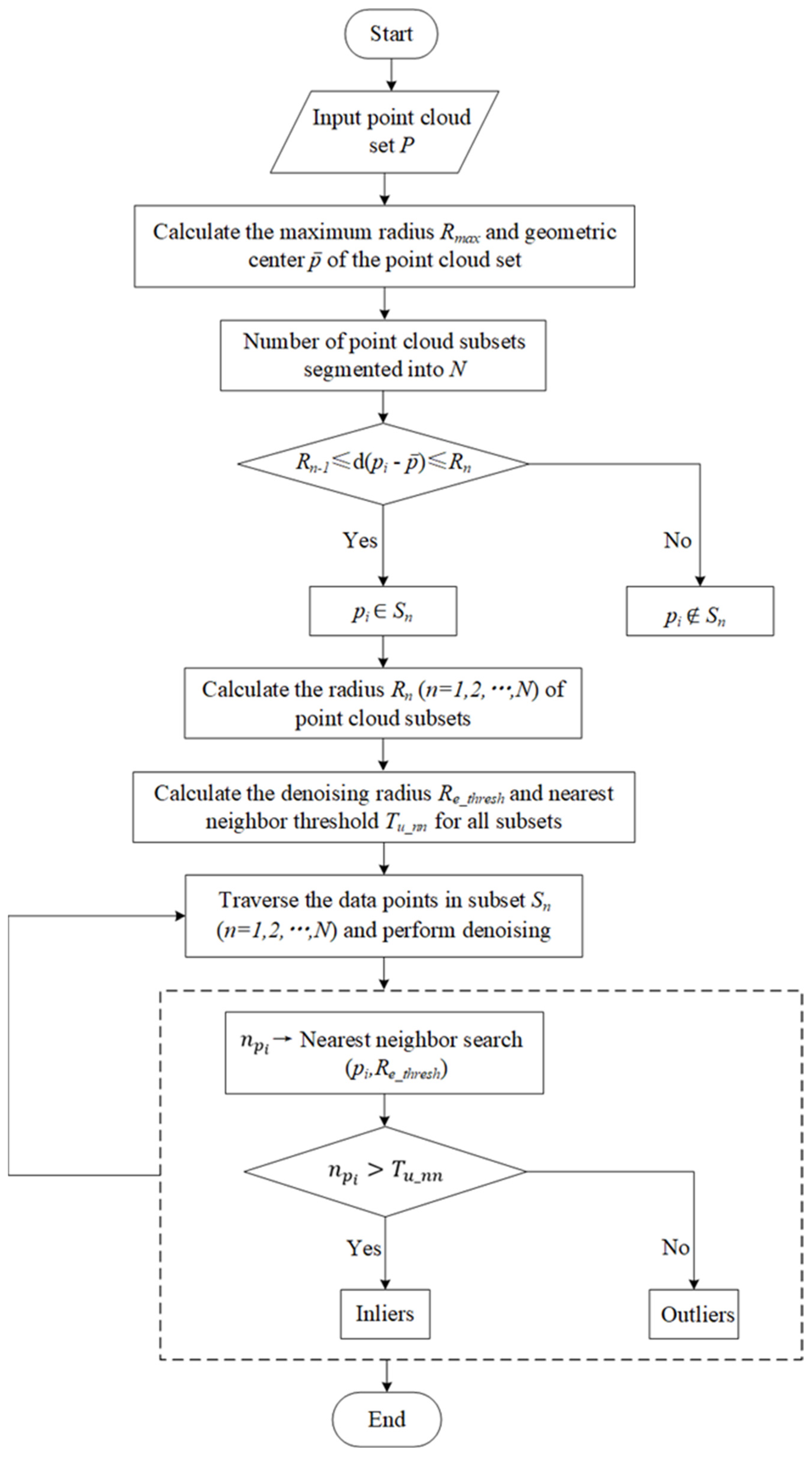
2. Methodology

2.1. Calculation of the Maximum Radius

The maximum radius of a point cloud is the radius of a sphere surrounding the entire point cloud. For a point cloud composed of $n$ points, the calculation formula for the maximum radius $R_{\max }$ is as follows:

$$R_{\max }={\max }_{i=1,2,\dots ,n}d(p_i-\overline{p})$$

(1)

where $\overline{p}$ is the mean value of $p_i$ and the center of the point cloud.

2.2. Calculation of the Number of Concentric Spheres

To compute the number of concentric spheres under the framework of spherical space finite measurable segmentation, the maximum bounding sphere for the entire point cloud is constructed based on the calculated maximum radius $R_{\max }$. Subsequently, the number of concentric spheres (number of point cloud subsets) is determined using the obtained maximum radius $R_{\max }$. The specific formula for calculating the number of concentric spheres $N$ is as follows:

$$N=\lambda ⌈\sqrt{R_{\max }}⌉$$

(2)

where $\lambda$ represents an adjustment coefficient and $⌈\cdot ⌉$ represents the ceiling function.

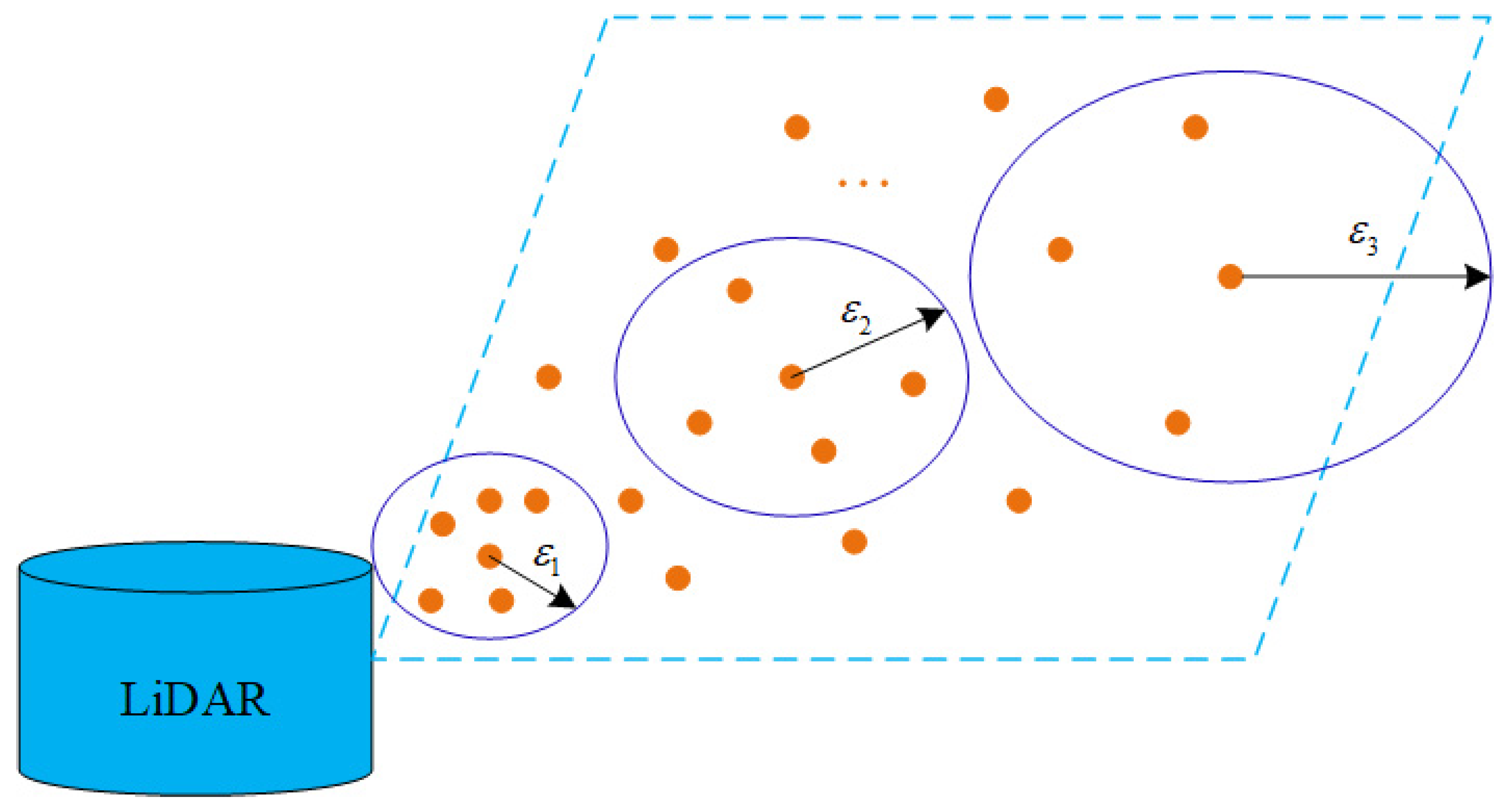
2.3. Finite Measurable Segmentation of Point Clouds in Spherical Space

2.3.1. Equidistant Segmentation (ES) and Proportional Segmentation (PS)

Assuming the outermost bounding sphere of the entire point cloud constitutes a measurable space $\left(X,\mathcal{F}\right)$, when this measurable space is subjected to equidistant and proportional finite measurable segmentation, the spherical space is partitioned into a series of concentric spheres denoted as $S_n, n=1,2,\dots ,N$ with a property $S_n\in \mathcal{F}$. The radius of the concentric spheres generated under these two segmentation methods differ, resulting in varied distributions of the point cloud at different hierarchies within the spherical space. Equidistant segmentation divides the spherical space surrounding the entire point cloud into several subsets $S_n$ with equal differences in the radii of adjacent subsets. Proportional segmentation divides the spherical space surrounding the entire point cloud into several subsets $S_n$ with an equal ratio of radii of adjacent subsets. The radius $R_n$ corresponding to the subset $S_n$ is calculated as follows:

$$R_n=\left\{\begin{array}{c}n(\frac{R_{\max }}{N}); \mathrm{ES}\\ D\sqrt[N]{{\left(\frac{R_{\max }}{D}\right)}^n}; \mathrm{PS} \end{array}\right.(n=1,2,\dots ,N)$$

(3)

where $n$ represents the sequence number of point cloud subsets under equidistant and proportional segmentations in the spherical space. $D$ represents the detection blind area of the LiDAR, and the formula for calculating the blind area range is as follows:

$$D=h\tan (\frac{\pi }{2}-{\theta }_v)$$

(4)

where $h$ represents the installation height of the LiDAR and ${\theta }_v$ represents the vertical field angle of view of the LiDAR.

For any point $p_i$ in the point cloud, if the distance to the center $\overline{p}$ of the point cloud satisfies the following formula:

$$R_{n-1}\le d(p_i,\overline{p})\le R_n, n=1,2,\dots ,N$$

(5)

then $p_i$ is a part of the subset $S_n$. Both equidistant and proportional segmentations are employed to ensure the finite measurable segmentation of the point cloud in spherical space.

2.3.2. Distribution of Point Clouds in Different Hierarchical Spaces

The standard deviation (SD) serves as a statistical metric to characterize variability within a dataset. By setting the radii of concentric spheres, the study assesses the segmentation effects of point clouds at various hierarchical levels within spherical spaces. The standard deviation within each hierarchy and the total standard deviation (TSD) were calculated to evaluate the consistency of point cloud distributions across different hierarchies and the entire dataset. At a specific hierarchy, a smaller standard deviation indicates higher uniformity in the point cloud distribution, whereas a larger standard deviation suggests poorer uniformity. The total standard deviation acts as a comprehensive metric for assessing the uniformity of the entire point cloud distribution. Specifically, a smaller total standard deviation indicates that the uniformity of the point cloud distribution is consistent across different hierarchies, while a larger total standard deviation indicates a significant variability in uniformity between hierarchies. The calculation formulas for the standard deviation at different hierarchies ${\sigma }_n$ and the overall standard deviation $\sum$ are as follows:

$${\sigma }_n=\sqrt{\frac{1}{m}{\displaystyle \sum _{i=1}^m{(N{N}_i-\overline{NN})}^2}}$$

(6)

$$\sum =\sqrt{\frac{1}{N-1}{\displaystyle \sum _{n=1}^N{({\sigma }_n-\overline{\sigma })}^2}}$$

(7)

where $m$ represents the number of points in the same hierarchy, $N$ represents the number of point cloud subsets, $N{N}_i$ represents the nearest neighbor distance of point $p_i$ within that hierarchy, $\overline{NN}$ represents the mean value of $N{N}_i$, and $\overline{\sigma }$ represents the mean value of ${\sigma }_n$.

2.4. Calculation of Point Cloud Hierarchical Denoising Parameters

2.4.1. Calculation of Point Cloud Hierarchical Denoising Parameters under Equidistant Segmentation

The spherical space enclosing the point cloud set is divided into finite measurable segments with a fixed radius difference through equidistant segmentation. For a series of subspaces generated by this segmentation, different parameters (radius threshold and neighboring point threshold) are selected to perform adaptive denoising on the point cloud. Among them, the calculation formula of the radius threshold $R_{e\_thresh}$ is as follows:

$$R_{e\_thresh}=M{\delta }_h{R}_n$$

(8)

where $M$ represents the magnification factor, ${\delta }_h$ denotes the theoretical value of the distance between adjacent points in the horizontal direction of the LiDAR, and $R_n$ represents the radius of the concentric sphere under equidistant segmentation, and its detailed expression is shown in Formula (3). The specific calculation formulas for $M$ and ${\delta }_h$ are as follows:

$$M=\frac{V_{\mathrm{deg}}}{2H_{\mathrm{deg}}}$$

(9)

$${\delta }_h=2\sin (\frac{H_{rad}}{2})$$

(10)

where $V_{\mathrm{deg}}$ denotes the vertical resolution of the LiDAR, while $H_{\mathrm{deg}}$ signifies the horizontal resolution of the LiDAR, and $H_{rad}$ represents the horizontal resolution of the LiDAR measured in radians.

In the context of equidistant segmentation in spherical space, the calculation formula for the threshold $T_{u\_nn}$ of neighboring points at different hierarchies is as follows:

$$T_{u\_nn}=⌈\max (5, 10R_{e\_thresh}+1)⌉$$

(11)

To concisely and structurally present the logic and steps of the algorithm for hierarchically denoising point clouds using equidistant segmentation in spherical space, the flowchart of the algorithm is provided in Figure 1.

2.4.2. Calculation of Point Cloud Hierarchical Denoising Parameters under Proportional Segmentation

Compared with the equidistant segmentation with a fixed radius difference, the calculation of adaptive denoising parameters for point clouds under the proportional segmentation with a fixed radius ratio is slightly different. The calculation of the denoising radius threshold $R_{p\_thresh}$ is similar to Formula (8), but the only difference is that the calculation of the radius $R_n$ of the point cloud subset should be based on the proportional segmentation method. The calculation of the magnification factor $M$ and the theoretical value ${\delta }_h$ of the horizontal spacing between adjacent data points per unit distance remain consistent with Formulas (9) and (10), respectively. The process for hierarchical point cloud denoising under proportional segmentation of spherical space is structurally similar to that under equidistant segmentation. The calculation formula for the threshold $T_{p\_nn}$ of neighboring points for denoising point clouds in different hierarchical subspaces under proportional segmentation is as follows:

$$T_{p\_nn}=⌈\max (5, 10\log (1+12R_{p\_thresh})-10⌉$$

(12)

where the functions $\max (\cdot )$ and $⌈\cdot ⌉$ retain their previously defined interpretations.

3. Experiment

3.1. Experimental Setup

3.1.1. Dataset Description

The point cloud dataset used in this study was collected from an outdoor real-world scene using the WLR-720 model LiDAR produced by VanJee Corporation, located in Beijing, China. This device is equipped with 16 scanning beams and has an effective ranging capability of up to 120 m (ranging from 0.5 m to 70 m at 10% reflectivity). It can perform a 360° full-range scan horizontally at a frequency of 20 Hz. Vertically, its field of view is 30°, spanning from −16° to 14°, thus providing extensive coverage of the vertical space. The WLR-720 achieves a resolution of 0.1° horizontally and 2° vertically, with a ranging accuracy of ±2 cm (typical value).

In this experiment, 1,489,400 data points were collected using the LiDAR system in outdoor real-world scenes. The acquired point cloud data comprehensively document the three-dimensional spatial coordinates of each data point, as well as the reflectance information of various targets. The scan encompassed a variety of subjects including buildings, trees, ground surfaces, vehicles, and pedestrians, among others. Figure 2 displays the raw point cloud data collected from the outdoor real-world scenes.

3.1.2. Experimental Environment and Tools

To verify the effectiveness of the point cloud denoising method proposed in this study, relevant experiments were conducted within specific hardware and software settings. The configuration of the experimental platform is as follows:

(1)

Hardware environment

• CPU: High-performance Intel^® Core™ i9-14900 with a clock speed of up to 5.8 GHz, providing robust data processing capabilities.
• Graphics Card: NVIDIA^® GeForce RTX™ 4060, supports efficient graphical processing.
• Memory: 32 GB of Samsung DDR5, ensuring ample data processing and storage capacity.

(2)

Software environment

The experiments were performed on a Windows 10 operating system. Data processing and analysis primarily relied on the Python 3.8.8 environment and its associated scientific computing libraries. The tools used included the Spyder 5.4.3 integrated development environment, Pandas 1.4.3 and NumPy 1.22.0 for data processing, SciPy 1.7.3 for scientific calculations, and Open3D 0.13.0 for visualization and processing of point cloud datasets.

3.2. Experimental Result

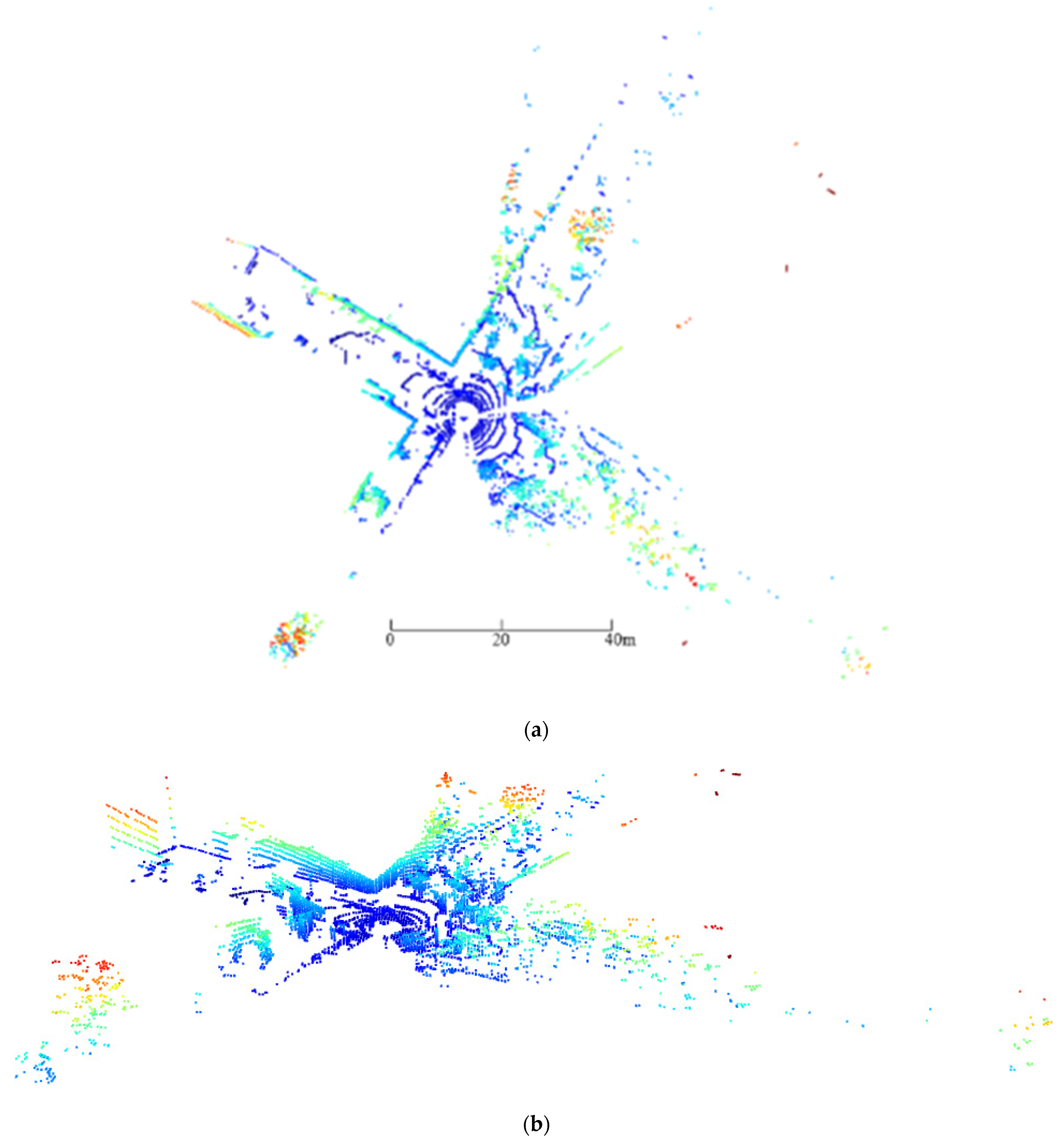
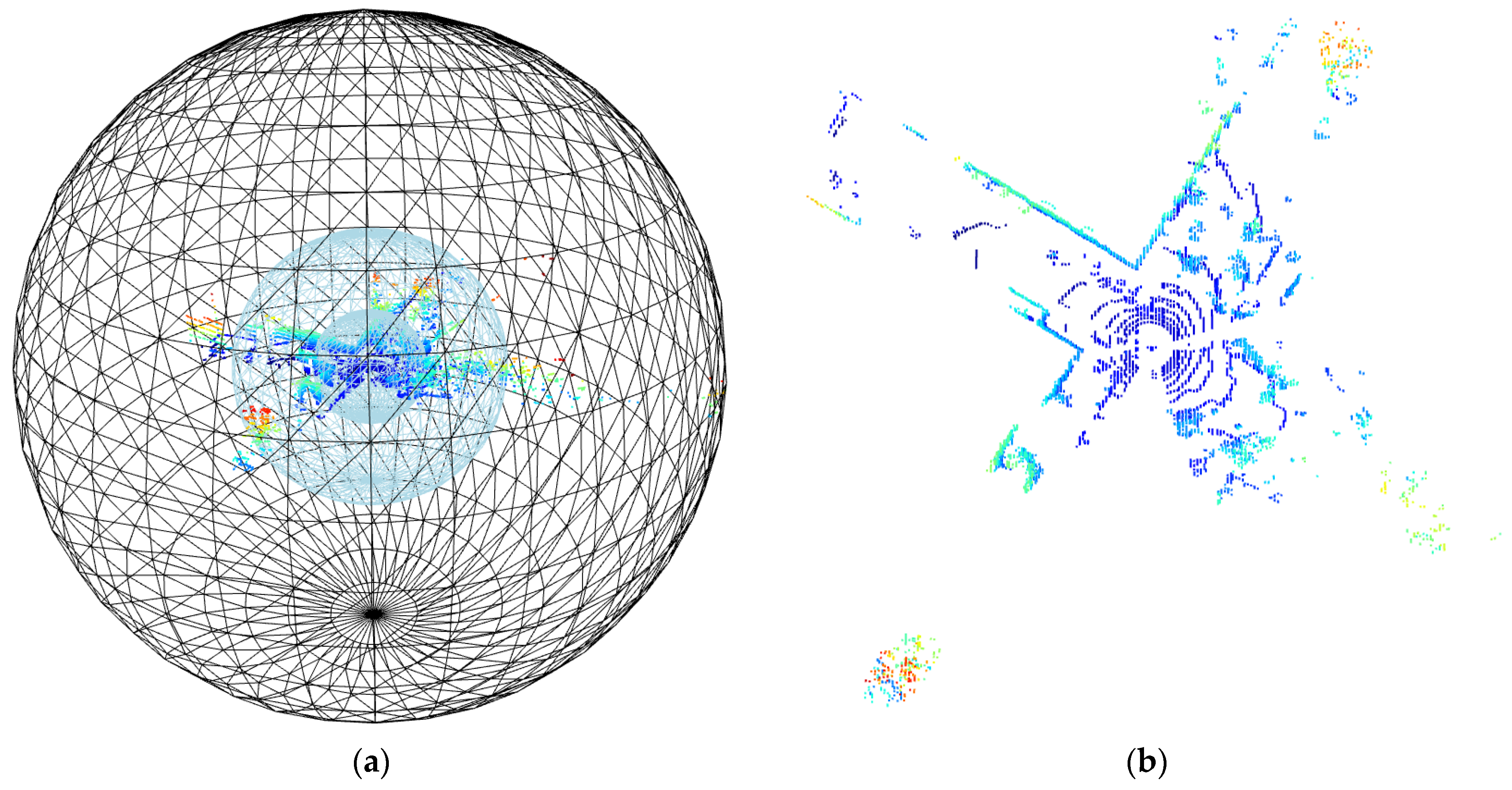
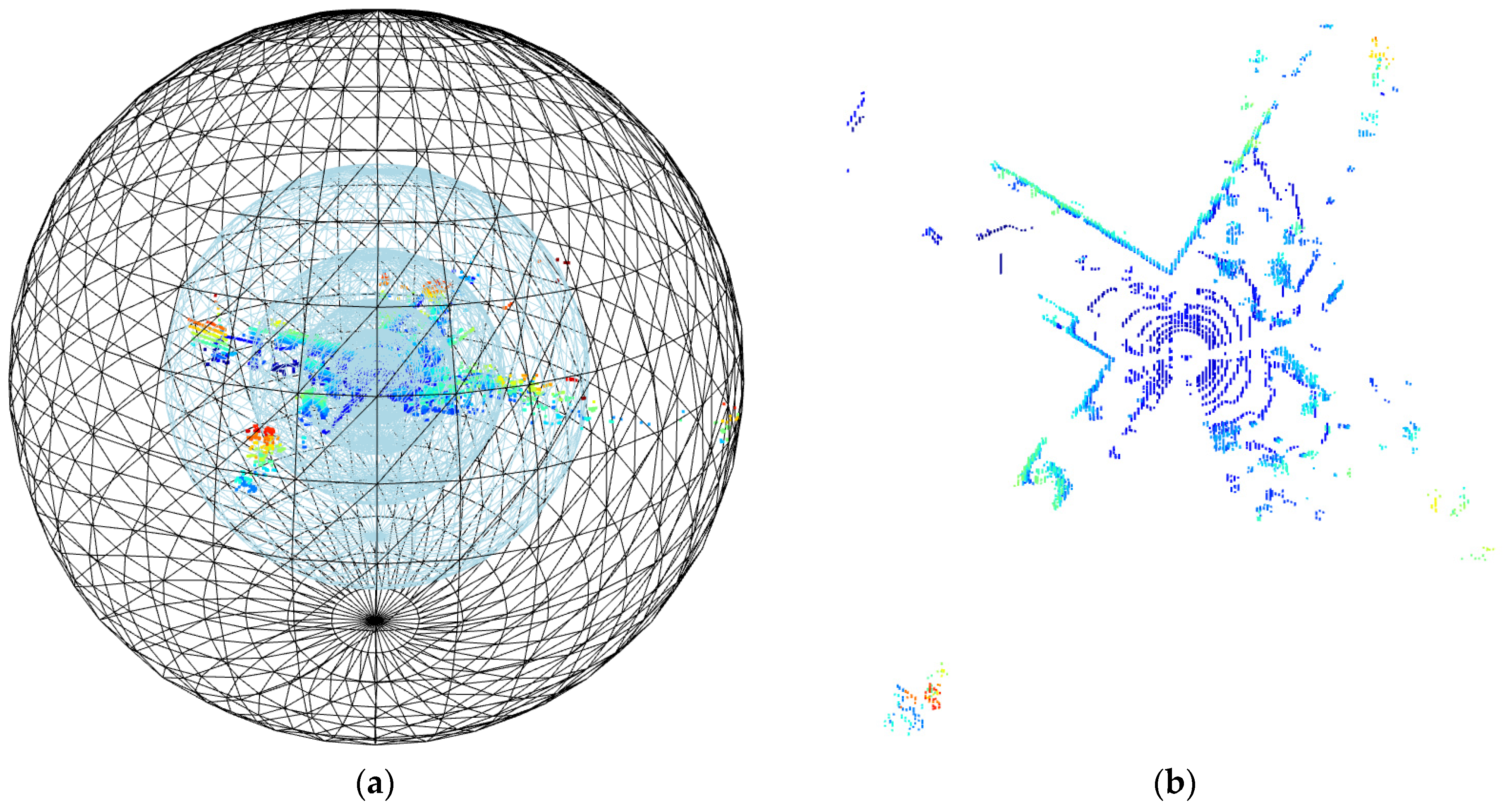
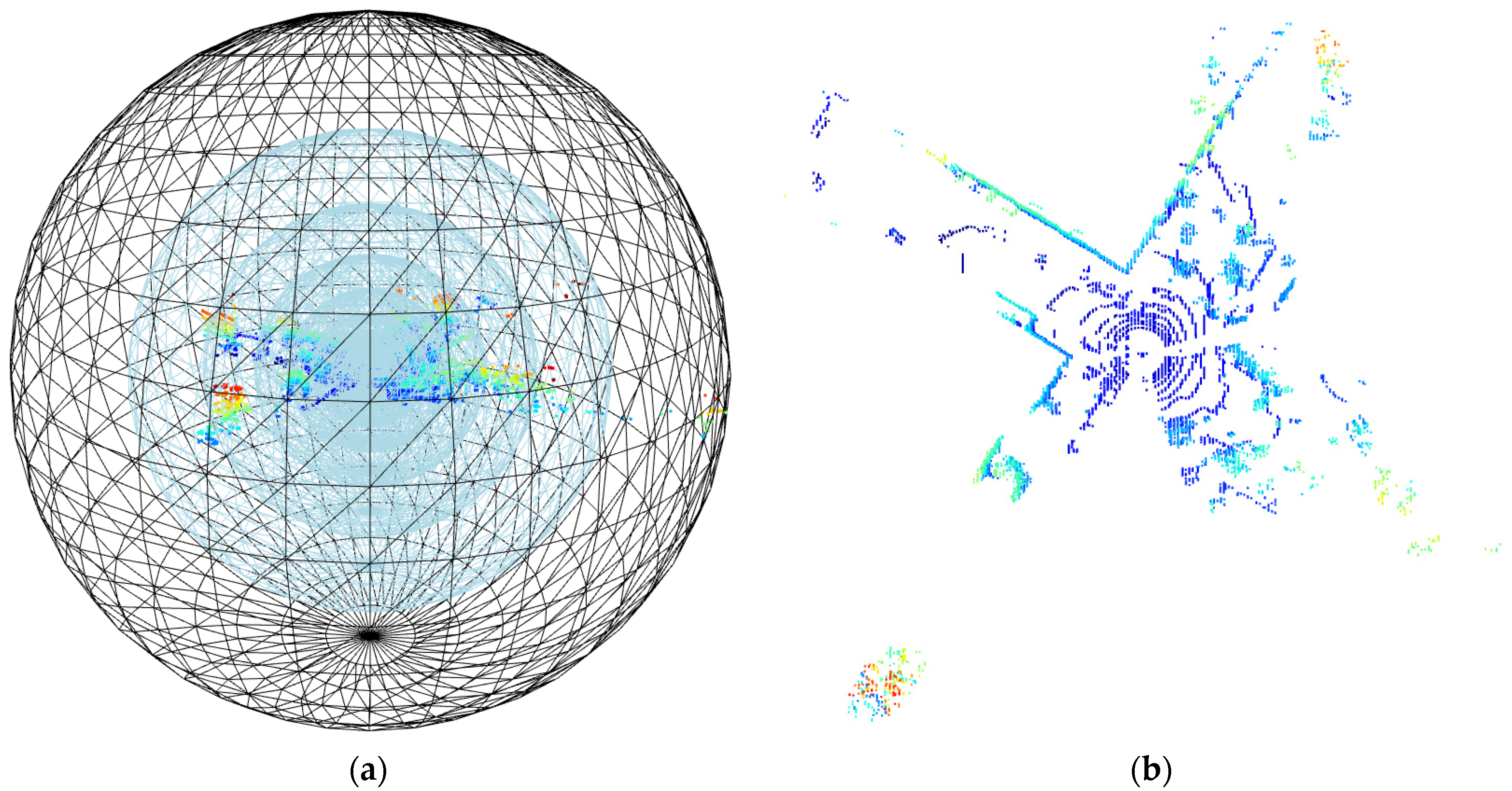
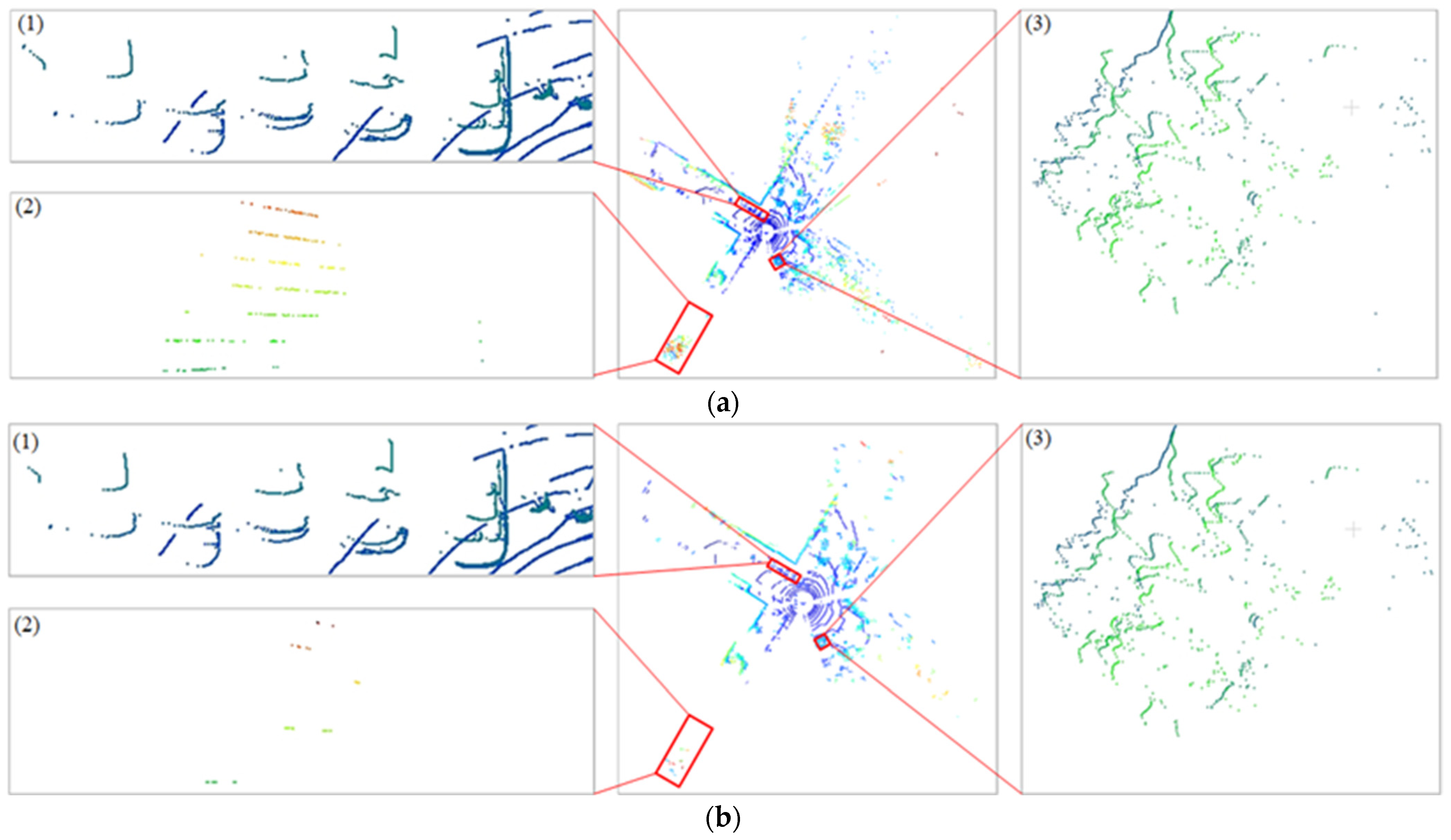
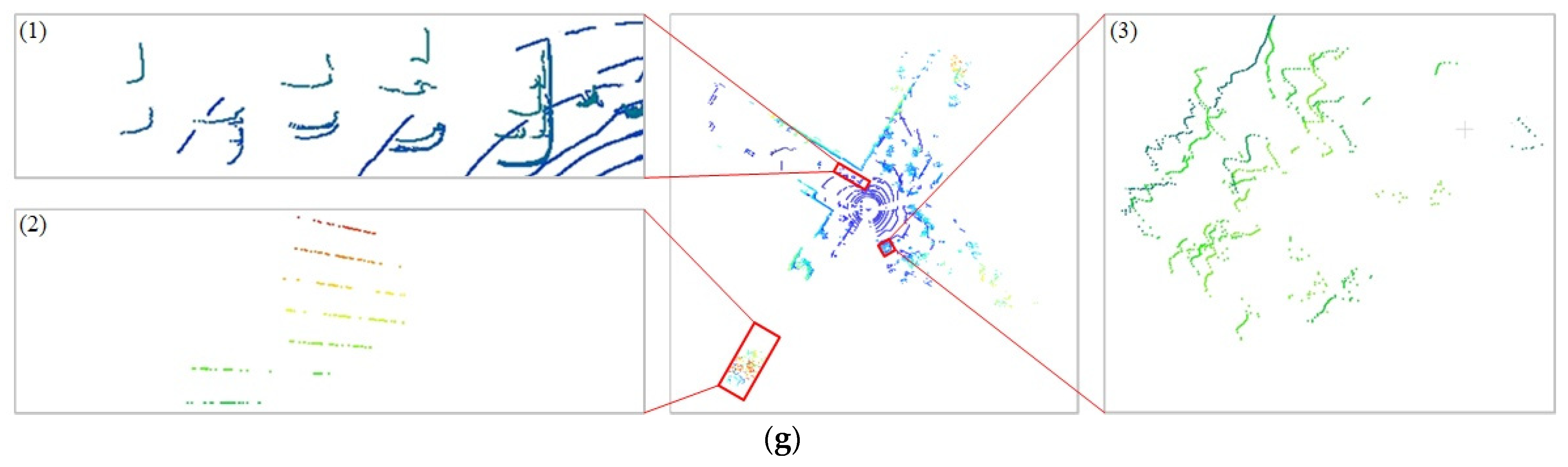
3.2.1. Visualization Comparison of Point Cloud before and after Hierarchical Denoising

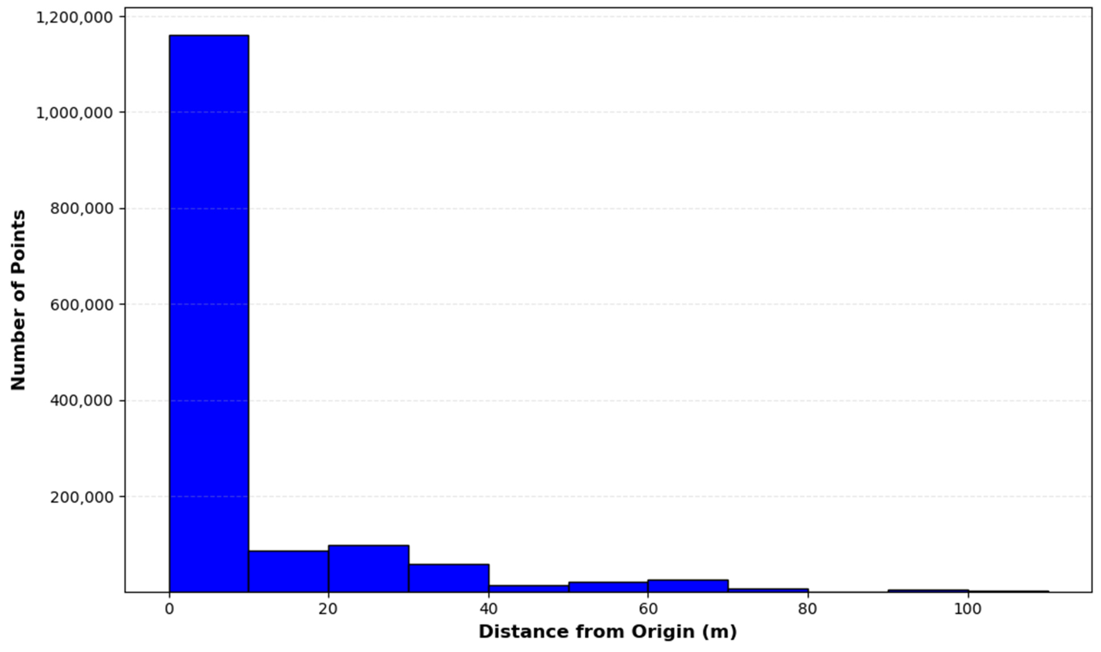
(1)

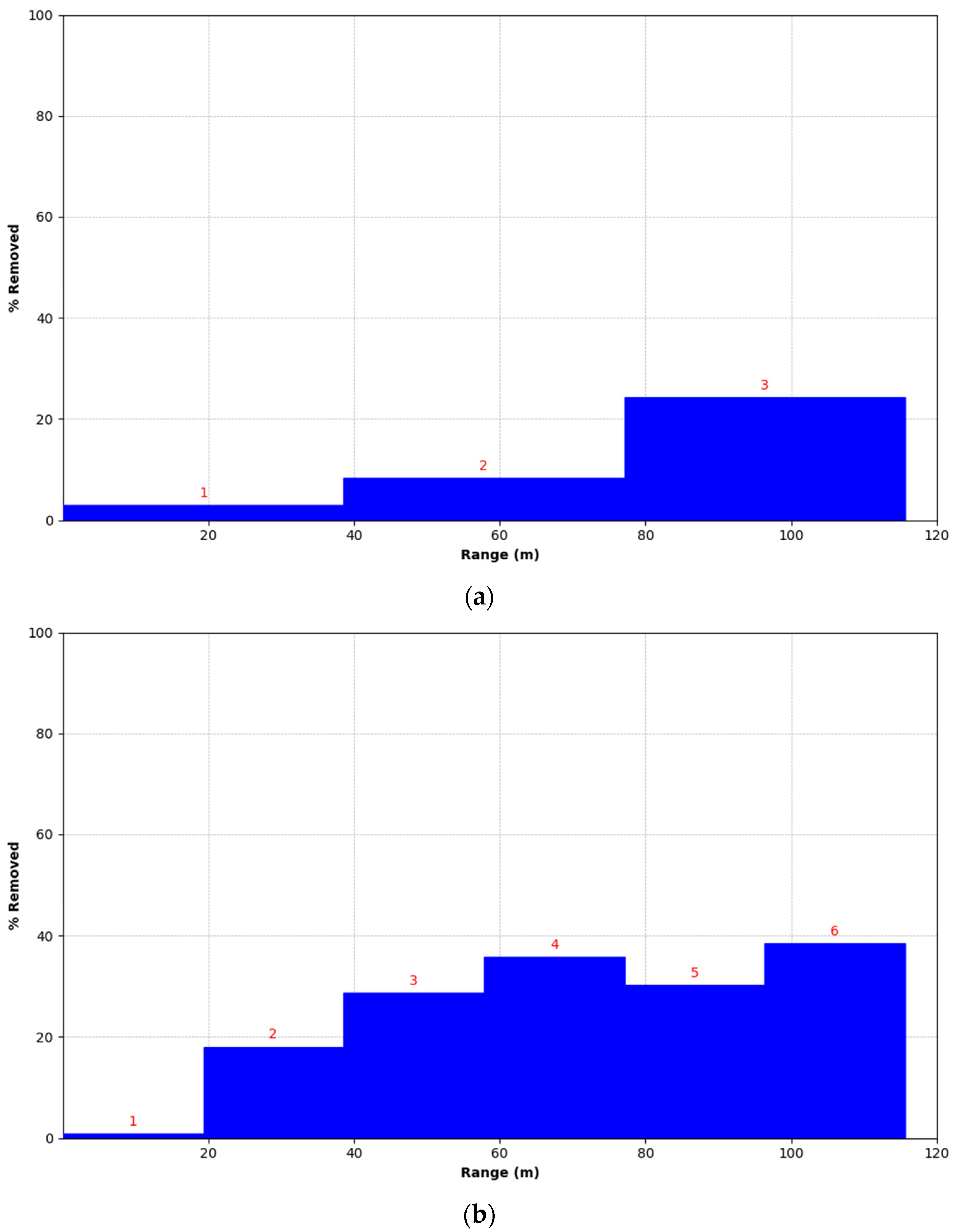
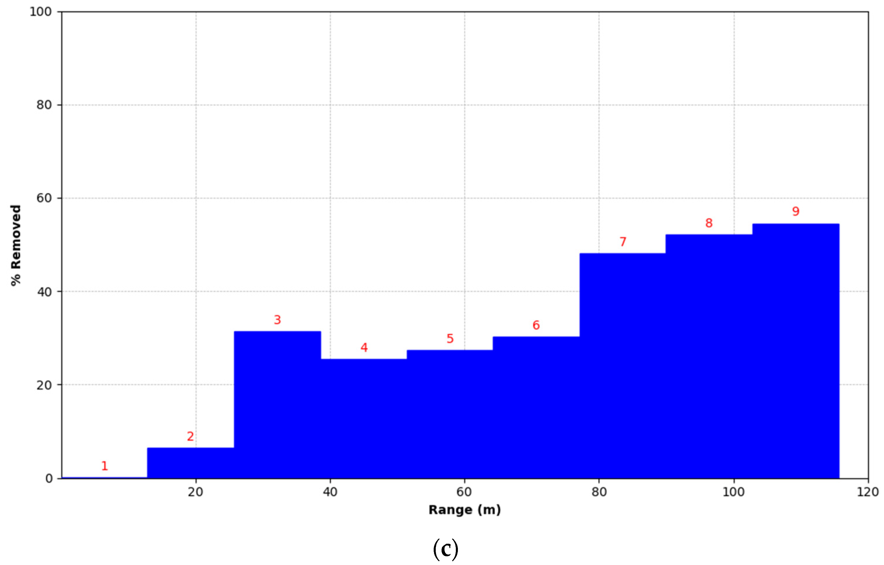
Spatial distribution of data points in different ranges

To thoroughly analyze the spatial distribution characteristics of the raw point cloud, a histogram was constructed (see Figure 3), which displays the distribution of point distances relative to the center of the LiDAR system. In this histogram, the horizontal axis is divided into intervals of 10 m, representing the distances from the data points to the center of the LiDAR; the vertical axis indicates the number of data points within each distance interval.

The histogram clearly illustrates a significant phenomenon: as distance increases, the density of point clouds decreases, a trend consistent with the intrinsic measurement characteristics of LiDAR (see Figure 4). Specifically, within a 10 m radius near the center of the LiDAR, the point cloud density is at its highest, reflecting its high resolution and excellent detection capabilities for nearby targets. As the distance extends, the density of point clouds gradually diminishes, primarily due to the sparse distribution of objects within the scanned area. At greater distances, the density significantly reduces due to a combination of factors including the device’s maximum effective detection range, laser beam divergence, atmospheric scattering, and the low reflectivity of target surfaces. The histogram provides an intuitive understanding of the LiDAR’s detection capabilities and the characteristics of its scanning area, which is crucial for the subsequent processing and analysis of point cloud data in outdoor real-world scenes.

(2)

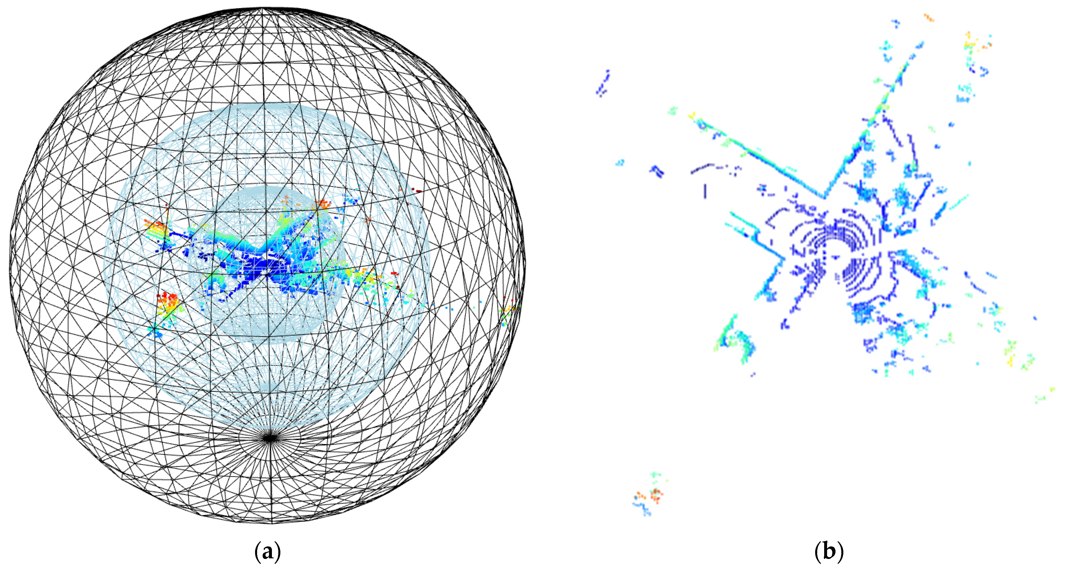
Denoising of point cloud data under equidistant segmentation in spherical space

Point cloud data collected in outdoor real-world scenes often exhibit sparsity and non-uniform distributions. When conventional denoising techniques are applied to such data, multiple parameter adjustments are typically required, and the results often fail to meet ideal denoising criteria. To address this issue, this study introduces a hierarchical denoising method based on equidistant segmentation within spherical space, which has been tested using point cloud data gathered from outdoor scenes. According to Formula (2), this study sets three different quantities of point cloud subsets: 3, 6, and 9. The denoising performance for each is illustrated in Figure 5, Figure 6 and Figure 7, respectively.

Figure 5, Figure 6 and Figure 7 illustrate the hierarchical denoising of point clouds under the equidistant segmentation in spherical space. The average performance of points removed from each point cloud subset under the equidistant segmentation is shown in Figure 8a–c, respectively.

An analysis of Figure 8a–c reveals that the denoising ratio varies significantly across different ranges as the number of point cloud subsets increases. Specifically, within approximately 13 m of the LiDAR center, the denoising ratio shows a gradual decline. Conversely, at distances greater than about 77 m from the LiDAR center, especially when the number of point cloud subsets is 9, the denoising ratio significantly increases. This phenomenon is attributed to the sparsity and extremely low density of point clouds in these ranges, as confirmed by the statistical distribution of point cloud quantities shown in Figure 3 and the trend of point cloud density with distance illustrated in Figure 4. Further comparative analysis from Figure 5b to Figure 7b indicates that with an increase in the number of subsets, the noise removal becomes more precise, particularly in areas far from the radar center. This improvement is due to the denoising algorithm which operates based on the proximity and number of points, thereby enhancing the overall denoising effect. Experimental results suggest that appropriately increasing the number of subsets can effectively optimize the performance of the denoising algorithm.

(3)

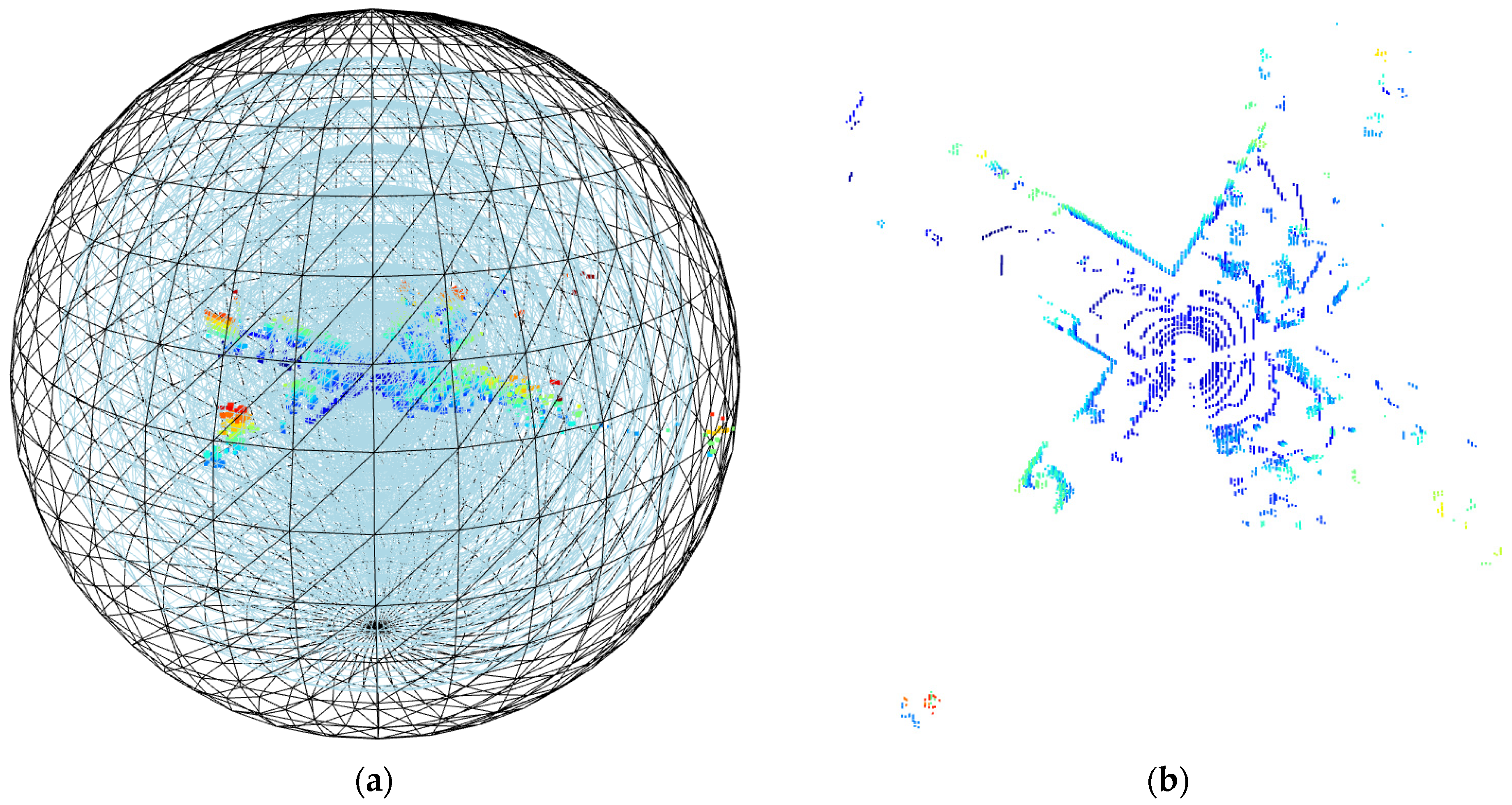
Denoising of point cloud data under proportional segmentation in spherical space

Raw data acquired from LiDAR typically exhibit spatial variations in point cloud density: regions near the center of the scanner have higher densities, resulting in more densely packed point clouds, whereas areas further from the center are less dense and thus sparser. Given that the proposed denoising method performs better on uniformly dense point clouds, a hierarchical denoising algorithm based on proportional segmentation in spherical space has been further developed. According to Formula (2), similar to the equidistant segmentation, the number of point cloud subsets was set at 3, 6, and 9 for the denoising experiments, with the results displayed in Figure 9, Figure 10 and Figure 11, respectively.

Figure 8, Figure 9 and Figure 10 illustrate the hierarchical denoising of point clouds under the proportional segmentation in spherical space. The average performance of points removed from each point cloud subset under the proportional segmentation is shown in Figure 12a–c, respectively.

An analysis of Figure 12a–c reveals that under proportional segmentation conditions, ranges closer to the center of the LiDAR generate a larger number of point cloud subsets. The substantial number of points in the range, coupled with an increased number of subsets, facilitates more precise control over noise removal. Particularly, when the subset count reaches 9, 6 subsets are formed within a 40 m radius of the LiDAR center. Compared to when there are only 3 or 6 subsets, the noise removal ratio in this region significantly improves, achieving more meticulous noise reduction. Beyond a 40 m radius from the LiDAR center, the noise removal ratio for 6 or 9 subsets significantly exceeds that for only 3 subsets. This phenomenon is mainly due to the sparse distribution and lower density of point clouds in that range. Further, analysis from Figure 9b to Figure 11b indicates that with 9 subsets, regardless of the proximity to the LiDAR center, the overall denoising effect of the point clouds is optimal.

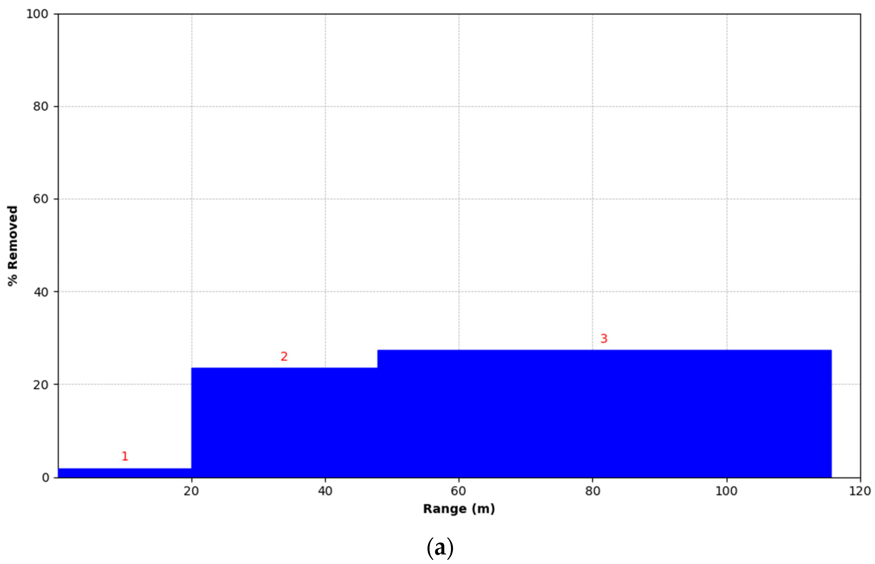
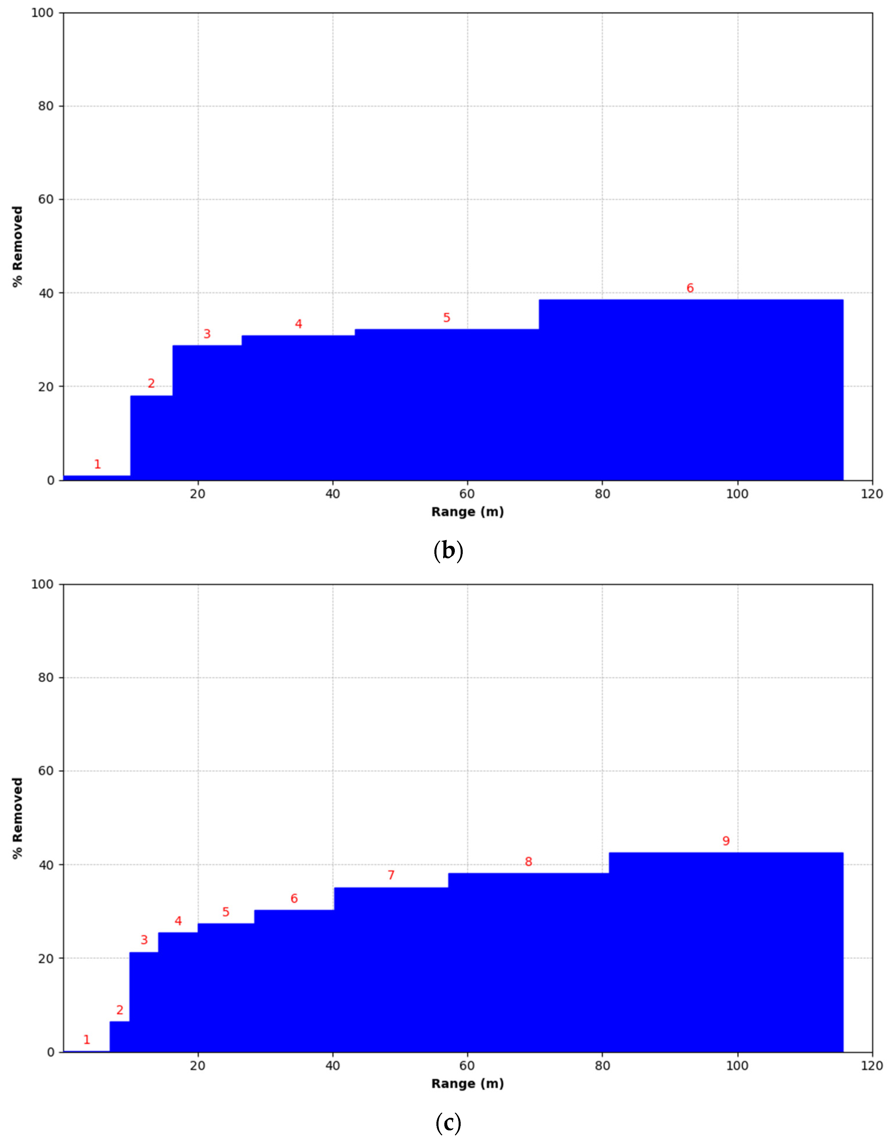
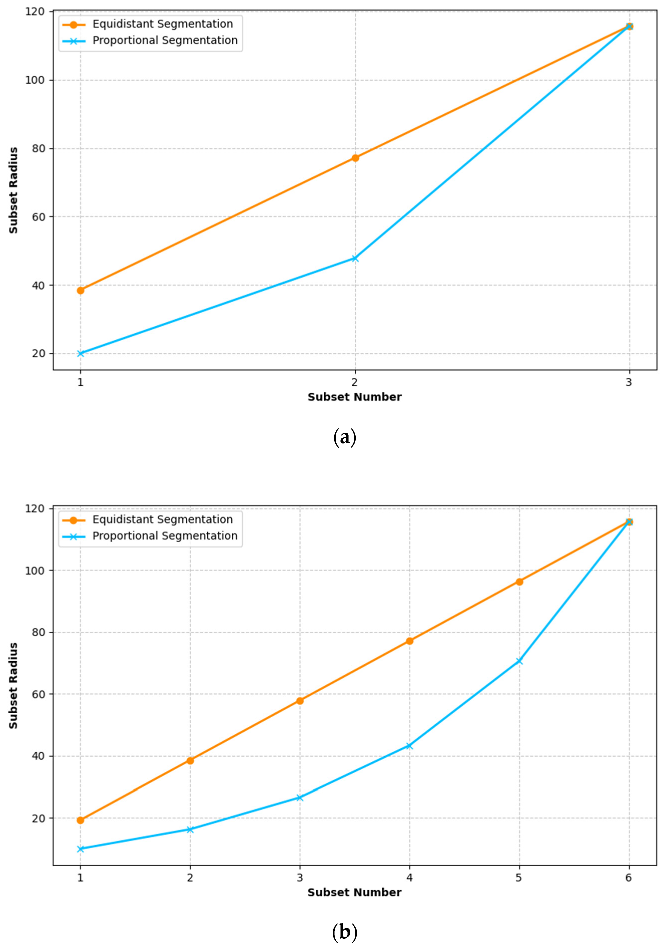
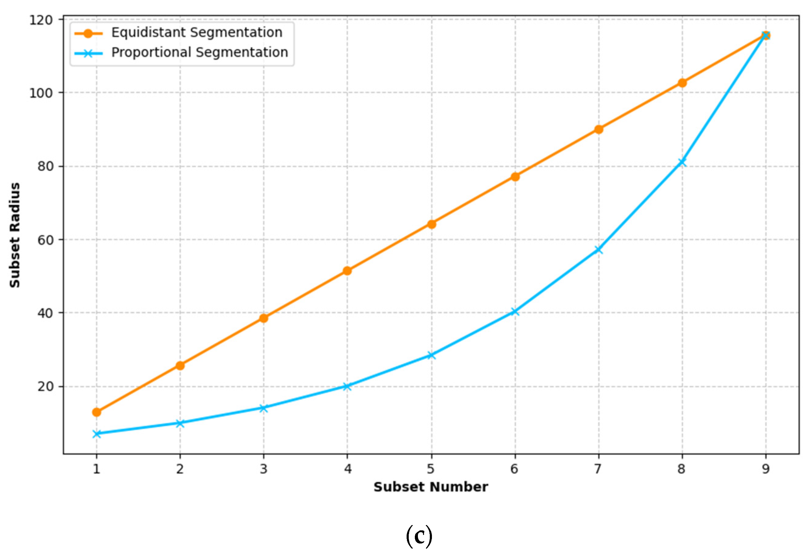
3.2.2. Quantitative Evaluation of Point Cloud Distribution under Equidistant and Proportional Segmentations

(1)

The radius of point cloud subsets under equidistant and proportional segmentations

To enhance the clarity and intuition of the variations in the radii of point cloud subsets under equidistant and proportional segmentations, this study illustrates the changes in radii for point clouds consisting of 3, 6, and 9 subsets under these segmentation conditions. The corresponding graphical results are displayed in Figure 13a–c, respectively.

As illustrated in Figure 13a, within a 40 m range of the LiDAR, both segmentation methods produce an equal number of subsets. Figure 13b,c shows that within the same distance, equidistant segmentation results in fewer subsets, while proportional segmentation yields more subsets, offering a finer segmentation. Approximately 94% of the point clouds are located within this range, yet with equidistant segmentation at 9 subsets, only 3 are generated. In areas with a vast number of points, fewer partitions mean that denoising parameters may lack specificity, adversely affecting the denoising outcome. In regions further from the center of the LiDAR (beyond 40 m), equidistant segmentation generates more subsets. Since the denoising algorithm analyzes based on the proximity and number of points, the sparsity of points in these regions might lead to inadvertent data deletion.

(2)

The overall standard deviation of point clouds after denoising

Standard deviation is commonly used to describe the variability of a dataset. In this study, the total standard deviation is utilized to evaluate the effectiveness of hierarchical segmentation of point clouds in spherical spaces through equidistant and proportional segmentations. Specifically, a lower total standard deviation indicates higher uniformity in the distribution of point clouds across different levels; conversely, a higher total standard deviation suggests significant disparities in uniformity among the levels. The uniformity of this distribution is quantified by the segmentation results of point clouds in spherical spaces, with the total standard deviation calculations presented in

Table 1. Total standard deviation under equidistant and proportional segmentations of spherical space.

Number of Subsets	Segmentation Strategy	TSD
3	ES	1.266
	PS	0.947
6	ES	1.177
	PS	0.683
9	ES	0.983
	PS	0.416

.

The analysis of Table 1 reveals that under the condition of an equal number of point cloud subsets, the total standard deviation for the proportional segmentation method is significantly lower than that for the equidistant segmentation method. This finding indicates that proportional segmentation in spherical spaces results in a more uniform distribution of point clouds across different hierarchies. Consequently, proportional segmentation not only optimizes the hierarchical division of point clouds in spherical spaces but also enhances the effectiveness of hierarchical denoising. These results highlight the importance of selecting an appropriate segmentation strategy when processing point cloud data.

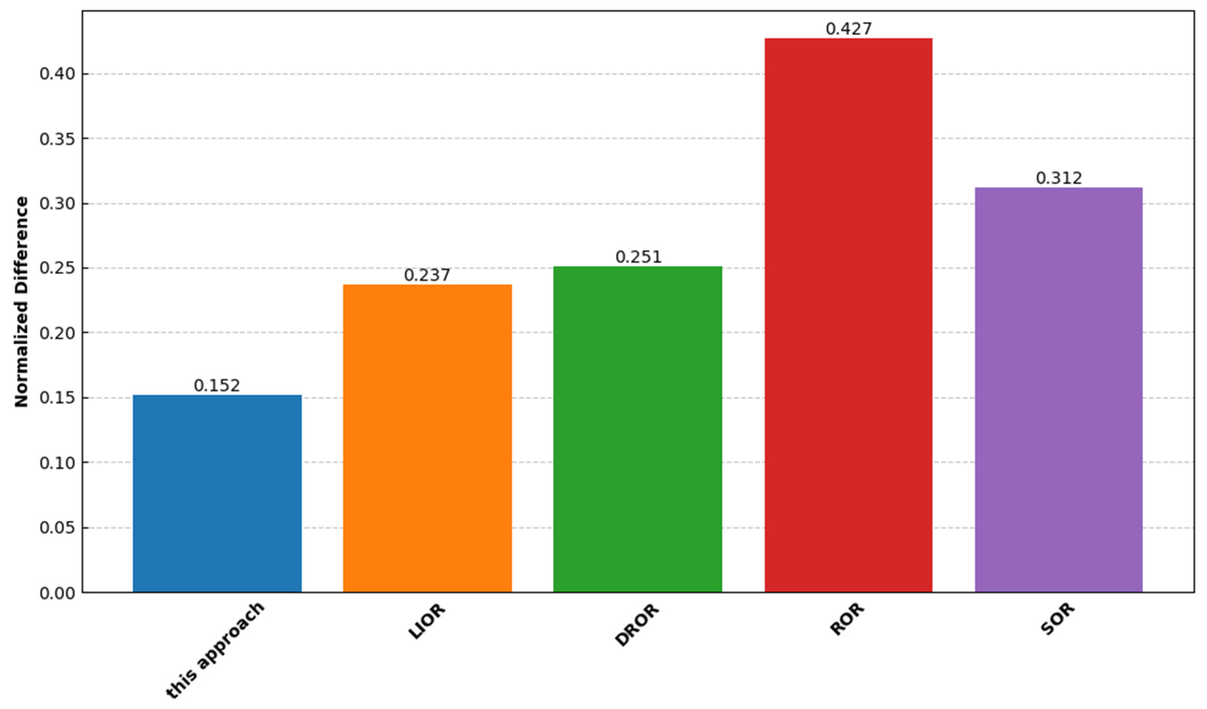
3.2.3. Point Cloud Denoising Effectiveness Assessment

(1)

The denoising performance of different denoising methods in outdoor real-world scenes

In outdoor real-world scenes, point cloud denoising operations should be conducted while preserving scene details and features of distant objects. Typically, the point cloud data acquired in outdoor real-world scenes exhibit significant variations in density. The point spacing between data points near the center of the LiDAR and those far from the center can differ by several tens to hundreds of times. Conventional point cloud denoising methods use fixed parameters for denoising, which cannot dynamically adjust based on changes in point cloud density. As a result, the denoising performance of these methods is highly sensitive to point cloud density and point spacing, making them suboptimal for denoising in outdoor real-world scenes. This study proposes a method that segments the point cloud into spatially hierarchical subsets, grouping point clouds with similar densities into the same subset. Each point cloud subset is then assigned denoising parameters appropriate for its density, thereby achieving more effective noise removal without losing scene details. To further evaluate the performance of the proposed method in removing noise from point clouds in outdoor real-world scenes, comparisons were made with ROR [22], SOR [22], DROR [21], and LIOR [23]. The results are presented in Figure 14.

In Figure 14a–g, (1) represents the car’s outer contour and the ground. Upon observation, it can be noted that there are some noise points at the edges of the car’s contour and on the ground. After applying the denoising method proposed in this study, the noise points around the car’s contour and on the ground were significantly reduced, as shown in Figure 14f,g-(1). The DROR and LIOR methods performed poorly, leaving a small amount of noise points after implementation. The ROR and SOR methods showed the worst performance, with noise points remaining quite evident after application. In Figure 14a–g, (2) represents the side façade of a building. Similarly, careful observation reveals that after the proposed adaptive parameter denoising under proportional measurable segmentation, the distant building retains a relatively complete geometric feature structure while being denoised, as shown in Figure 14g-(2). Other methods performed poorly, especially when an equidistant measurable segmentation method was applied to the point cloud set. The geometric structural features of distant objects were not well preserved during denoising. In Figure 14a–g, (3) represents the ground cover of junipers, with many noise points present within and around them. After applying the denoising method proposed in this study, the noise points in the point cloud were significantly reduced, especially when the proportional measurable segmentation method was adopted, as shown in Figure 14g-(3). The ROR, SOR, DROR, and LIOR methods showed average performance, with some noise points remaining unremoved in the point cloud after implementation. From the above analysis, it can be concluded that when the point cloud set undergoes adaptive parameter denoising based on proportional measurable segmentation, noise can be maximally removed while preserving the geometric structural features of objects, regardless of their proximity to or distance from the LiDAR center.

(2)

Comparing the efficiency of point cloud denoising methods

Given the typically large volume of point cloud data collected by LiDAR in outdoor environments, time efficiency becomes critically important during the denoising process. Therefore, this study has conducted a statistical analysis of the time required by various denoising methods under the same computational conditions (as described in Section 3.1.2), with specific results presented in

Table 2. Time statistics for different denoising methods.

	ROR	SOR	DROR	LIOR	This Approach
Denoising time (s)	8.154	0.503	7.731	3.287	2.793

.

An analysis of Table 2 reveals that among the methods for denoising point cloud data from outdoor scenes, the SOR method requires the least time, while the ROR method takes the most. The DROR method consumes slightly less time than ROR but is still more time-consuming than the LIOR. The denoising time with the studied method is greater than that of SOR but superior to the other three methods. Compared to the DROR method, this approach shows a time reduction of over 60%, and about 15% compared to the LIOR method. This layered adaptive parameter denoising method, based on measurable segmentation, processes the point cloud by dividing it into smaller sections, reducing the data volume per section and thereby diminishing the computational load per process. This distributed computational load implies that each section can be processed faster, especially when utilizing multicore or parallel processing. Moreover, by delineating the extent of each layer, the method allows the algorithm to dynamically adjust the denoising parameters according to the characteristics of each layer’s data, thereby more finely addressing the varying characteristics of different regions, such as point density and noise levels, reducing redundant computations of neighbor points, and ultimately decreasing the overall processing time.

(3)

Quantitative evaluation of different denoising methods

In the evaluation of noise removal efficacy within real-world outdoor scenes, acquiring high-quality real point cloud datasets often presents a challenge. To ensure a fair comparison between the denoising method proposed in this study and other approaches, such as LIOR, DROR, SOR, and ROR, this study has adopted the normalized median variance as the metric to quantify the performance of different denoising techniques. This approach is based on each point in the denoised point cloud, where it seeks neighboring points in the raw dataset and calculates the variance of these points. This variance measures the consistency and stability of point distributions within local areas. The median, rather than the mean, of these variances is used as the metric to effectively reduce the impact of outliers on the evaluation results. Subsequently, this median variance is normalized to ensure consistency and fairness in the evaluation results across different scales of data. Figure 15 illustrates a comparison of the denoising performance achieved by five different filters.

Figure 15 presents a quantitative comparison of the performance of five denoising filters, assessed using the normalized median variance difference. A smaller normalized value indicates that the denoised point cloud retains a higher degree of local spatial consistency with the raw point cloud. The results suggest that the denoising method proposed in this study exhibits the smallest normalized difference, indicating superior denoising performance in real-world outdoor scenes. In comparison, the LIOR, DROR, and SOR filters perform moderately well, while the ROR filter shows the least desirable denoising outcomes.

4. Discussion

4.1. Efficacy of Point Cloud Hierarchical Denoising with Spherical Space Measurable Segmentation

The hierarchical denoising method for point clouds, through measurable segmentation of spherical space, has demonstrated its efficacy in point cloud data processing. This approach employs a step-by-step denoising strategy, dynamically adjusting the denoising parameters to align with the distance between data points and the LiDAR center, making it particularly suitable for noisy, sparse, and non-uniform point cloud data while effectively preserving the detailed features of the point clouds. Moreover, it offers a range of adjustable parameters, such as the horizontal and vertical resolutions of LiDAR and the number of concentric spheres, allowing users to customize the method based on the specific characteristics of the data, thereby enhancing its applicability. Most critically, the method supports the visualization of concentric spheres and point clouds both before and after denoising, providing researchers and users with a powerful tool to visually assess the denoising outcomes.

4.2. Limitations of Point Cloud Hierarchical Denoising with Spherical Space Measurable Segmentation

While the denoising method proposed in this study demonstrates certain advantages, it also possesses inherent limitations. Firstly, when processing large-scale point cloud datasets, the sequential handling of multiple concentric spheres increases computation time, which may render this method unsuitable for applications requiring real-time processing. Secondly, the performance of this method depends on the assumption that the point cloud data are concentrically distributed. Deviations from this assumption could adversely affect performance. Therefore, in practical applications, a precise understanding of the distribution characteristics of point cloud data in outdoor scenes is especially critical.

4.3. The Practicality Extension and Computational Efficiency Optimization of the Hierarchical Denoising Method

The point cloud denoising method proposed in this study demonstrates certain advantages over traditional techniques [17], particularly in preserving fine details, especially when dealing with unevenly distributed noise, offering new perspectives and solutions for point cloud processing. To enhance the efficiency and applicability of this method, it is essential to explore and implement computational optimization strategies, especially to reduce the computational time required for processing large point cloud datasets [24]. Additionally, the introduction of an automatic parameter adjustment mechanism allows for the automation of the denoising parameter selection, optimized according to the characteristics of the point cloud distribution, further enhancing the practicality of the method.

5. Conclusions

This study presents a method for the hierarchical denoising of a point cloud within a finite measurable segmentation framework in spherical space, and its efficacy is empirically demonstrated. By gradually increasing the radii of concentric spheres and finely tuning the parameters, the method successfully eliminated noise and outliers in the point cloud. The denoised data closely resembled the geometric shapes of the original scene, significantly enhancing the quality and usability of the data. However, this study also highlights the importance of parameter selection, urging researchers to choose appropriate parameters based on their specific datasets and application scenes to achieve optimal denoising results. Future work may include more sophisticated methods for adaptive parameterization and performance optimization in various applications. Overall, the hierarchical denoising method under finite measurable segmentation in spherical space provides an effective solution for point cloud denoising, with potential for further research and innovative improvements for practical applications.

References

- Yang, B.; Haala, N.; Dong, Z. Progress and Perspectives of Point Cloud Intelligence. Geo-Spat. Inf. Sci. 2023, 26, 189–205. [Google Scholar] [CrossRef]
- Wirth, F.; Quchl, J.; Ota, J.; Stiller, C. PointAtMe: Efficient 3D Point Cloud Labeling in Virtual Reality. In Proceedings of the 2019 30th IEEE Intelligent Vehicles Symposium (IV), Paris, France, 9–12 June 2019; pp. 1693–1698. [Google Scholar]
- Valenzuela-Urrutia, D.; Muñoz-Riffo, R.; Ruiz-del-Solar, J. Virtual Reality-Based Time-Delayed Haptic Teleoperation Using Point Cloud Data. J. Intell. Robot. Syst. 2019, 96, 387–400. [Google Scholar] [CrossRef]
- Tredinnick, R.; Broecker, M.; Ponto, K. Progressive Feedback Point Cloud Rendering for Virtual Reality Display. In Proceedings of the 2016 IEEE Virtual Reality Conference (VR), Greenville, SC, USA, 19–23 March 2016; pp. 301–302. [Google Scholar]
- Alexiou, E.; Upenik, E.; Ebrahimi, T. Towards Subjective Quality Assessment of Point Cloud Imaging in Augmented Reality. In Proceedings of the 2017 19th IEEE International Workshop on Multimedia Signal Processing (MMSP), Luton, UK, 16–18 October 2017. [Google Scholar]
- Ma, K.; Lu, F.; Chen, X.W. Robust Planar Surface Extraction from Noisy and Semi-dense 3D Point Cloud for Augmented Reality. In Proceedings of the 2016 International Conference on Virtual Reality and Visualization (ICVRV), Hangzhou, China, 24–26 September 2016; pp. 453–458. [Google Scholar]
- Lin, X.H.; Wang, F.H.; Yang, B.S.; Zhang, W.W. Autonomous Vehicle Localization with Prior Visual Point Cloud Map Constraints in GNSS-Challenged Environments. Remote Sens. 2021, 13, 506. [Google Scholar] [CrossRef]
- Chen, S.H.; Liu, B.A.; Feng, C.; Vallespi-Gonzalez, C.; Wellington, C. 3D Point Cloud Processing and Learning for Autonomous Driving: Impacting Map Creation, Localization, and Perception. IEEE Signal Process. Mag. 2021, 38, 68–86. [Google Scholar] [CrossRef]
- Xiao, Z.P.; Dai, B.; Li, H.D.; Wu, T.; Xu, X.; Zeng, Y.J.; Chen, T.T. Gaussian Process Regression-Based Robust Free Space Detection for Autonomous Vehicle by 3-D Point Cloud and 2-D Appearance Information Fusion. Int. J. Adv. Robot. Syst. 2017, 14, 172988141771705. [Google Scholar] [CrossRef]
- Abellan, A.; Derron, M.-H.; Jaboyedoff, M. “Use of 3D Point Clouds in Geohazards” Special Issue: Current Challenges and Future Trends. Remote Sens. 2016, 8, 130. [Google Scholar] [CrossRef]
- Cai, X.H.; Lü, Q.; Zheng, J.; Liao, K.W.; Liu, J. An Efficient Adaptive Approach to Automatically Identify Rock Discontinuity Parameters Using 3D Point Cloud Model from Outcrops. Geol. J. 2023, 58, 2195–2210. [Google Scholar] [CrossRef]
- Jung, M.Y.; Jung, J.H. A Scalable Method to Improve Large-Scale Lidar Topographic Differencing Results. Remote Sens. 2023, 15, 4289. [Google Scholar] [CrossRef]
- Mammoliti, E.; Di Stefano, F.; Fronzi, D.; Mancini, A.; Malinverni, E.S.; Tazioli, A. A Machine Learning Approach to Extract Rock Mass Discontinuity Orientation and Spacing, from Laser Scanner Point Clouds. Remote Sens. 2022, 14, 2365. [Google Scholar] [CrossRef]
- Javaheri, A.; Brites, C.; Pereira, F.; Ascenso, J. Subjective and Objective Quality Evaluation of 3D Point Cloud Denoising Algorithms. In Proceedings of the 2017 IEEE International Conference on Multimedia & Expo Workshops (ICMEW), Hong Kong, China, 10–14 July 2017; pp. 1–6. [Google Scholar]
- Mian, A.; Bennamoun, M.; Owens, R. On the Repeatability and Quality of Keypoints for Local Feature-Based 3D Object Retrieval from Cluttered Scenes. Int. J. Comput. Vis. 2010, 89, 348–361. [Google Scholar] [CrossRef]
- Digne, J. Similarity Based Filtering of Point Clouds. In Proceedings of the 2012 IEEE Computer Society Conference on Computer Vision and Pattern Recognition Workshops, Providence, RI, USA, 16–21 June 2012; pp. 73–79. [Google Scholar]
- Cheng, D.; Zhao, D.; Zhang, J.; Wei, C.; Tian, D. PCA-Based Denoising Algorithm for Outdoor Lidar Point Cloud Data. Sensors 2021, 21, 3703. [Google Scholar] [CrossRef] [PubMed]
- Sun, G.; Chu, C.; Mei, J.; Li, W.; Su, Z. Structure-Aware Denoising for Real-world Noisy Point Clouds with Complex Structures. Comput.-Aided Des. 2022, 149, 103275. [Google Scholar] [CrossRef]
- Zheng, Z.; Zha, B.; Zhou, Y.; Huang, J.; Xuchen, Y.; Zhang, H. Single-Stage Adaptive Multi-Scale Point Cloud Noise Filtering Algorithm Based on Feature Information. Remote Sens. 2022, 14, 367. [Google Scholar] [CrossRef]
- Shi, C.; Wang, C.; Liu, X.; Sun, S.; Xiao, B.; Li, X.; Li, G. Three-Dimensional Point Cloud Denoising via a Gravitational Feature Function. Appl. Opt. 2022, 61, 1331–1343. [Google Scholar] [CrossRef]
- Charron, N.; Phillips, S.; Waslander, S.L. De-noising of Lidar Point Clouds Corrupted by Snowfall. In Proceedings of the 2018 15th Conference on Computer and Robot Vision (CRV), Toronto, ON, Canada, 8–10 May 2018; pp. 254–261. [Google Scholar]
- Rusu, R.B.; Cousins, S. 3D is here: Point Cloud Library (PCL). In Proceedings of the 2011 IEEE International Conference on Robotics and Automation, Shanghai, China, 9–13 May 2011; pp. 1–4. [Google Scholar]
- Park, J.-I.; Park, J.; Kim, K.-S. Fast and Accurate Desnowing Algorithm for LiDAR Point Clouds. IEEE Access 2020, 8, 160202–160212. [Google Scholar] [CrossRef]
- Elseberg, J.; Borrmann, D.; Nüchter, A. Efficient Processing of Large 3D Point Clouds. In Proceedings of the 2011 XXIII International Symposium on Information, Communication and Automation Technologies, Sarajevo, Bosnia and Herzegovina, 27–29 October 2011; pp. 1–7. [Google Scholar]