Abstract
Floods are among the most common disasters, causing loss of life and enormous damage to private property and public infrastructure. Monitoring systems that detect and predict floods help respond quickly in the pre-disaster phase to prevent and mitigate flood risk and damages. Thus, this paper presents a deep neural network (DNN)-based real-time flood monitoring system for embedded Internet of Things (IoT) edge devices. The proposed system fuses long-wave infrared (LWIR) and RGB cameras to overcome a critical drawback of conventional RGB camera-based systems: severe performance deterioration at night. This system recognizes areas occupied by water using a DNN-based semantic segmentation network, whose input is a combination of RGB and LWIR images. Flood warning levels are predicted based on the water occupancy ratio calculated by the water segmentation result. The warning information is delivered to authorized personnel via a mobile message service. For real-time edge computing, the heavy semantic segmentation network is simplified by removing unimportant channels while maintaining performance by utilizing the network slimming technique. Experiments were conducted based on the dataset acquired from the sensor module with RGB and LWIR cameras installed in a flood-prone area. The results revealed that the proposed system successfully conducts water segmentation and correctly sends flood warning messages in both daytime and nighttime. Furthermore, all of the algorithms in this system were embedded on an embedded IoT edge device with a Qualcomm QCS610 System on Chip (SoC) and operated in real time.
1. Introduction
Natural disasters such as floods, forest fires, earthquakes, and landslides have steadily increased over the past few decades, and the frequency of their occurrence is also rapidly growing. These disasters cause heavy loss of human life and destruction of private property and public infrastructure and leave behind significant social and economic damages. The process of a disaster consists of three phases: pre-disaster (before the disaster), intra-disaster (during the disaster), and post-disaster (after the disaster) [1,2]. The ultimate goal of disaster management (DM) is to prevent and mitigate the loss of life and disaster risk. The most effective way to do this is to detect disasters early and respond quickly and promptly. This is why a DM system in the pre-disaster phase, consisting of prediction, monitoring, and early warning, is indispensable.
Flooding is one of the most common disasters, accounting for 44% of all disasters from 2000 to 2019 [3]. In the pre-disaster phase, the monitoring system can detect flooding early, and the emergency warning system can help evacuate people in hazardous areas quickly to prevent massive damage. The traditional approach to predicting flooding, a type of hydrological event, typically utilizes hydrological and meteorological data such as water levels, water discharge, rainfall, and wind direction, measured directly by various sensors [4,5]. However, the sensors used in this approach are limited to being installed in specific places and have a narrow detection range; they are unable to recognize the progress of floods in various locations, and the measured data cannot be visualized, making it difficult to understand the actual site.
On the other hand, image sensors have a more comprehensive detection range than conventional direct measurement sensors and can provide more information about the river and its surroundings. In recent years, advances in deep learning (DL) technology have improved the accuracy of image processing techniques in computer vision, which has led to more research on detecting water bodies in rivers based on images to predict floods. Depending on the image acquisition technology, imagery data for flood detection are categorized into satellite imagery, unmanned aerial vehicle (UAV) imagery, and surveillance camera imagery. Satellite imagery covers a large area, making it difficult to extract specific information from a small area, and the long observation interval of satellites makes them unsuitable for real-time flood monitoring. UAVs have been utilized as a suitable technology for flood monitoring due to their ability to acquire high-resolution images at low altitudes [6,7,8]. However, due to their small size, the performance of data accuracy in terms of resolution can be affected during severe weather conditions such as heavy rain or typhoons. In addition, it is difficult for a UAV to monitor for an extended duration because it has to handle various tasks such as flight and image acquisition and processing with limited resources. In the end, surveillance cameras that can reliably acquire and process data over a small area are an effective alternative for flood monitoring. Utilizing surveillance cameras for flood monitoring has the benefit of reducing costs for new camera installation because it is possible to use existing surveillance cameras in some cases. In addition, newly installed flood monitoring cameras can be utilized for other purposes, such as vehicle and pedestrian surveillance.
There are three challenges in realizing an image-based flood monitoring system using a deep neural network (DNN): (1) It is necessary to detect changes in rivers and streams regardless of whether it is day or night. (2) Edge-computing-based flood detection is required for real-time responses to floods, which means image analysis on camera devices that acquire images. (3) A warning system is needed to notify people in the hazardous area of an emergency so that they can evacuate quickly.
This paper proposes a DNN-based flood monitoring system fusing RGB and long-wave infrared (LWIR) cameras for embedded Internet of Things (IoT) edge devices. First, we propose using an LWIR sensor to identify changes in river water bodies, even at night. Using only an RGB sensor makes it very difficult to distinguish objects in the images at night due to insufficient illumination. Furthermore, RGB images are affected by poor weather conditions, such as fog or heavy rain, so fusion with other sensors is necessary [9]. Unlike RGB sensors, LWIR sensors output images in response to infrared heat emitted from objects. Thus, even in the case of weather changes or during the night, our system can obtain stable image data from the LWIR sensor without much difference from daytime in clear weather. We also use a network slimming method for AI edge computing. This method has the effect of significantly reducing the size and computation of the heavy network with the same accuracy. Next, we deploy the lightweight network to the edge devices and obtain the inference results. Finally, we verify that the implemented warning message generation module sends flood warning messages successfully.
The contributions of this paper are as follows:
- (1)
- To the best of our knowledge, this is a novel system to monitor floods using a multimodal camera sensor composed of RGB and LWIR. This multimodal sensor-based approach improved the performance of water segmentation for night images.
- (2)
- For edge computing, we applied a network slimming method to DeepLabV3+, a semantic segmentation network that segments water in RGB and LWIR fused images. The method resulted in a significant reduction in processing time without degrading performance.
- (3)
- To verify the practicality and effectiveness of the proposed method, we demonstrated it in embedded using Qualcomm’s SoC (System on Chip).
- (4)
- A flood warning system module based on a mobile message service was built and demonstrated.
2. Related Works
This paper focuses on flood monitoring based on surveillance cameras. This section summarizes related works on DNN-based flood monitoring and detection from surveillance cameras.
Early approaches focused on segmenting water regions in images by applying existing DNN-based segmentation algorithms. Lopez-Fuentes et al. [10] proposed a flood monitoring system that automatically analyzes images from surveillance cameras to predict floods. It was almost the first attempt to use a DNN-based segmentation algorithm to segment water regions in river images instead of conventional texture or color-based image processing algorithms. They compared the performance of three different segmentation algorithms in their experiments. The results showed that their work is suitable for implementing automatic detection of water level rises for flood early warning. Baydargil et al. [11] conducted a study to detect whether a road is flooded using surveillance cameras monitoring the road. They used SegNet to segment flooded regions on the road. Akiyama et al. [12] installed surveillance cameras around a river to acquire image data and used SegNet to perform water segmentation.
After these studies, there was research on predicting water levels from water segmentation results: approaches using flood index [13], approaches using classification algorithm [14], and approaches using landmarks [15,16].
Vitry et al. [13] proposed a novel approach to identify water level trends from existing surveillance camera systems. They used a DNN algorithm to detect floods in the image and proposed a new flood index to predict the water level. The flood index is calculated as the ratio of the water region to the region of interest in the image as an indicator of visible water level fluctuations. The experimental results showed that the predicted flood index highly correlated with the water level a conventional ultrasonic rangefinder measured.
Borwarninginn et al. [14] proposed a method for detecting water levels in surveillance cameras. They used an approach based on a classification algorithm that sets water levels into several classes and outputs them from the input image. They used InceptionV3 as a DNN-based classification algorithm. Also, they proposed a new model incorporating an attention mechanism so that a single model can be utilized for multiple surveillance cameras.
Vandaele et al. [15] proposed a method to predict flood risk based on water level obtained from water segmentation results for automatic flood detection. They used FCN, UperNet, and DeepLabv2 on surveillance camera images installed around a river for water segmentation. They marked landmarks in the images, which are indicators for predicting water level, and predicted water level and flood risk by determining whether the segmented water region contains landmarks. Muhadi et al. [16] proposed a flood detection method based on landmarks, similar to [15]. They used DeepLabv3+ and SegNet to detect water bodies in surveillance images. The experimental results showed that DeepLabv3+ outperformed SegNet. They used water level markers to estimate the water level from the detected water bodies, which were determined using LiDAR data information. These markers were also used as indicators of the flood warning level. The experimental results reported that the predicted water level was highly correlated with the water level directly measured by the water level sensor.
Other research has focused on how to simplify DNNs in flood detection applications to deploy deep learning models on edge devices. Fernandes et al. [17] proposed a pruning algorithm to lighten the DNNs used for water segmentation. Since deploying DNN models with large sizes in resource-constrained edge devices is a challenging problem, they researched a pruned model that fits into a specific memory without degrading performance. They used DeepLabv3 and proposed a randomized heuristic-based pruning algorithm. The experimental results showed that the proposed algorithm could find pruned models with adequate performance within the specified amount of memory. Our previous work [18] applied a semantic segmentation network to public forest fire and flood datasets for forest fire and flood detection. We simplified the network by utilizing a network slimming method and showed that the simplified semantic segmentation network operated in real time on an embedded board.
In summary, most of the existing studies have focused on segmenting water and predicting water levels from surveillance camera images for flood monitoring. And they have shown that DNN-based segmentation algorithms perform well enough to be used for flood detection and that this approach has sufficient potential to be used in flood monitoring systems. In addition, most of the experiments have been conducted on GPU-based desktop environments and image datasets acquired during the daytime. Few studies have shown the results of lightweight DNNs and ported them to real edge devices for real-time flood monitoring systems.
3. Flood Monitoring System
3.1. Overview
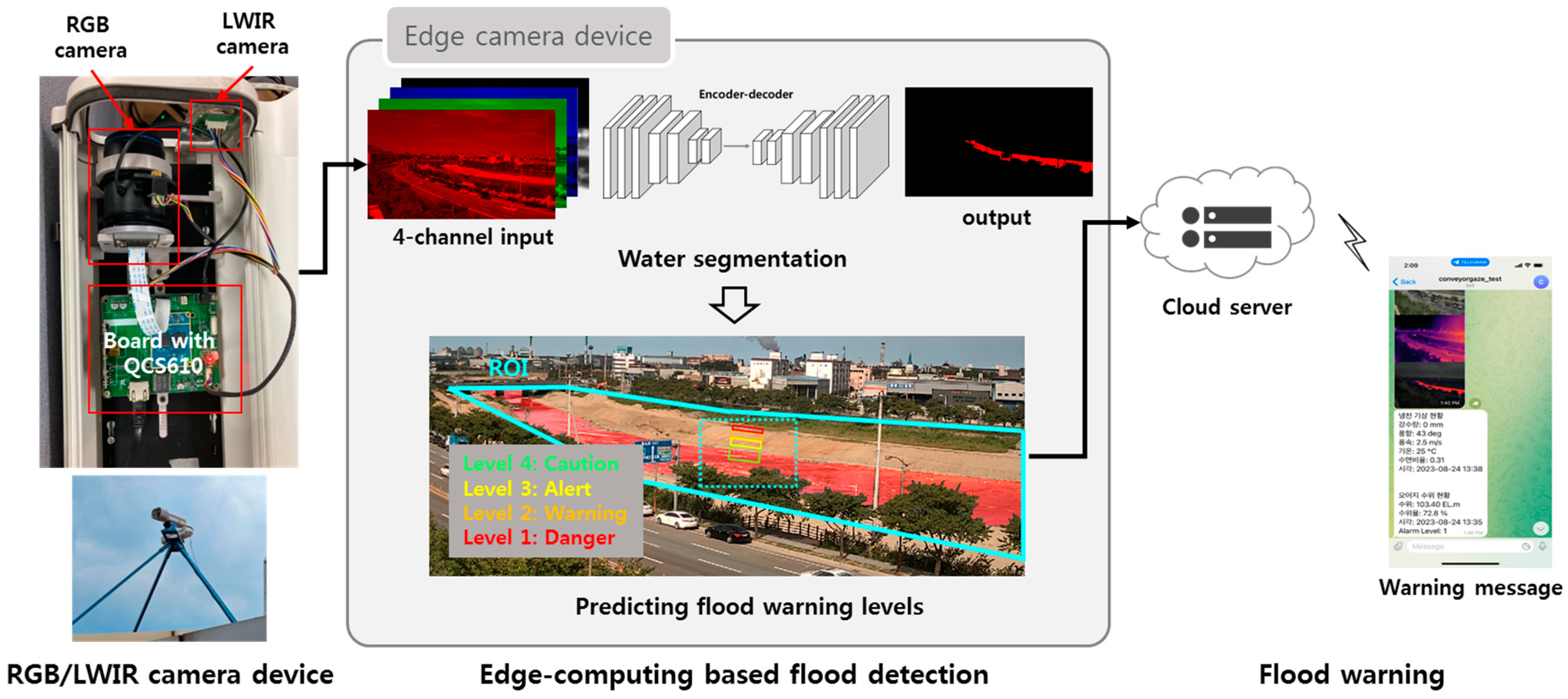
Figure 1 shows the overall process of the proposed flood monitoring system. The proposed system consists of three stages: image acquisition and preprocessing, edge-computing-based flood detection, and flood warning. In the first stage, RGB and LWIR images obtained from multimodal sensor-based surveillance cameras are matched. In the next stage, water segmentation results are obtained using a DNN-based semantic segmentation network on the SoC mounted on the camera board. In addition, the flood hazard area is set as the region of interest (ROI) in the image, and the predicted flood warning level is output by calculating the proportion of water regions in the ROI. In the last step, the flood warning level is sent to the cloud server, and the generated warning message based on this flood level is delivered to the authorized users’ cell phones or PCs.
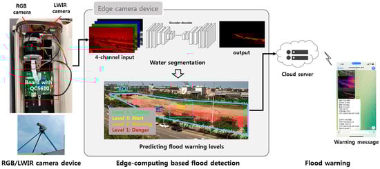
Figure 1.
Overview of the proposed flood monitoring system.
3.2. Alignment of RGB and LWIR Images
In the alignment stage, we combine RGB three-channel images with LWIR one-channel images and use four channels of fused data as input. However, since the RGB and LWIR camera lenses are located side by side in the camera device, each sensor acquires images from different viewpoints. To generate four channels of fused input data, the viewpoints of the RGB and LWIR images must be matched in a process called image alignment. To this end, we used a projective transformation (homography) for the relation between RGB and LWIR images. In the proposed system, the RGB and LWIR cameras are incredibly close to each other, and the target object is considerably far from them. Therefore, the relation between a pair of images captured by the two cameras can surely be approximated by homography [19]. We have measured the alignment accuracy by calculating the average distance between the corresponding points after the alignment. It was 5.02 pixels (0.87% with respect to the diagonal distance of the input image).
Image alignment starts by obtaining corresponding points between the RGB and LWIR images. Next, a homography matrix is computed using these correspondence points. Then, the homography matrix is applied to the LWIR image to transform the LWIR image to match the RGB image. Finally, four channels of fused data are generated by concatenating three channels of the RGB image and one channel of the LWIR image. Figure 2 shows the process of aligning RGB and LWIR images. In this process, the corresponding points do not need to be detected repeatedly for every input image. This is because the homography matrix determined once in the camera settings can be used continuously for newly acquired RGB and LWIR input images.
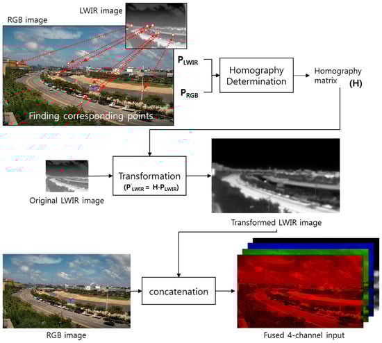
Figure 2.
Image alignment process using homography.
3.3. Semantic Segmentation: DeepLabv3+
The DeepLab series [20,21,22,23] was developed by Google Research and is known for its high performance among semantic segmentation networks. DeepLabv3+ [20] is the most recently updated model and has the best performance compared to previous versions of DeepLab models.
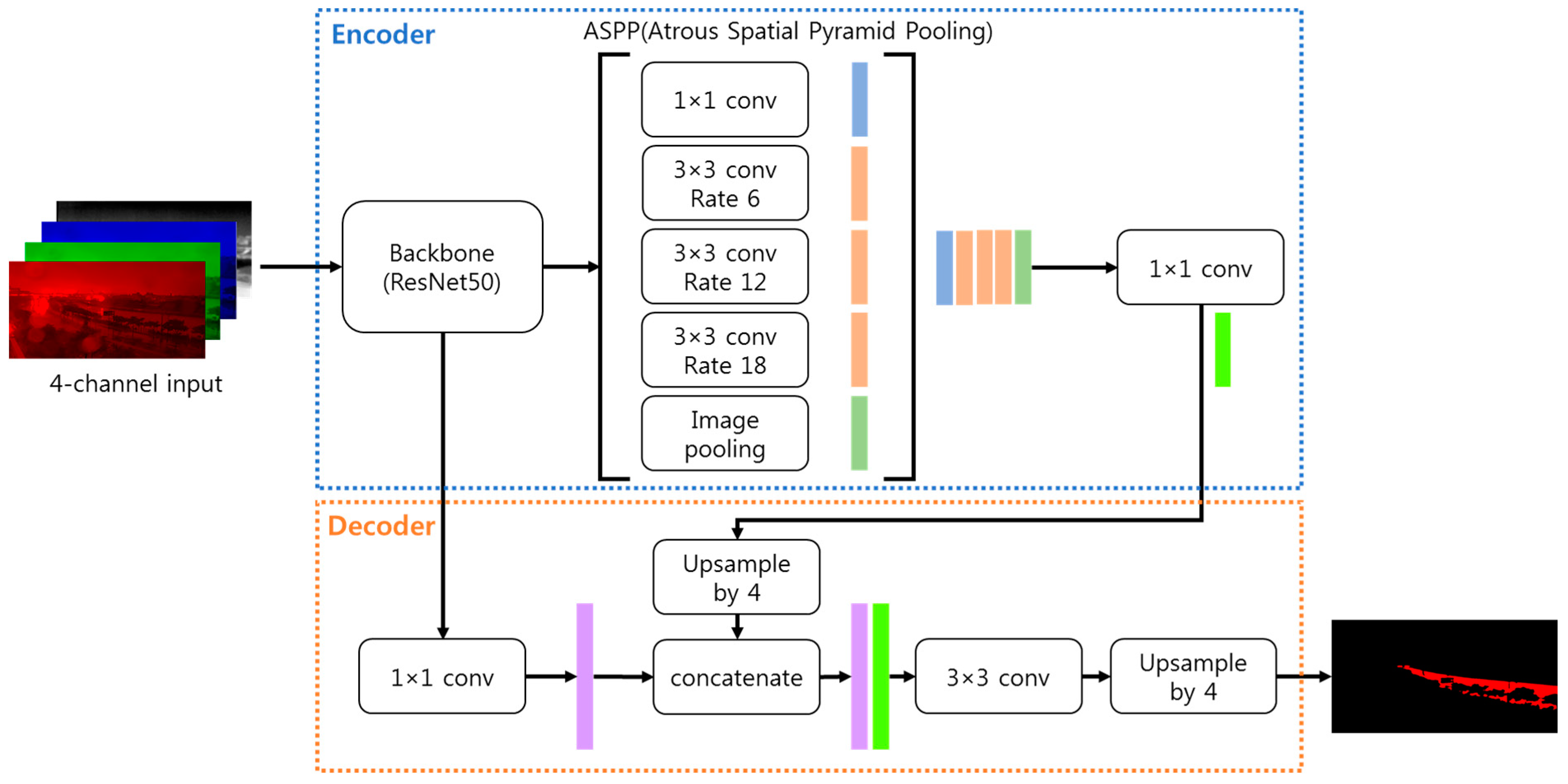
The main feature of DeepLabv3+ that differs from previous versions is the addition of a simple but effective decoder module. This decoder helps effectively recover the details of the segmented object boundary. As shown in Figure 3, the decoder has the structure of concatenating the output feature of the encoder upsampled by a factor of 4 and the low-level feature from the backbone and then applying a 3 × 3 convolution to the concatenated feature followed by upsampling again by a factor of 4 to obtain the final output [20].

Figure 3.
Architecture of DeepLabv3+.
DeepLabv3+ also uses Atrous convolutions, which are dilated convolutions that adjust the receptive field of DNNs to incorporate multi-scale contextual information. So, Atrous Spatial Pyramid Pooling (ASPP), consisting of Atrous convolutions with varying Atrous rates in parallel or cascade, performs robustly in segmenting multi-scale objects [22,23].
DeepLabv3+ uses DeepLabv3 or a modified Xception as an encoder. This paper used DeepLabv3 as an encoder and ResNet50 as a backbone. ResNet has a residual block as a basic structure, consisting of a 1 × 1, 3 × 3, and 1 × 1 convolutional layer stack. In this block, the role of 1 × 1 convolutions is to reduce the number of parameters and the amount of computation. The ResNet50 used in this paper consists of 50 layers. This network contains 16 residual blocks, and there are 48 convolutional layers within these blocks. This configuration can extract enough information to segment water and non-water regions from the image. However, ResNet50 is a relatively heavy network, so it would be inefficient in terms of processing time and power consumption to deploy and process it on edge devices. This paper applies a network slimming method to reduce the number of parameters and the amount of computation without performance degradation.
3.4. Network Slimming and Embedding
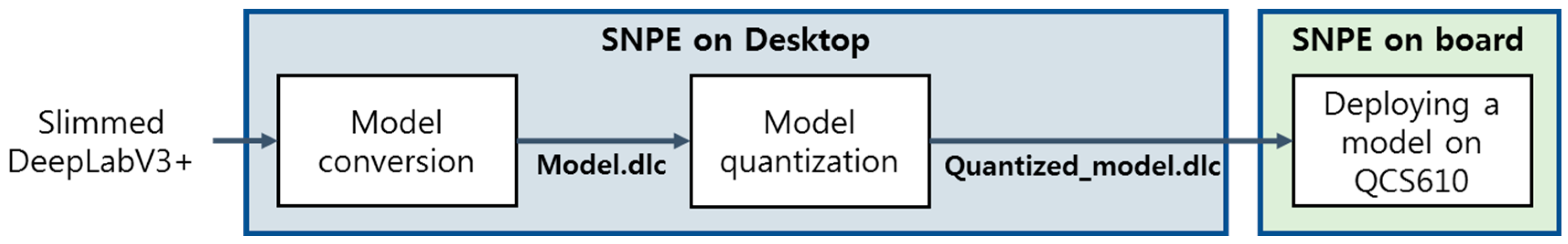
Figure 4 and Figure 5 show the process of applying network slimming to the DeepLabv3+ model to generate slimmed DeepLabv3+ and embedding the slimmed DeepLabv3+ into Qualcomm’s QCS610 chip, respectively.
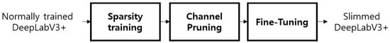
Figure 4.
Process of generating a simplified network based on the network slimming method.
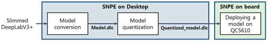
Figure 5.
Process of embedding a simplified segmentation network in QCS610.
The network slimming method used in this paper was proposed by Liu et al. [24] and consists of three steps: sparsity training, channel pruning, and fine-tuning, as shown in Figure 4. This network slimming method uses the scale parameter γ of the batch normalization layer, which is placed after the convolutional layer, as a scaling factor of the channel to determine the importance of the channel. The sparsity training step aims to make as many scaling factors go to zero as possible. This step is performed by using the loss function obtained by adding the L1 regularization term for the scaling factor to the loss function of the network, as shown in Equation (1).
In Equation (1), (x, y) is the input and target of the training data, W is the weight, the front part is the loss function of the segmentation network, the remaining part is the penalty to elicit sparsity for the scaling factor, and λ is the sparsity parameter that balances the two parts. After sparsity training, the channel pruning step determines the pruning ratio, which is the ratio of channels to be removed to the total number of channels of the network. Then, we remove the channel corresponding to the index of the scaling factor below the threshold calculated from the pruning ratio. Finally, the fine-tuning phase re-trains the parameters to fit the pruned network to obtain the final slimmed network.
In general, to deploy and operate a DNN model on an edge device, it is necessary to convert the model format to a format suitable for the embedded board environment. This is because the trained models are usually created on different deep learning frameworks, such as TensorFlow, Caffe, and PyTorch, depending on the development environment. Therefore, for embedding, we must convert our slimmed DeepLabv3+ to a format suitable for Qualcomm’s QCS610 chip. Qualcomm provides a tool called Snapdragon Neural Processing Engine (SNPE) software development kit (SDK), which provides the functions to convert models developed in different frameworks to fit on Qualcomm’s chips [25].
Deploying slimmed DeepLabv3+ on the QCS 610 chip, as shown in Figure 5, involves model conversion and quantization. In the model conversion, the file format of the model is converted into a Deep Learning Container (DLC) file, a file format available in Qualcomm chips. In this paper, we trained slimmed DeepLabv3+ in the TensorFlow framework. Therefore, we converted the model file in TensorFlow format into a DLC file suitable for Qualcomm chips using the conversion API provided by SNPE. Next is the model quantization. We run our model on the digital signal processor (DSP) of the QCS 610’s processors. The DSP on the QCS 610 is the Hexagon 685 DSP, which has a specialized architecture for AI algorithms, enabling real-time inference at low power [26]. However, the DSP only supports 8-bit integer operations. Therefore, it is essential to quantize the parameters. A quantized model is created using the quantization API provided in the SNPE SDK. Finally, embedding is completed by porting the quantized DLC file to the board [18].
3.5. Flood Warning Module
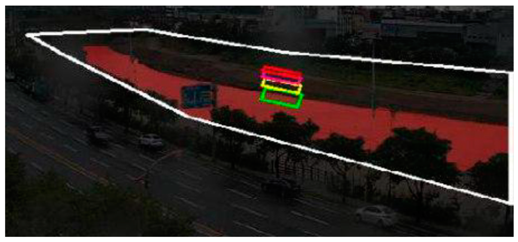
In this paper, we categorize flood warning levels into four levels: caution, alert, warning, and danger, which are predicted from the water segmentation results. We used the approach to manually set the region of interest (ROI) as in [13] and determine the flood warning level as the percentage of water area in the ROI. Figure 6 shows the ROI and small boxes needed to predict the flood warning level. First, the ROI is set as the area where the water in the river increases until it overflows in the input image. This region is marked by the white line in Figure 6. Inside this ROI, there are green, yellow, orange, and red boxes, each color representing a warning level. Green is caution, yellow is alert, orange is warning, and red is danger. The warning level is activated when the water region within each box reaches 75% or more. Our approach is more robust than methods such as those in [15,16], which only consider whether a point at a particular location is occupied within a segmented water region.

Figure 6.
ROI and four boxes for predicting flood warning levels. The color of each box indicates the warning level. Green is caution, yellow is alert, orange is warning, and red is danger.
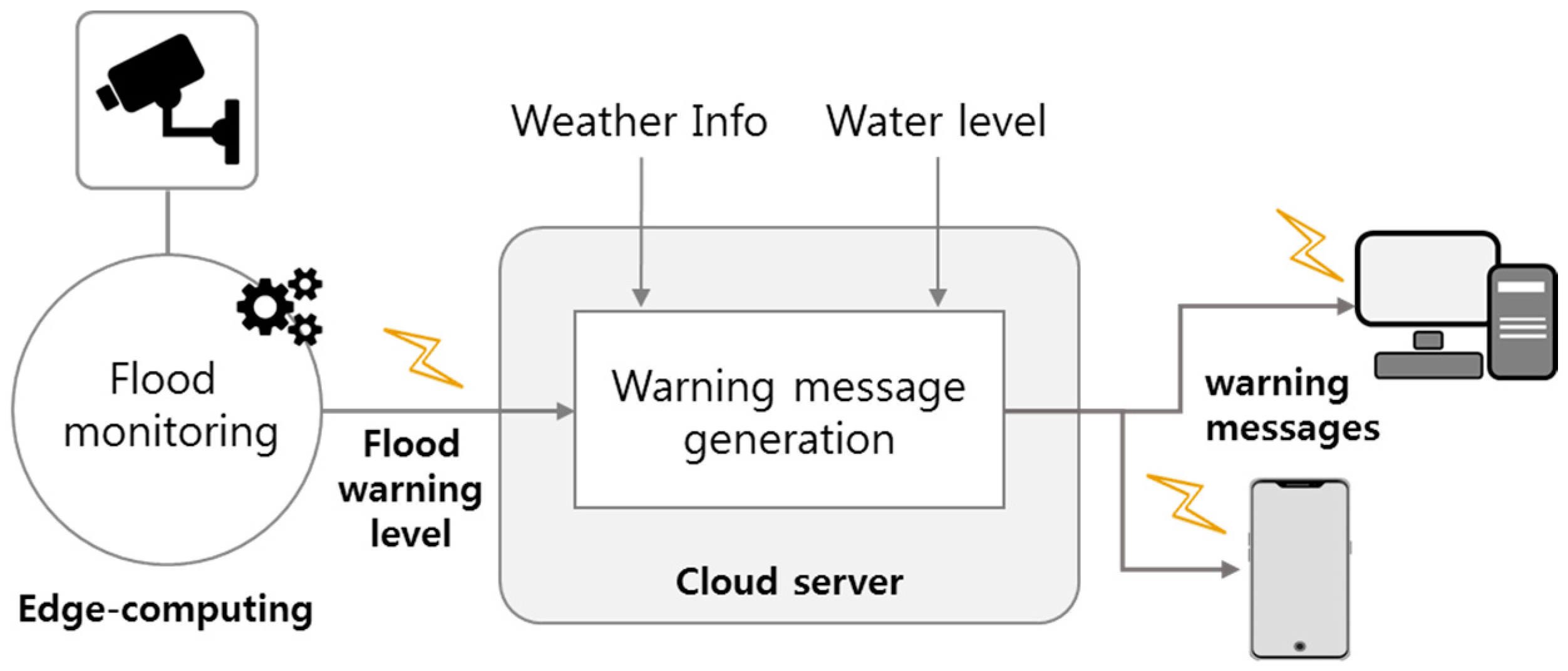
Figure 7 shows the message delivery process of the flood warning module. This module is implemented in Python, and the message includes weather and water level information along with the flood warning level. As shown in Figure 7, flood monitoring is the core process developed in this paper, which receives the images from the camera as input, processes the images on the embedded board, and outputs the flood warning level as output. The flood warning level is transmitted to the cloud server. The cloud server also receives weather information such as rainfall, wind direction, wind speed, and water level information of the reservoir near the river. By synthesizing this information, it generates a warning message for the river of interest. Warning messages are sent to authorized users’ mobile phones or PCs. Weather information is obtained using the open API of the public data portal site [27], and reservoir water level information is obtained from the Rural Agricultural Water Resource Information System [28].
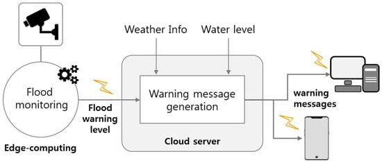
Figure 7.
Process of sending a flood warning message.
4. Experiments
4.1. Dataset
The stream where the cameras were installed to collect the dataset is shown in Figure 8. The stream has a small amount of water flowing through it during regular times, as shown in the blue region in Figure 8, but when rainfall increases, such as during the rainy season or a typhoon, the stream expands and fills in the area shown in red. The red dashed line is the boundary between the stream and the roadway on the bank. When the water of this stream crosses this boundary, flooding occurs. This stream was in fact flooded by heavy rains caused by a typhoon in September 2022. The factory and residential areas around the stream were flooded and damaged. We installed two cameras in a fixed position overlooking the stream on the roof of a building on the factory side of the stream. Each camera captures images of the stream from a different angle.
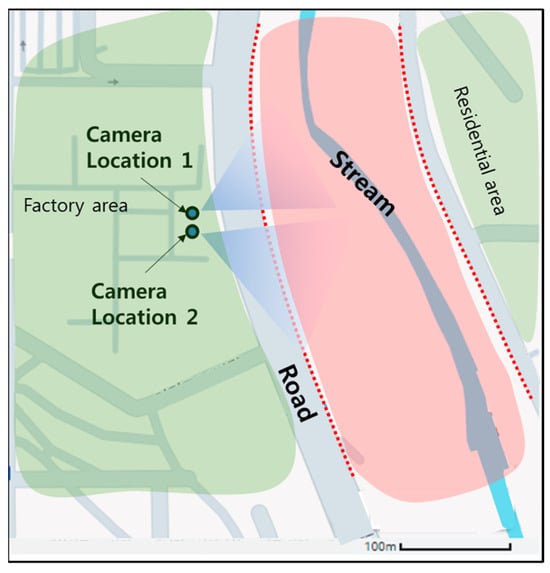
Figure 8.
Test site for flood monitoring system.
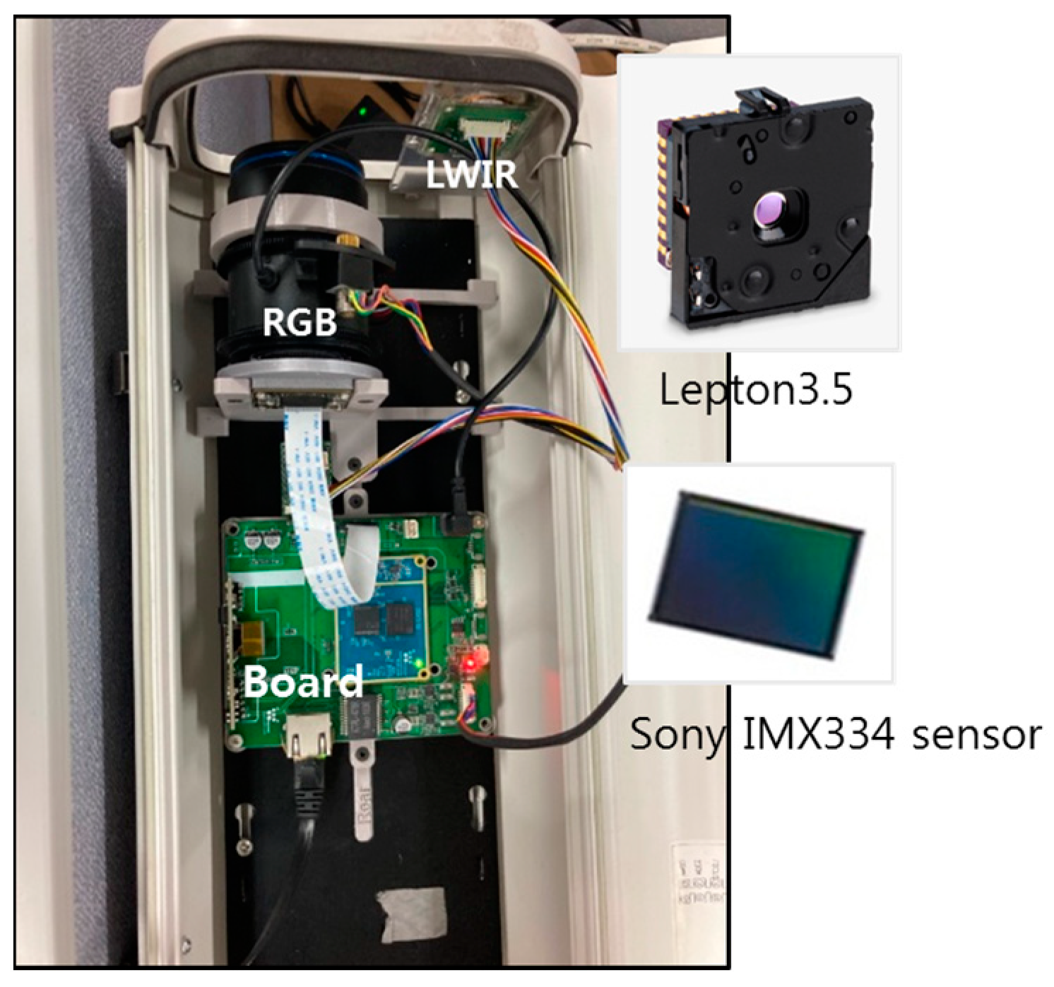
As shown in Figure 9, the camera device consists of an RGB camera, an LWIR camera, and an embedded board. The Sony IMX334 is used as the RGB sensor, and the Lepton 3.5 sensor module is used as the LWIR camera. The resolution of the RGB sensor is 3840 (H) × 2160 (V), and the resolution of the LWIR sensor is 160 (H) × 120 (V). The RGB sensor (Sony IMX334 [29]) collects visible light in the range of 400 to 700 nm wavelength and converts it into a color image. The LWIR sensor (Lepton 3.5 [30]) captures the infrared radiation in the range of 8 to 14 μm wavelength and outputs a thermal image. The embedded board has a Qualcomm QCS610 specialized for running AI algorithms.
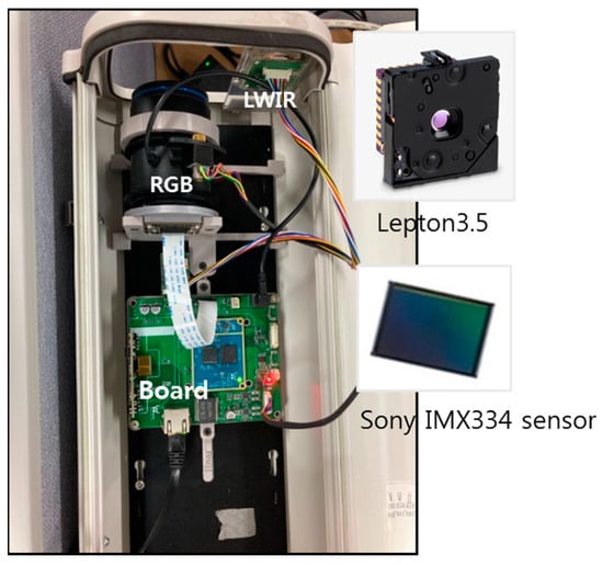
Figure 9.
Camera configuration.
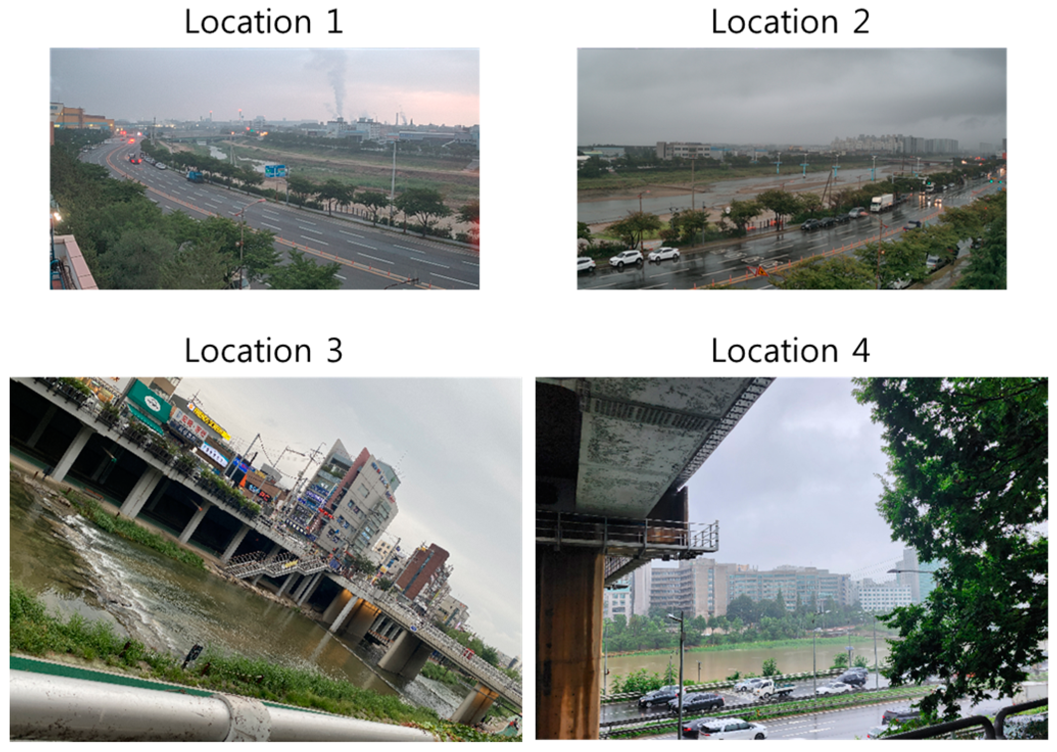
We applied two ways to collect data: using fixed cameras and using non-fixed cameras. The fixed camera method installs the cameras at Locations 1 and 2 in Figure 8 and collects data over multiple days. This is a way of collecting data considering the surveillance camera environment. The method using non-fixed cameras collects data from random locations around the river. If the network is trained with data collected only from fixed cameras, it may generate a network overfitted to a specific river shape. So, we used non-fixed cameras to collect data, including various river shapes, to avoid overfitting. The images captured by the two methods are shown in Figure 10. Image samples of Locations 1 and 2 were captured using fixed cameras. The two cameras are capturing the same stream but from different perspectives, so the location and shape of the stream appear different in the images. Locations 3 and 4 are image samples taken with a non-fixed camera around a stream and river downtown. The resolution of the non-fixed camera is 3417 (H) × 1625 (V).

Figure 10.
Examples of images collected at four different sites.
The data collection period was from 4 July to 18 September 2023, and the data include both daytime and nighttime images taken in clear, cloudy, and rainy conditions. The total number of data is 1945, and the number of data for each location and day and night data can be seen in Table 1. The data from Location 1 account for 72.4% of the total data, and the amount of daytime data is higher than that of nighttime data.

Table 1.
Distribution of data by location and number of daytime and nighttime data.
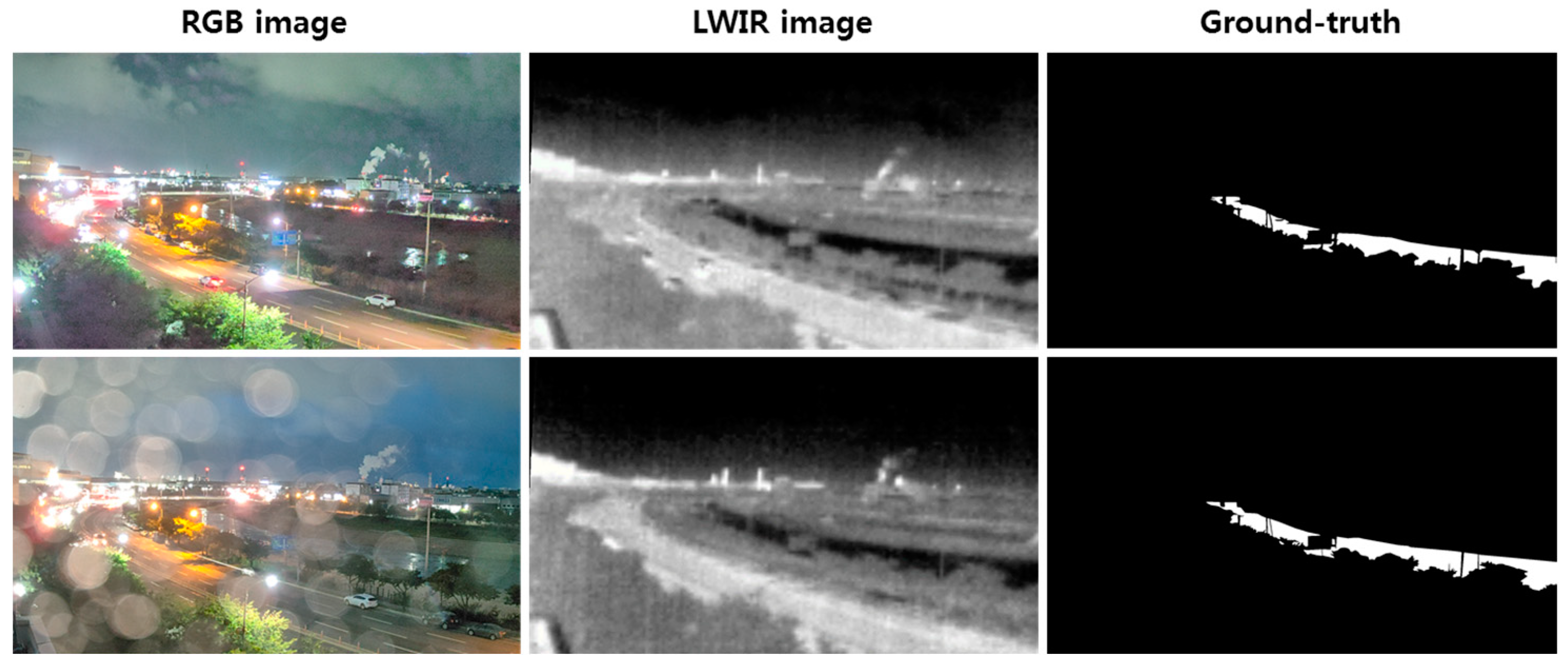
Example images for day and night are shown in Figure 11, Figure 12 and Figure 13. Each figure consists of an RGB image, an LWIR image, and a ground-truth image. The ground truth is a binary image labeled with water as one and background as zero. Figure 11 shows the daytime images, consisting of a clear weather image and a rainy weather image. Figure 12 shows the nighttime images, consisting of a clear weather image and a rainy weather image. Figure 13 shows the day and night images collected at Location 3. Compared to the daytime images in clear weather, it is challenging to distinguish water in RGB images at night or in rainy conditions because the brightness value of the image changes due to night lights or raindrops. On the other hand, in the LWIR image, the water in the river appears darker than the surrounding objects because the temperature is relatively lower than the surrounding objects. We can also find that the LWIR image is captured consistently without being significantly affected by external environmental conditions (day, night, lighting, and raindrops).
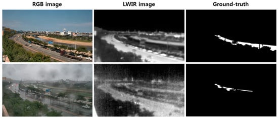
Figure 11.
Examples of daytime images.

Figure 12.
Examples of nighttime images.
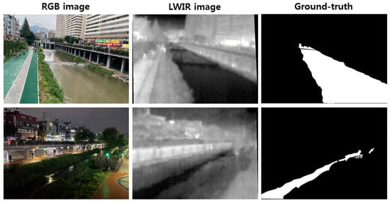
Figure 13.
Day and night images for Location 3.
4.2. Experimental Details
As shown in Table 1, the collected datasets are not evenly distributed. In other words, the images from the camera located at Location 1 account for more than 70% of the total, which means that the number of images of the same scene is quite large. Furthermore, the amount of daytime data is more significant than that of nighttime data. To prevent the semantic segmentation network from overfitting only a particular scene, we applied data augmentation to generate images with different scenes. Data augmentation generated new images using a random crop and resize method only for the images from Locations 1 and 2 using the fixed camera. Table 2 shows the data split for training, validation, and test sets. The collected datasets were separated into 1230, 268, and 447 for training, validation, and testing, respectively, and the data obtained by data augmentation consisted of 1370 images for training and 290 images for validation. After data augmentation, the total number of data is 3605, and the data distribution is approximately 70%, 15%, and 15%.
Table 2.
Data split for training, validation, and testing before and after data augmentation.
When training DeepLabv3+, the input image size was 512 (H) × 256 (V), the learning rate was 0.001, the batch size was 8, and the epoch number was 50. The additional data augmentation rate was 0.8, and data augmentation included horizontal flip, vertical flip, rotation, and zoom operations. We used the same parameter settings as normal training during sparsity training and fine-tuning in network slimming. In sparsity training, we generated five models with sparsity weights ranging from 0.001 to 100.0 in 10-fold increments. To select the model with the best sparsity training among them, we used the method of selecting the sparsity model with minor performance degradation and the highest sparsity weight value, as in [24]. The sparsity weight determined in our experiments was 1.0. For slimmed networks, we generated five models by setting the percentage of channels to be removed from the total number of channels to 50%, 60%, 70%, 80%, and 90%.
In our experiments, the performance evaluation of the segmentation network was measured by mean-over-union accuracy (mIoU). In addition, to evaluate the edge-computing potential of the slimmed model, we measured the number of parameters, the size of the model, the inference speed in frames per second (fps), and the amount of computation in GFLOPs. The inference speed of a slimmed network on the DPS of QCS 610 was calculated as the number of inferences obtained when running the network in ‘high-performance mode’ for one minute.
We conducted the experiments using two systems with the following specifications: NVIDIA TITAN RTX with 24 GB on-board memory using a Tensorflow 2.10 and Ubuntu OS installed on an Intel Core i9-10900X CPU with 64 GB RAM, and Hexagon 685 DSP using SNPE 2.12 installed on Qualcomm QCS610 SoC.
4.3. Results on the Effect of LWIR Data
To find the effect of using an LWIR camera, we compared the results of three different networks: a network using only RGB images (NRGB), a network using only LWIR images (NLWIR), and a network based on the fusion of RGB and LWIR images (NFUSION). Table 3 shows the water segmentation results of the three different networks. In the first column of the table, ‘Day’ refers to the results for images acquired during the day, ‘Night’ refers to the results for images acquired at night, and ‘Total’ refers to the results for the entire test data. From the results in Table 1, we can see three things.
Table 3.
Performance comparisons among three different networks (unit: %).
First, as we expected, NRGB performs well in the daytime with an mIoU of 90.39%, which is about 7 percentage points higher than NLWIR’s daytime result, but at night, the mIoU is 80.42%, which is significantly lower than the daytime value. This means that when using only RGB images, it is easy to segment water during the day, but at night, it is challenging to segment water accurately because it is difficult to distinguish objects.
Second, NLWIR has an mIoU of 83.77% during the day and 80.11% during the night, with relatively little difference between day and night. These results show that LWIR sensors are more robust in response to the effects of the environment because they use radiation heat information to generate images. On the other hand, the performance of NLWIR is overall lower than that of NRGB. The reason for this is that the resolution of the LWIR image is significantly smaller than that of the RGB image, so it was difficult to distinguish the shape and boundaries of the river in the LWIR image as finely as in the RGB image.
Finally, NFUSION has the highest water segmentation accuracy regardless of whether it is day or night. The mIoU is 91.00% for daytime data, 86.62% for nighttime data, and 89.80% for all datasets. In conclusion, we have demonstrated that the performance of NFUSION is much better than that of NRGB and NLWIR using a single sensor because the information between the RGB and LWIR image data is complementary, as asserted in this paper.
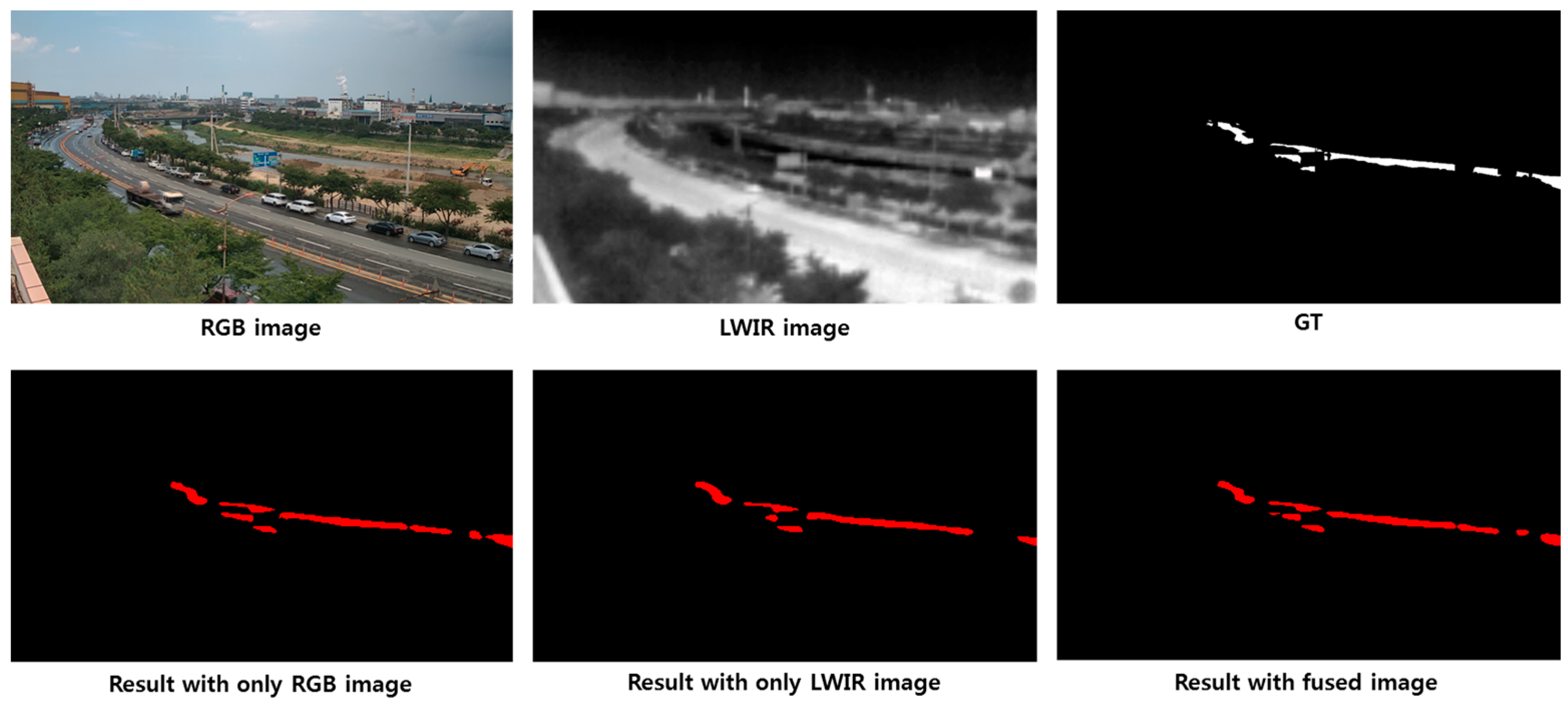
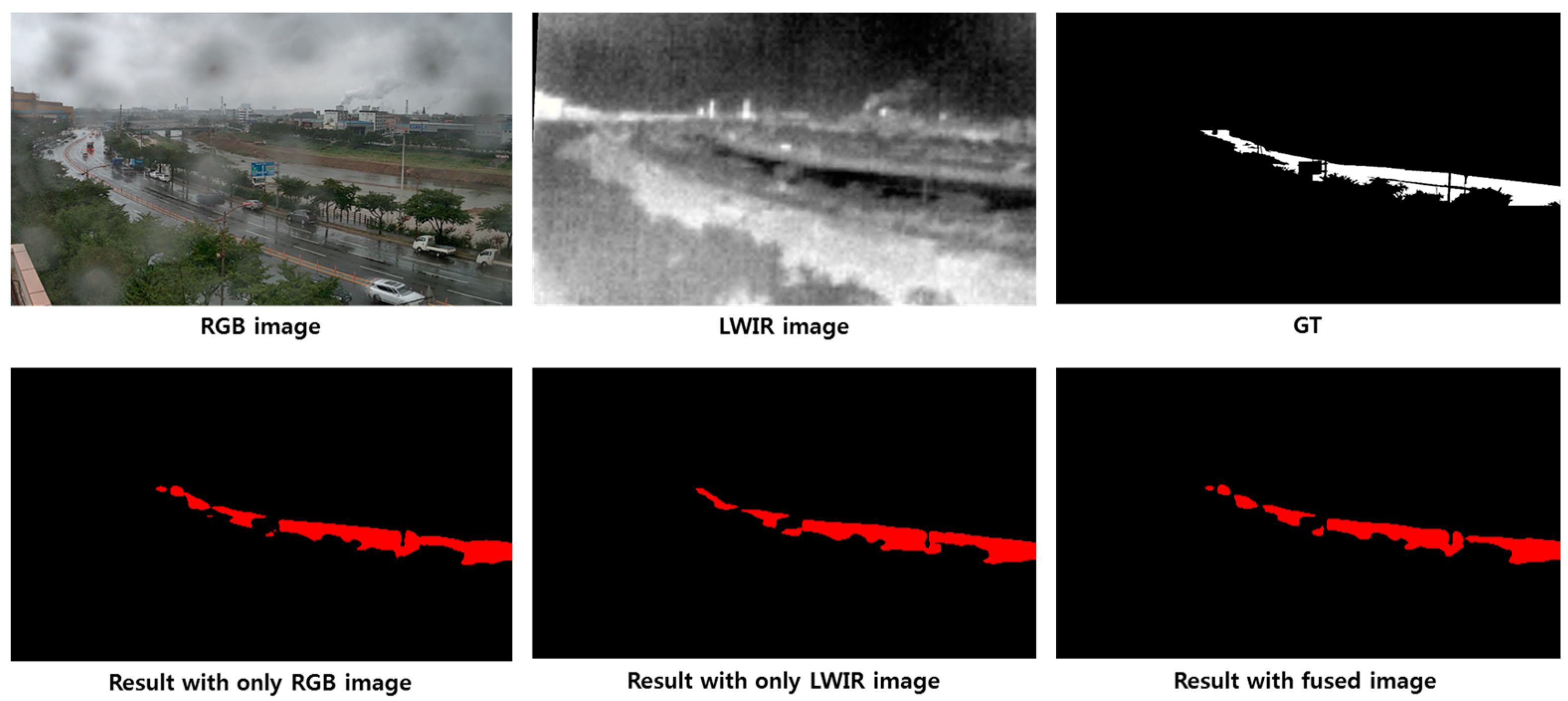
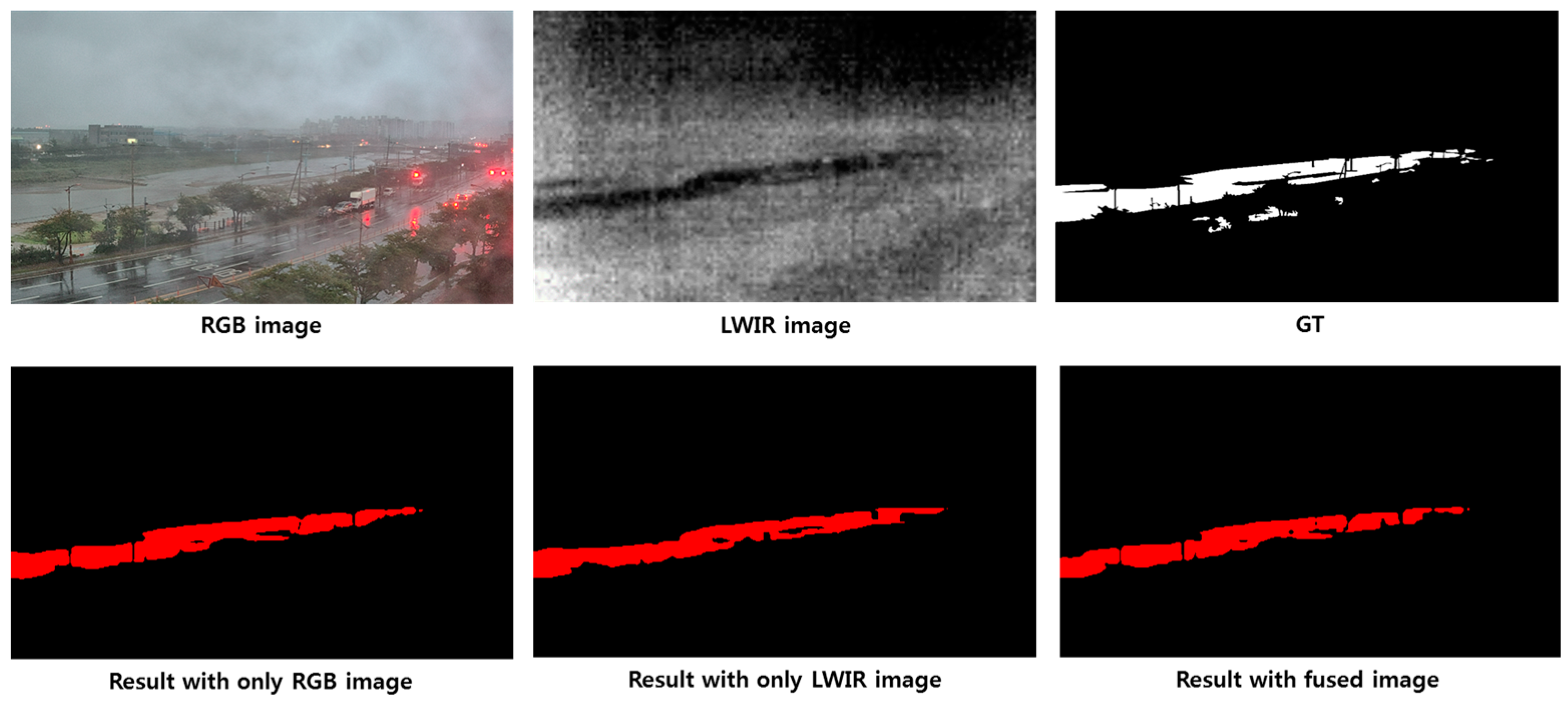
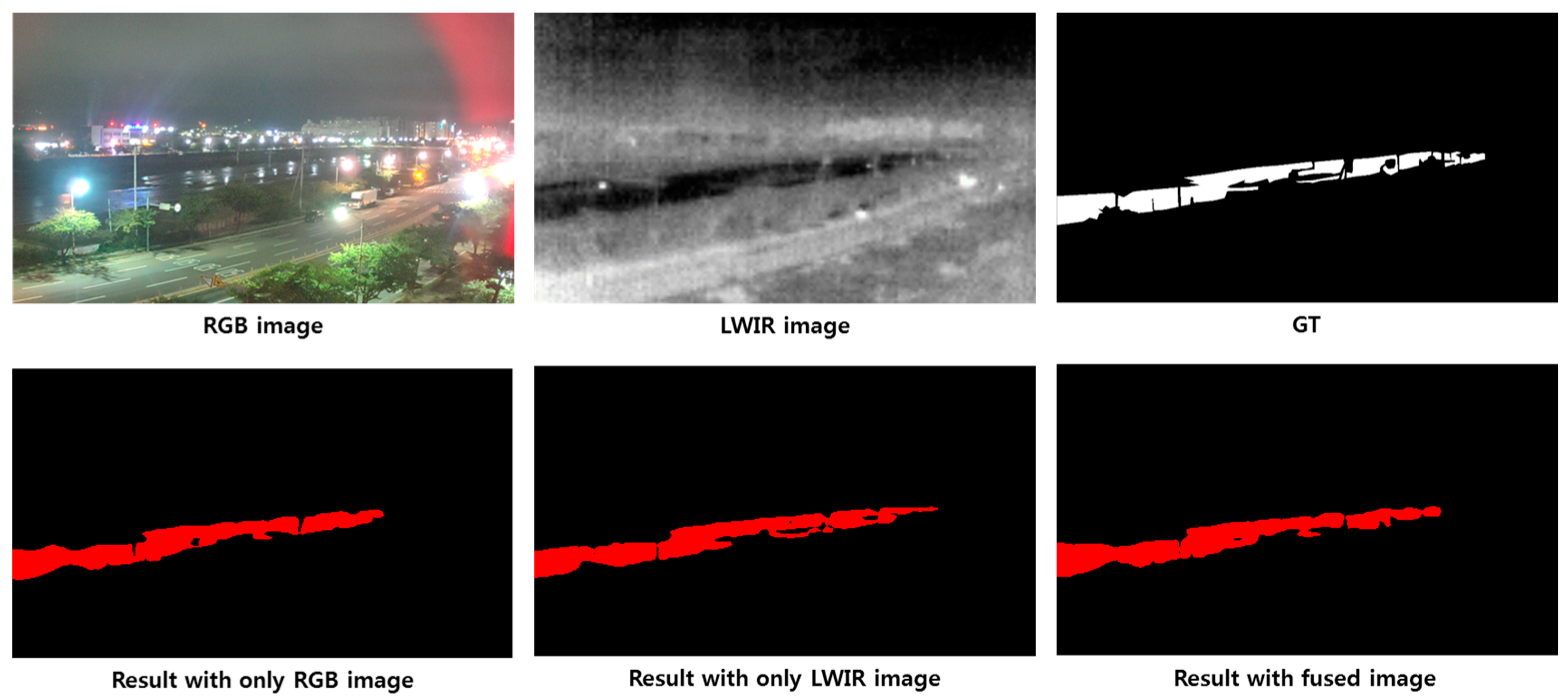
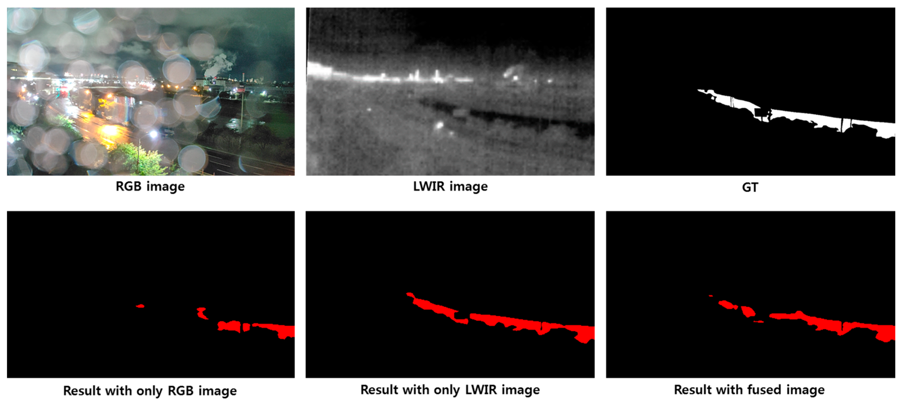
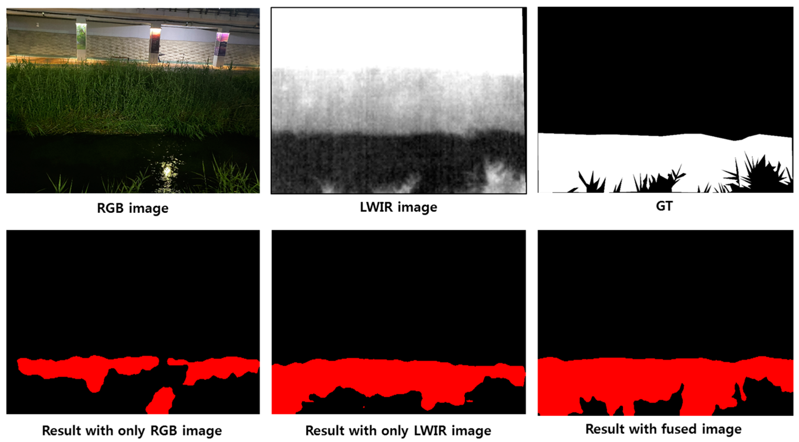
Figure 14, Figure 15, Figure 16, Figure 17, Figure 18, Figure 19 and Figure 20 show the qualitative results of NRGB, NLWIR, and NFUSION compared in different situations, such as daytime, nighttime, and rainy or clear weather. Figure 14 shows the results for the input image during the daytime in clear weather, and it can be seen that the water segmentation results of the three networks are almost similar. As shown in Figure 15 and Figure 16, we can see that the segmentation results from NLWIR and NFUSION are obtained slightly closer to the ground truth than those from NRGB because, in daytime rainy conditions, raindrops on the camera lens make it difficult to distinguish river water in RGB images. Figure 17 and Figure 18 show the results for nighttime images. In the RGB input image, it is difficult to distinguish the areas of water due to the reflection of street lights in the river or raindrops on the camera lens. However, in the LWIR image, there are no effects from streetlights or raindrops, and the river areas are easily distinguishable. The result images also show that NLWIR’s segmentation results are closer to the ground truth than the other two networks, which confirms that the LWIR sensor is robust in response to environmental changes such as nighttime and raindrops. Figure 19 and Figure 20 show images acquired at Location 3 and show results for daytime and nighttime. Figure 19 shows that the segmentation result of NFUSION is much more accurate than that of either NRGB or NLWIR. Figure 20 shows that the water segmentation result of NLWIR is more accurate than that of NRGB at night, and the segmentation result of NFUSION is more accurate than that of the other two networks.
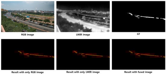
Figure 14.
Water segmentation results for an image from Location 1 during the daytime in clear weather.
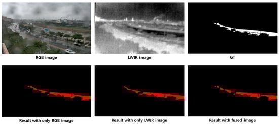
Figure 15.
Water segmentation results for an image from Location 1 during the daytime in rainy weather.
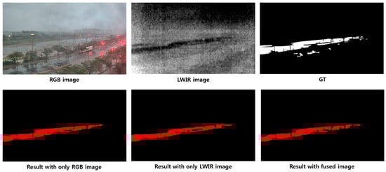
Figure 16.
Water segmentation results for an image from Location 2 during the daytime in rainy weather.
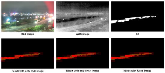
Figure 17.
Water segmentation results for an image from Location 2 during the nighttime in clear weather.
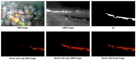
Figure 18.
Water segmentation results for an image from Location 1 during the nighttime in rainy weather.
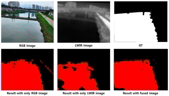
Figure 19.
Water segmentation results for an image from Location 3 during the daytime in clear weather.
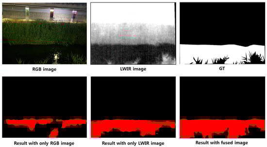
Figure 20.
Water segmentation results for an image from Location 3 during the nighttime in clear weather.
Additionally, we evaluated the proposed water segmentation network (NFUSION) under two different weather conditions: clear and rainy. In the daytime, the mIoUs for clear and rainy conditions are 90.88% and 89.38%, respectively. In the nighttime, the mIoUs for clear and rainy conditions are 86.27% and 87.44%, respectively. Since there is almost no performance difference between clear and rainy conditions, it can be said that the proposed method is robust in response to different weather conditions.
4.4. Results on Edge Device
Table 4 shows the segmentation results of the slimmed networks according to the pruning ratio after the application of network slimming to the DeepLabv3+ model based on RGB and LWIR sensor fusion. The pruning ratio ranges from 50% to 90%. In this table, ‘Baseline’ means the performance of normally trained DeepLabv3+. The experimental results show that there is little performance degradation when the pruning ratio is from 50% to 70%. However, the performance of the slimmed network drops sharply when the pruning ratio is more than 80%. In this paper, in order to reduce the size of the network as much as possible with slight performance degradation, we selected the 70% pruned network as the final one and ported it to the Qualcomm QCS610 SoC to measure the performance.
Table 4.
Performance comparisons among the slimmed networks created according to pruning ratio (unit: %).
Table 5 shows the performance of the baseline and slimmed networks as measured by QCS 610. Table 5 compares the two networks’ accuracy, memory capacity, inference speed, and the amount of computation. The mIoU for the baseline is 89.64%, while the mIoU for slimmed_70 (the network with 70% of the channels removed) is 89.72%. The accuracies of the two networks are almost identical. However, the size and number of parameters in the slimmed network are about ten times smaller than those in the baseline, and the amount of computation is about three times smaller. In addition, if the baseline runs on a DSP, it obtains inference results at a speed of 1 frame per second. On the other hand, slimmed_70 obtains water segmentation results at a speed of 12 frames per second. These results demonstrate that the proposed system has the potential to perform real-time water segmentation with the same high accuracy as large-scale networks with less computation and less memory in real-world flood monitoring systems.
Table 5.
Performance comparisons between the baseline network and 70% slimmed network on DSP of QCS 610.
4.5. Results for Warning Message
Figure 21 shows the actual screen of the warning message sent to the smartphone app and the computer program. In our module, warning messages are created after the predicted flood warning level is delivered to the flood warning system. Figure 21a is a screen capture of the smartphone app, and Figure 21b is a screen capture of the PC program. In practice, flood monitoring was performed on fixed cameras installed at Locations 1 and 2 for the surveillance camera scenario.
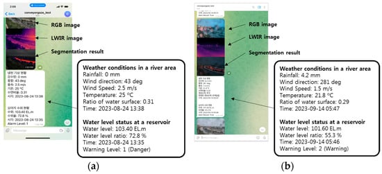
Figure 21.
Example images for the results of sending warning messages: (a) example on smartphone app; (b) example on PC program.
The message contents are as follows: Firstly, the RGB and LWIR images from the camera are sent, followed by the water segmentation result. The message includes the weather status, water level status, and flood warning level. The weather status consists of information about the stream area, including rainfall, wind direction, wind speed, temperature, water surface ratio, and time. Water level status shows the level of a reservoir near the stream. The purpose of using this information is to analyze the correlation between the water level in the reservoir and the flood warning level of the stream. The water level status consists of the water level, water level rate, time, and warning level. Figure 21a shows a warning level 1 (danger) message sent when a stream rose in August. Figure 21b shows a warning level 2 (warning) message sent when the stream rose after a rainy event.
The message-sending module operated from late August through October. There was one flood risk event in August due to heavy rainfall, but the remaining months were mostly dry, so we were not able to verify the accuracy of the flood risk prediction. However, we did see that messages were successfully sent for more than two months, as shown in Figure 21.
5. Conclusions
This paper proposes a DNN-based flood monitoring system fusing RGB and LWIR surveillance cameras for edge devices. The RGB and LWIR sensor fusion enables 24 h flood monitoring regardless of whether it is day or night. The experimental results showed that the fusion of RGB and LWIR images improved water segmentation accuracy over using a single sensor alone. We also showed that combining AI and edge computing in surveillance cameras can enable real-time monitoring for various applications, including flood monitoring, pedestrian or vehicle surveillance, and more. To create a simplified network, we used the network slimming method and obtained meaningful results by deploying the lightweight network on a Qualcomm QCS610 and performing network inference. The experimental results showed that the network slimming method increased the inference speed of the network by 12 times, reduced the model size by 10 times, and reduced the number of computations by 3 times without any performance degradation. Finally, the flood warning level was detected from the water segmentation results obtained by DeepLabv3+. The warning level was sent to a smartphone or personal computer through the message generation module implemented in this paper.
This study has implemented all the elements practically required in a surveillance-camera-based flood monitoring system and demonstrated the potential of each element to be utilized in a flood monitoring system through experimental results. However, there is still much more work to be conducted. In future work, we plan to test and improve the proposed system for a few more years while increasing the dataset at more sites to obtain a quantitative result with detailed accuracy on the warning level. And we plan to study how to apply a dual encoder network to fuse RGB and LWIR images to enhance the effectiveness of the fusion further and improve the network’s performance. We also plan to apply the proposed system to the monitoring of fire, a disaster as common as flooding.
Author Contributions
Conceptualization, Y.J.L., H.G.J. and J.K.S.; methodology, Y.J.L., J.Y.H., J.P., H.G.J. and J.K.S.; software, Y.J.L., J.Y.H. and J.P.; validation, Y.J.L., J.Y.H., J.P., H.G.J. and J.K.S.; formal analysis, Y.J.L., H.G.J. and J.K.S.; investigation, Y.J.L.; resources, Y.J.L., J.Y.H. and J.P.; data curation, Y.J.L. and J.Y.H.; writing—original draft preparation, Y.J.L.; writing—review and editing, H.G.J. and J.K.S.; visualization, Y.J.L.; supervision, H.G.J. and J.K.S.; project administration, J.K.S.; funding acquisition, J.K.S. All authors have read and agreed to the published version of the manuscript.
Funding
This work was supported in part by WITHROBOT, and in part by the Basic Science Research Program through the National Research Foundation of Korea (NRF) funded by the Ministry of Education (2020R1A6A1A03038540).
Data Availability Statement
Data are contained within the article.
Conflicts of Interest
The authors declare no conflicts of interest.
References
- Khan, A.; Gupta, S.; Gupta, S.K. Multi-hazard disaster studies: Monitoring, detection, recovery, and management, based on emerging technologies and optimal techniques. Int. J. Disaster Risk Reduct. 2020, 47, 101642. [Google Scholar] [CrossRef]
- Khan, A.; Gupta, S.; Gupta, S.K. Emerging UAV technology for disaster detection, mitigation, response, and preparedness. J. Field Robot. 2022, 39, 905–955. [Google Scholar] [CrossRef]
- UNDRR. The Human Cost of Disasters—An Overview of the Last 20 Years 2000–2019; UNDRR: Geneva, Switzerland, 2020. [Google Scholar]
- Anbarasan, M.; Muthu, B.; Sivaparthipan, C.B.; Sundarasekar, R.; Kadry, S.; Krishnamoorthy, S.; Samuel, R.D.; Dasel, A.A. Detection of flood disaster system on IoT, big data and convolutional deep neural network. Comput. Commun. 2020, 150, 150–157. [Google Scholar] [CrossRef]
- Prakash, C.; Barthwal, A.; Acharya, D. FLOODWALL: A Real-Time Flash Flood Monitoring and Frecasting System Using IoT. IEEE Sens. J. 2023, 23, 787–799. [Google Scholar] [CrossRef]
- Chowdhury, T.; Rahnemoonfar, M.; Murphy, R.; Fernandes, O. Comprehensive Semantic Segmentation on High Resolution UAV imagery for Natural Disaster Damage Assessment. In Proceedings of the 2020 IEEE International Conference on Big Data, Atlanta, GA, USA, 10–13 December 2020. [Google Scholar]
- Hernández, D.; Cecilia, J.M.; Cano, J.C.; Calafate, C.T. Flood Detection Using Real-Time Image Segmentation from Unmanned Aerial Vehicles on Edge-Computing Platform. Remote Sens. 2022, 14, 223. [Google Scholar] [CrossRef]
- Puspitasri, R.D.; Annisa, F.Q.; Ariyanto, D. Flooded Area Segmentation on Remote Sensing Image from Unmanned Aerial Vehicles (UAV) using DeepLabV3 and EfficientNet-B4 Model. In Proceedings of the 2023 International Conference on Computer, Control, Informatics and Its Applications, Bandung, Indonesia, 4–5 October 2023; pp. 216–220. [Google Scholar]
- Basnyat, B.; Roy, N.; Gangopadhyay, A. Flood Detection using Semantic Segmentation and Multimodal Data Fusion. In Proceedings of the 6th IEEE International Workshop on Pervasive Context-Aware Smart Cities and Intelligent Transport System, Kassel, Germany, 22–26 March 2021; pp. 135–140. [Google Scholar]
- Lopez-Fuentes, L.; Rossi, C.; Skinnemoen, H. River segmentation for flood monitoring. In Proceedings of the 2017 IEEE International Conference on Big Data, Boston, MA, USA, 11–14 December 2017; pp. 3746–3749. [Google Scholar]
- Baydargil, H.B.; Park, J.; Shin, H.S.; Park, K. Water Flow Detection Using Deep Convolutional Encoder-decoder Architecture. In Proceedings of the 2018 18th International Conference on Control, Automation and Systems, PyeongChang, Republic of Korea, 17–20 October 2018; pp. 841–843. [Google Scholar]
- Akiyama, T.S.; Marçato Junior, J.; Goncalves, W.N.; Bressan, P.O.; Eltner, A.; Binder, F.; Singer, T. Deep Learning Applied to Water Segmentation. Int. Arch. Photogramm. Remote Sens. Spat. Inf. Sci. 2020, XLIII-B2-2020, 1189–1193. [Google Scholar]
- Vitry, M.M.; Kramer, S.; Wegner, J.D.; Leitão, J.P. Scalable flood level trend monitoring with surveillance cameras using a deep convolutional neural network. Hydrol. Earth Syst. Sci. 2019, 23, 4621–4634. [Google Scholar] [CrossRef]
- Borwarninginn, P.; Haga, J.H.; Kusakunniran, W. Water Level Detection from CCTV Cameras using a Deep Learning Approach. In Proceedings of the 2020 IEEE Region 10 Conference, Osaka, Japan, 16–19 November 2020; pp. 1283–1288. [Google Scholar]
- Vandaele, R.; Dance, S.L.; Ojha, V. Automated Water Segmentation and River Level Detection on Camera Images Using Transfer Learning. Pattern Recognit. 2021, 12544, 232–245. [Google Scholar]
- Muhadi, N.A.; Abdullah, A.F.; Bejo, S.K.; Mahadi, M.R.; Mijic, A. Deep Learning Semantic Segmentation for Water Level Estimation Using Surveillance Camera. Appl. Sci. 2021, 11, 9691. [Google Scholar] [CrossRef]
- Fernandes Junior, F.E.; Nonato, L.G.; Ranieri, C.M. Memory-Based Pruning of Deep Neural Networks for IoT Devices Applied to Flood Detection. Sensors 2021, 21, 7506. [Google Scholar] [CrossRef] [PubMed]
- Lee, Y.J.; Jung, H.G.; Suhr, J.K. Semantic Segmentation Network Slimming and Edge Deployment for Real-time Forest Fire or Flood Monitoring System Using Unmanned Aerial Vehicles. Electronics 2023, 12, 4795. [Google Scholar] [CrossRef]
- Hartley, R.; Zisserman, A. Multiple View Geometry in Computer Vision, 2nd ed.; Cambridge University Press: Cambridge, UK, 2004; p. 36. [Google Scholar]
- Chen, L.-C.; Zhu, Y.; Papandreou, G.; Schroff, F.; Adam, H. Encoder-Decoder with Atrous Separable Convolution for Semantic Image Segmentation. In Proceedings of the European Conference on Computer Vision (ECCV), Munich, Germany, 8–14 September 2018; pp. 801–818. [Google Scholar]
- Chen, L.; Papandreou, G.; Kokkinos, I.; Murphy, K.; Yuille, A.L. Semantic Image Segmentation with Deep Convolutional Nets and Fully Connected CRFs. arXiv 2014, arXiv:1412.7062. [Google Scholar]
- Chen, L.; Papandreou, G.; Kokkinos, I.; Murphy, K.; Yuille, A.L. DeepLab: Semantic Image Segmentation with Deep Convolutional Nets, Atrous Convolution, and Fully Connected CRFs. IEEE Trans. Pattern Anal. Mach. Intell. 2018, 40, 834–848. [Google Scholar] [CrossRef] [PubMed]
- Chen, L.; Papandreou, G.; Schroff, F.; Adam, H. Rethinking Atrous Convolution for Semantic Image Segmentation. arXiv 2017, arXiv:1706.05587v3. [Google Scholar]
- Liu, Z.; Li, J.; Shen, Z.; Huang, G.; Yan, S.; Zhang, C. Learning Efficient Convolutional Networks through Network Slimming. In Proceedings of the 2017 IEEE International Conference on Computer Vision, Venice, Italy, 22–29 October 2017; pp. 2755–2763. [Google Scholar]
- Qualcomm Neural Processing SDK. Available online: https://developer.qualcomm.com/software/qualcomm-neural-processing-sdk (accessed on 8 April 2024).
- Qualcomm Hexagon 685 DSP Is a Boon for Machine Learning. Available online: https://www.xda-developers.com/qualcomm-snapdragon-845-hexagon-685-dsp/ (accessed on 8 April 2024).
- Public Data Portal. Available online: https://www.data.go.kr/en/index.do (accessed on 8 April 2024).
- Rural Agricultural Water Resource Information System. Available online: https://rawris.ekr.or.kr/main.do (accessed on 8 April 2024).
- Sony IMX334. Available online: https://www.framos.com/wp-content/uploads/FSM-IMX334-Datasheet.pdf (accessed on 17 June 2024).
- Lepton 3.5 Module. Available online: https://www.flir.eu/products/lepton/?model=500-0771-01&vertical=microcam&segment=oem (accessed on 17 June 2024).


Disclaimer/Publisher’s Note: The statements, opinions and data contained in all publications are solely those of the individual author(s) and contributor(s) and not of MDPI and/or the editor(s). MDPI and/or the editor(s) disclaim responsibility for any injury to people or property resulting from any ideas, methods, instructions or products referred to in the content. |
© 2024 by the authors. Licensee MDPI, Basel, Switzerland. This article is an open access article distributed under the terms and conditions of the Creative Commons Attribution (CC BY) license (https://creativecommons.org/licenses/by/4.0/).