Abstract
In recent years, deep learning-based classification methods for hyperspectral images (HSIs) have gained widespread popularity in fields such as agriculture, environmental monitoring, and geological exploration. This is owing to their ability to automatically extract features and deliver outstanding performance. This study provides a new Dilated Spectral–Spatial Gaussian Transformer Net (DSSGT) model. The DSSGT model incorporates dilated convolutions as shallow feature extraction units, which allows for an expanded receptive field while maintaining computational efficiency. We integrated transformer architecture to effectively capture feature relationships and generate deep fusion features, thereby enhancing classification accuracy. We used consecutive dilated convolutional layers to extract joint low-level spectral–spatial features. We then introduced Gaussian Weighted Pixel Embedding blocks, which leverage Gaussian weight matrices to transform the joint features into pixel-level vectors. By combining the features of each pixel with its neighbouring pixels, we obtained pixel-level representations that are more expressive and context-aware. The transformed vector matrix was fed into the transformer encoder module, enabling the capture of global dependencies within the input data and generating higher-level fusion features with improved expressiveness and discriminability. We evaluated the proposed DSSGT model using five hyperspectral image datasets through comparative experiments. Our results demonstrate the superior performance of our approach compared to those of current state-of-the-art methods, providing compelling evidence of the DSSGT model’s effectiveness.
1. Introduction
Hyperspectral techniques are crucial instruments used to gather and analyse continuous spectrum data on objects in various wavelength ranges. In addition to offering a wide area for the advancement of hyperspectral image (HSI) classification study, the diverse and rich methods of acquiring hyperspectral data also present new problems and opportunities for our comprehension and use of hyperspectral data. HSIs are currently used in several industries, including food safety [1,2], medical diagnostics [3], industrial product quality inspection [4], mineral detection [5], and pest and disease monitoring [6]. A wide range of topics, including noise removal [7], spectrum unmixing [8], data classification and clustering [9], and target identification and recognition [10,11], have been covered by the rich and varied development of HSI processing approaches.
Feature land cover classification algorithms are challenged by the complex spectral properties and high-dimensional features of hyperspectral data. Programs such as Spectral Angle Mapper [12], Support Vector Machines [13,14], Decision Tree [15], and K-Nearest Neighbours [16] identified HSI in the first stage of the process based solely on the similarity or difference between their spectra. In situations when there is a considerable amount of spectral overlap or similarity, techniques that solely consider spectral features have not worked effectively. Therefore, efforts have been made to solve this issue using techniques such as the extended multi-attribute profile (EMAP) [17], the grey scale covariance matrix (GLCM) [18] based on texture features, and the morphological profile (MP) [19] based on shape features. These techniques for logically fusing and representing spectral and spatial characteristics can be used to acquire pixel features that are more thorough and precise. To increase the effectiveness and efficiency of classification, HSIs typically require various dimensionality reduction techniques, such as principal component analysis (PCA) [20,21] and linear discriminant analysis (LDA) [22,23], to maintain important data dimensions and features.
Traditional classification methods often require manual feature selection. The quality and effectiveness of feature extraction rely heavily on human experience and domain knowledge, which may not fully capture the complex and abstract features in images. In comparison, deep learning-based classification methods have stronger feature learning capabilities and automated feature extraction abilities. In this context, they have demonstrated strong performance in the field of image processing tasks. Various HSI classification methods have been proposed based on convolutional neural networks (CNNs) [9,24,25,26,27,28,29,30,31,32,33]. Although CNN-based networks have achieved positive results in visual classification, some areas require optimisation. CNNs typically require a large amount of training data, and smaller datasets may not be sufficient to fully train the CNN model, leading to overfitting. Given the complexity and large number of parameters in CNNs, the training time can be relatively long. The receptive field obtained by CNNs is strongly influenced by the size and variations in the input data. In the context of high-dimensional data such as hyperspectral images, traditional CNN models may require dimensionality reduction or the decomposition of spectral data to adapt to the input requirements of the model.
To address these issues raised regarding CNNs, such as parameter redundancy and a limited ability to handle spatial and scale variations, researchers have introduced various CNN variants to improve the models and enhance the performance and adaptability of CNNs. Wang et al. [34] proposed a model known as the expansion spectral–spatial attention network. It introduces expansion convolution as a dual-branch feature extraction unit, which expands the receptive field of input patches, enhancing the perception of large-scale features. In Ref. [35], kernel-guided deformable convolution was used to dynamically adjust the sampling positions of the convolution kernel, extracting pure spatial–spectral information from the local neighbourhood. Zhao et al. [36] presented a grouped separable convolution model, which combines grouped convolution and separable convolution to reduce the number of parameters and improve computational efficiency. By introducing different convolution operations and sampling mechanisms, these CNN variants effectively increase the receptive field range of the model and more effectively capture spectral, structural, textural, and spatial shape information in images without introducing extra parameters. They also reduce the number of parameters and computational complexity in the network, allowing the model to maintain efficient performance even in resource-constrained environments.
HSI data typically contain many spectral bands, where certain bands are more important for classification tasks and others may contain noise or redundant information. Attention mechanisms [37,38,39,40,41] can assist models to automatically learn and focus on crucial features. The introduction of Vision Transformer [42,43,44,45,46] has opened new avenues for attention-based model design. Visual Transformers use multi-head self-attention mechanisms (MHSAs) and feedforward neural networks for feature extraction instead of CNNs. Through MHSAs, transformers can globally model the relationships within the entire input sequence, enabling more effective capturing of global dependencies in images. Each MHSA head can focus on different correlations, allowing transformers to learn richer and more diverse feature representations. In contrast, relying solely on CNNs for feature representation is limited by fixed convolution kernels and pooling operations. This may fail to capture diverse features within the input. Many researchers have successfully combined transformers with other components of CNNs, achieving state-of-the-art results in image classification tasks [47,48,49,50,51,52].
However, the visual transformer was originally designed for RGB natural images, and applying the transformer to HSI classification tasks still has multiple challenges. Although the transformer has certain advantages in processing images with fewer channels, when dealing with HSIs, which have multiple spectral bands, there may be issues with scattered feature extraction. HSI data have a larger number of spectral bands for each pixel, and the multi-head self-attention (MHSA) in the transformer may establish long-range dependency correlations on a global scale, thereby excluding the local spatial relationships between pixels. This research offers Dilated Spectral–Spatial Gaussian Transformer Net (DSSGT) as a new model framework to enhance transformer performance on HSI classification tasks. The low-level null-spectrum joint characteristics of the input data were extracted using a two-branch cascade of dilated convolutional layers. By using this tactic, the receptive field for global information could be expanded, while the computing burden was decreased. The low-level joint features were then transformed into pixel-level vectors using a Gaussian weight matrix. This was then fed into the transformer encoder block to create high-level long-range fusion features. By using global average pooling to predict the labels of each pixel, we created a classification map.
A summary of the key contributions of this study includes the following:
(1) We proposed a low-level feature extraction module based on dilated convolution. This module stacks multiple dilated convolution layers with different dilation rates to perceive dependencies between features at different scales, thereby enlarging the receptive field and aggregating the obtained features. This allowed us to capture broader spatial–spectral contextual information and global structural correlations while also reducing computational complexity.
(2) We designed a Gaussian Weighted Pixel Embedding block that transforms low-level fusion features into pixel-level vector representations by introducing Gaussian weighted encoding. This transformation method enables the generation of more expressive and context-aware vector matrices, thereby enhancing the representation capability of the features.
(3) By combining a Dilated Convolutional Feature Extraction Unit and a Transformer Architecture Feature Fusion Unit, low, mid, and high semantic HSI features can be extracted effectively and efficiently, and more expressive and discriminative feature representations can be created. Five datasets were the subject of extensive study to verify the efficacy of the suggested model.
2. Methodology
2.1. DSSGT Framework
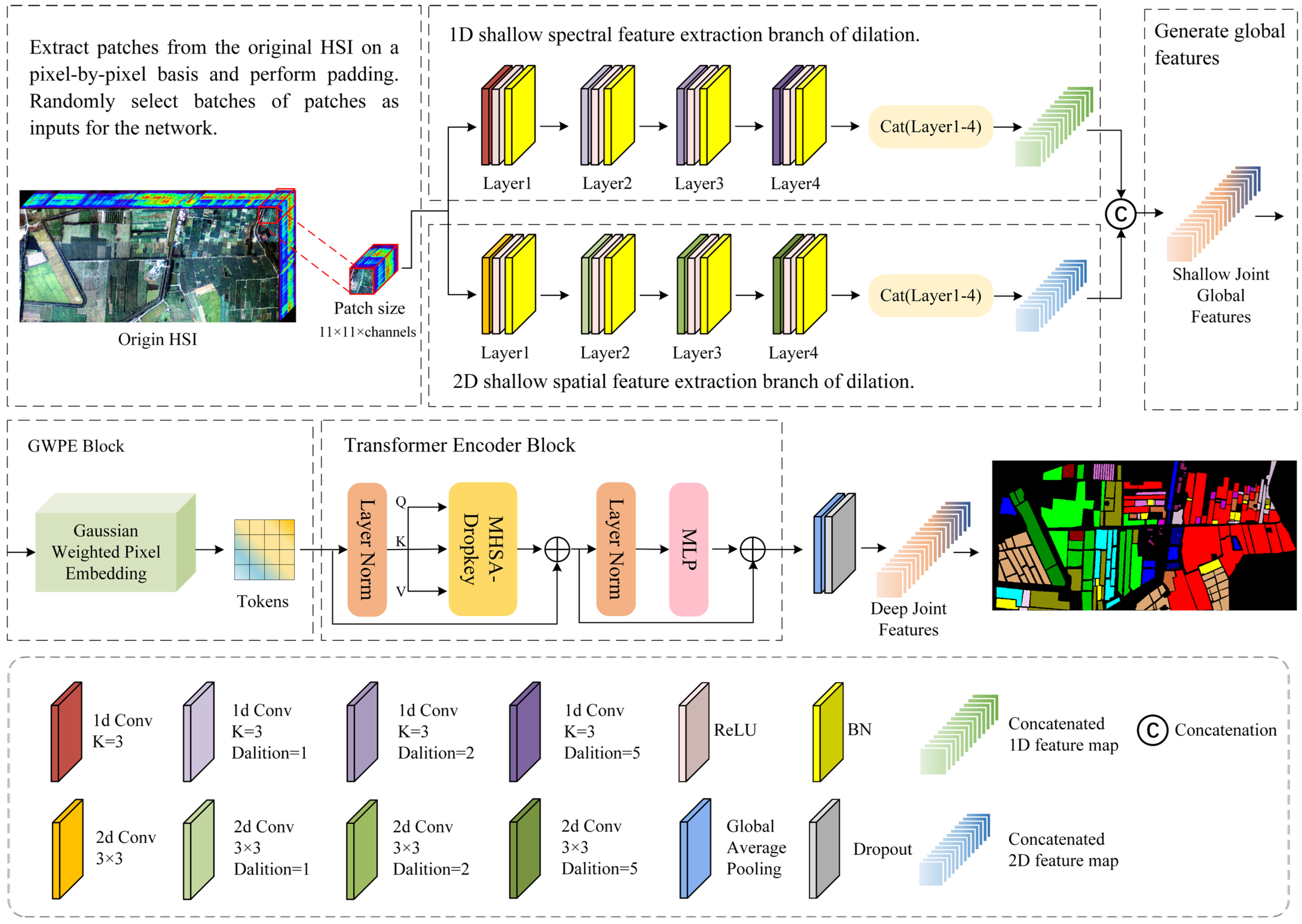
Figure 1 shows the entire framework overview diagram for the DSSGT model. The two model components include a shallow backbone for extracting spatial–spectral features based on dilated convolutional neural networks and a deep backbone for fusing features based on the transformer and GGWPE. Dilation convolution expands the sense field in comparison to regular convolution by introducing fixed-spaced zero-valued items into the convolution kernel. By expanding the convolutional kernel’s effective receptive field, this method can be used to collect a larger variety of spatial–spectral contextual information. The double branches, or the spatial branch and the spectral branch, based on dilated convolutional layers, are used by the shallow spatial–spectral feature extraction backbone of DSSGT to extract HSI features. Among these, the spectral and spatial branches extract effective information in the HSI through one-dimensional and two-dimensional dilatational convolution, respectively. By providing a Gaussian weight function that gives greater weight to the neighbouring points around each feature point in the feature space to more effectively capture the correlation and local structure between features, the GWPE block improves the accuracy of feature representation.
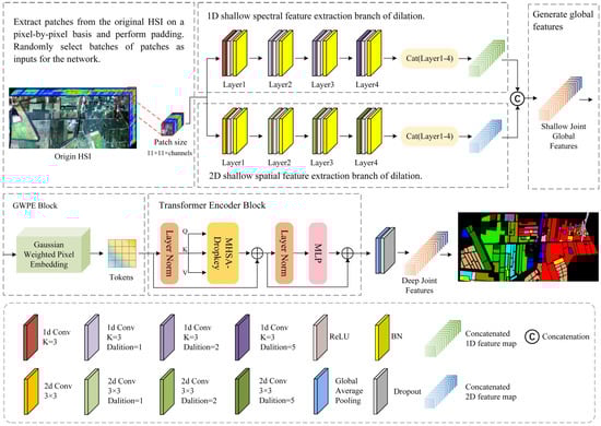
Figure 1.
Detailed flowchart of the DSSGT model.
We extracted an image block in both height and width dimensions that was centred on each pixel point in the HSI. We then used a two-branch network to extract the spatial and spectral properties of this image block independently. To ensure that the ensemble features supplied to the deep feature fusion backbone encompassed all the recovered shallow information, we stitched the output feature maps of the four dilated convolutional layers in each branch (Layers 1–4). To produce more representative feature embedding, the Gaussian weighting function in GWPE can be adaptively modified by the distribution of features in the space. For us to generate a suitable embedding representation for the input transformer, we first needed to process the ensemble features through the GWPE block. The deep feature fusion information could only then be extracted through the transformer encoder block. We created the classification graph by mapping characteristics to matching category labels using global average pooling across categories.
We separated the sample data into a training set, a validation set, and a test set, each playing a different role in the study. The training set played a crucial role in model parameter learning and training. By training the model on the training set, we gradually learned and adjusted the weights and parameters of the model to better fit the features and patterns of the training data. The validation set was used for model tuning and hyperparameter selection. The test set was used to evaluate the performance and generalisation ability of the trained model. The proper partitioning and use of these three datasets formed the foundation for ensuring the reliability, generalisation ability, and effectiveness of the model.
2.2. Shallow Feature Extraction Backbone
2.2.1. Convolution of One- and Two-Dimensional Dilation
The size of the region in the input feature map that a convolutional layer concentrates on is determined by the size of the convolutional kernel of the layer below. The performance and expressiveness of the neural network strongly depend on the size of the receptive field, with larger receptive fields capable of capturing a wider range of contextual data. Therefore, a broader receptive field offers a more detailed perspective and aids in a deeper understanding and recognition of the input information while processing images containing large-scale elements. By enlarging the convolution kernel, ordinary convolution often expands the receptive field. However, this increases the number of parameters and the computational complexity, which could cause model overfitting. In practical applications, we need to strike a balance between the size of the receptive field and the constraints of computational resources. To achieve this, additional methods, such as dilation convolution, can be used in combination to widen the receptive field while minimising the number of parameters.
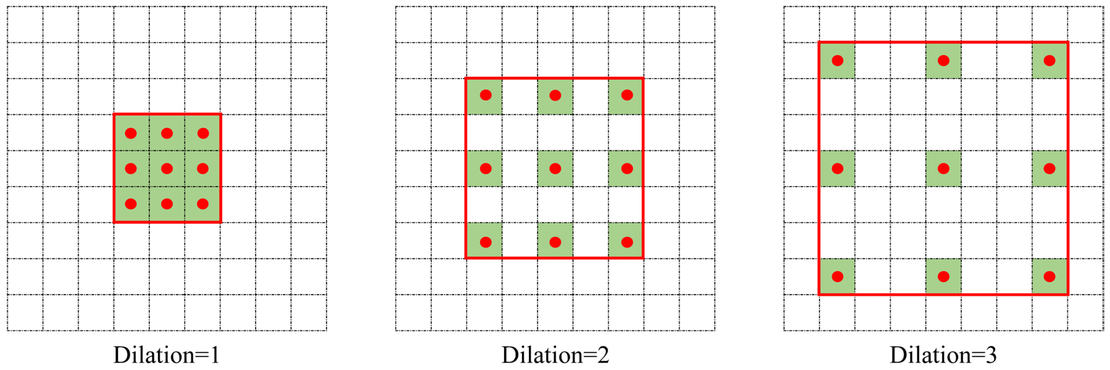
We illustrate the operation of dilated convolution with the example shown in Figure 2. The difference between dilation convolution and conventional convolution is the addition of a hyperparameter termed the dilation rate to the convolution kernel. The size of this controls the number of gaps between sample points in the convolution kernel. In Figure 2, the three images from left to right have dilation rates of 1, 2, and 3, respectively. The comparable convolution kernel size is indicated by the red box area, and the convolution kernel placement is indicated by the red dot. To achieve spacing, a value of 0 is typically entered in the red box blank position. The receptive field remains constant and is the same as the standard convolution when the dilation rate is 1 and the convolution kernel size is 3 × 3 (Figure 2). When the dilation rate is 2, the convolution kernel inserts a row of empty pixels between two nearby locations in the horizontal and vertical directions. This is equivalent to a receptive field with a size of 5 × 5, as in conventional convolution. The receptive field corresponds to a size of 7 × 7 in a typical convolution when the dilation rate is 3. Dilated convolution may successfully capture features at various levels and information at various sizes by expanding the receptive field without growing the convolution kernel by raising the dilation rate. This optimisation maintains computing efficiency while enhancing the model capacity to sense various scales.
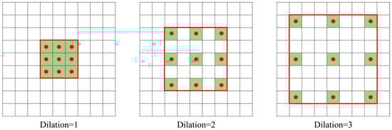
Figure 2.
Working principle of 2D dilated convolution.
The equivalent convolution kernel size and the receptive field size in dilated convolution are represented in Equations (1) and (2), respectively:
where L denotes the equivalent convolution kernel size, l is the size of the original convolution kernel, and the rate is the rate of dilation. Rm+1 is the dilated convolutional layer’s m + 1st receptive field size, and Si denotes the step size of layer i.
When using three or more successive dilated convolutional layers, the design of the dilation rate is especially important. The gridding effect, which is a loss of detailed information and incoherence amongst feature information, can come from improper dilation rate selection and underusing all the data within the corresponding receptive field. Therefore, maintaining detail integrity and feature coherence depends on selecting an appropriate dilation rate. To address the aforementioned issue, hybrid dilated convolution (HDC) [53] is a useful technique. To guarantee optimal performance, HDC uses a sawtooth structure when selecting the expansion factor. The HDC dilation rate size must be designed according to Equation (3)’s specifications.
where di is the Layer I dilation rate. Making Mi ≤ K, where K is the convolution kernel size, is the aim. For instance, the requirement is found to be satisfied for = 2 < K when K = 3 and the dilation rates of the three dilated convolutional layers are d = [1,2,5]. Consequently, in this model, the dilation rates of the dilated convolutional layers in the two branches were set to 1, 2, and 5.
2.2.2. Dilated Spectral–Spatial Feature Extraction
A high spectral index HSI has several spectral bands, and each pixel has rich spectral information. To address the issues of difficulty in feature extraction, redundancy in feature representation, and correlation across categories for HSI data, this model uses a two-branch feature extraction structure. Given that spectral and spatial information are extracted separately in the two branches, they can complementarily represent different aspects of the image. This improves the diversity and differentiation of the features and, thus, improves the classification performance.
To extract shallow spatial features, we used one standard 2D convolutional layer and three consecutive 2D dilated convolutional layers in the spatial branch. Similar to this, we used three successive 1D dilated convolutional layers in the spectral branch and a regular 1D convolutional layer to extract the shallow spectrum characteristics. The space branch operation is next described in detail as an example. A conventional convolutional layer was applied to the patches taken from the HSI to learn low-level edge and texture features that offer rudimentary shape and structural information to gather global information. The resulting feature maps were then input into three successive dilated convolutional layers with dilation rates of 1, 2, and 5. A hierarchical feature learning module was created as a result of this process, which gradually improved the abstraction level and receptive field of feature extraction. We set both branch convolution kernel sizes to 3. The model may retain symmetry when processing images while considering the precise capture of spatial position information and contextual information since this guarantees that the convolution operation has the same receptive field size in each direction. Behind each of the basic convolutional and dilation convolutional layers, we added a batch normalisation layer and an ReLU activation function to increase the network’s nonlinear capacity and to speed up convergence and model generalisation. We performed a splicing operation on the feature maps produced by Layers 1–4 of each branch, drawing inspiration from the ResNet model. represents the spatially spliced feature map and represents the spectrally spliced feature map, and the feature map produced by the two branches is denoted by Equation (4):
where b ∈ {spa, spec} and L ∈ {1,2,3,4}. represents the patch obtained from the HSI. represents the output feature map of the b branch at the L-1 layer. denotes the size of the convolutional kernel, where for two-dimensional convolution and for one-dimensional convolution. ‘’ represents the convolution operation. represents the bias term, and ‘’ denotes the activation function.
Next, we merge and to fuse information from different branches to obtain a richer and integrated feature representation. This fusion enhances the expressiveness and feature diversity of the model. The fusion feature map can be expressed as follows:
where ‘’ denotes merging. The image details, local structure, and global semantic information captured by each convolutional operation are preserved in the fused feature map. This substantially improves the classifier’s ability to perceive and classify feature information at different scales.
2.3. Deep Feature Fusion Backbone
Given that CNNs use a local perceptual field to analyse pictures, each neuron in the network can only perceive a small fraction of the input image. However, when processing HSIs, long-range dependencies need to be recorded because HSI data are strongly connected both geographically and spectrally. In HSIs, a pixel’s class could be connected to its far-off neighbours. In contrast, the transformer plays a significant role in HSI classification tasks given its capacity to handle global contextual information. This enables it to acquire global information about the input image. The transformer was then used as a feature extraction unit in the model presented in this study to extract deep fusion information.
2.3.1. Gaussian Weighted Pixel Embedding
The embedding layer of the Vision Transformer (VIT) model is responsible for converting the incoming picture data into a vector representation that the model can process. The input image is divided by the VIT model into several image blocks, or patches, each of which represents a specific local area of the image. As a result of the embedding layer, each image block is subjected to a linear transformation (often a fully linked layer) to produce a vector representation. However, because this method only considers local parts of the image, the image block representation it produces may make it difficult to model global structures and relationships, especially when working with HSI data that have a lot of context dependencies. The expressive capability of the model may be constrained by the inability of linear transformations employed in embedding, such as fully linked layers, to capture non-linear picture properties and relationships. Given these issues, we suggest an optimisation technique that substitutes pixels for patches in the embedding layer and adds Gaussian weight features. A more detailed description of the details and structure of the image is provided by pixel embedding, which also preserves positional and global information. Pixel embedding collects information about each pixel in an image and maps it separately to a unique vector representation. The capacity to model the overall HSI context is improved by the addition of Gaussian weight features. This allowed us to partially capture the non-linear features and relationships in the image and focus the model more on its main regions and key features.
The GWPE block is shown in Figure 3, and the input to its block is the null-spectrum fusion feature map . and represent Gaussian weight matrices, respectively. denotes the outcome of the features through the embedding layer. This is expressed as shown in the following equation:
Here, denotes the dot product. Mapping to the semantic group SG is conducted by pointwise multiplication of with . Then, the SG is transposed and the softmax function is used to make the transposed SG focus more on important semantic features and suppress unimportant information. SG and are then multiplied with the result after the product to obtain the output feature of the embedding layer.
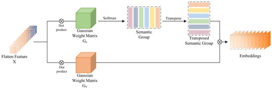

Figure 3.
Visualisation process of the GWPE block.
Figure 3.
Visualisation process of the GWPE block.
2.3.2. Transformer Encoder Block
The MHSA [54] and the feedforward neural network (MLP) layer make up this module, as shown in Figure 1. By creating correlations between input embedding sequences and offering a context-sensitive representation for each vector, the job of the MHSA is to capture global dependencies. Meanwhile, the MLP functions as a local mapping function that aids in the sequence acquisition of regional patterns and contextual data.
The pixel vector features of the input are mapped into distinct vector subspaces named Q (query), K (key), and V (value) by the MHSA to capture feature relationships in various subspaces. A linear transformation is then used to reduce the dimensionality and keep the useful information by concatenating the outputs of several attention heads and projecting them onto the output space. Equation (8) demonstrates how to calculate the similarity between the query and the key:
where the result obtained by dot-multiplying Q with reflects the similarity between these two vectors. To obtain the normalised attention weights, we applied the softmax function to transform the similarity matrix into an attention-weight matrix. The resulting attention-weight matrix is dot-multiplied with the value vector V to obtain the attention value of the MHSA.
The MLP layer conducts nonlinear transformation of attention values and feature extraction in the transformer, transforming the input into a more expressive feature representation. The MLP layer processes the attention values through a combination of multiple linear transformations and nonlinear activation functions. To add more feature dimensions and capture more information, the attention values are first mapped to a higher dimensional space via a first linear transformation. To extract the most valuable characteristics, the expanded feature space is then compressed and reassembled using a second linear transformation. The nonlinear activation function gives the MLP layer nonlinear characteristics, reducing the impact of noise and unimportant data while emphasising and reiterating characteristics pertinent to the modelling objective. Equation (9) can be used to express the MLP layer output:
where and and and are the weights and biases of the two linear transformations, respectively, and ‘’ is the nonlinear activation function. To mitigate covariate bias and provide a relatively stable gradient signal, a layer normalisation (LN) layer was introduced before the MHSA and MLP layers.
3. Experiment and Analysis
3.1. Data Description
This section introduces the five hyperspectral datasets that were used, and Figure 4, Figure 5, Figure 6, Figure 7 and Figure 8 display the raw HSIs and ground truth labelled images of these datasets.
(1) Matiwan Village (MV) dataset: An aerial HSI taken in the Chinese province of Hebei in the village of Matiwan, Xiong’an New Area, Baoding City. With a spectral resolution of 2.1 nm and a range of 400–1000 nm, the dataset consists of 256 bands. The image has a spatial resolution of 0.5 m and 3750 × 1580 image components. Following fieldwork, 18 different varieties of cash crops were chosen as examples for outlining.

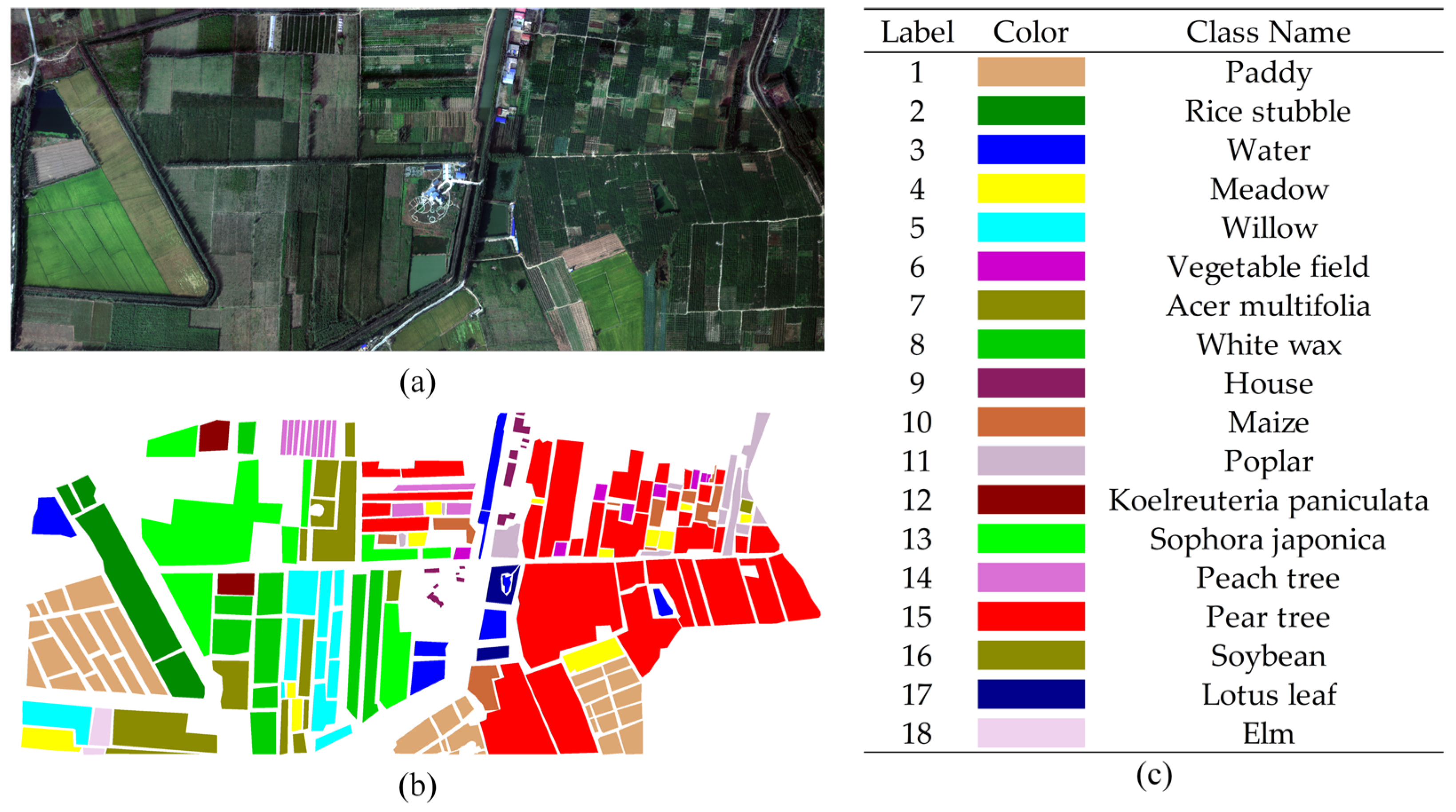
Figure 4.
Original HSI and ground truth labels are included in the MV dataset. (a) Original his, (b) ground truth map, and (c) object names and their corresponding colours.
Figure 4.
Original HSI and ground truth labels are included in the MV dataset. (a) Original his, (b) ground truth map, and (c) object names and their corresponding colours.
(2) WHU-LongKou dataset: This dataset consists of a hyperspectral unmanned aerial vehicle image that was taken in Longkou Town, Hubei Province, China, on 17 July 2018. There were no clouds or rain clouds in the sky during data collection. The dataset has a spatial resolution of approximately 0.463 m and a spatial dimension of 400 × 550 pixels. There are 270 bands in a spectral range of 400–1000 nm. Agriculture constitutes most of the research region and six of the nine elements that were defined are related to agriculture.
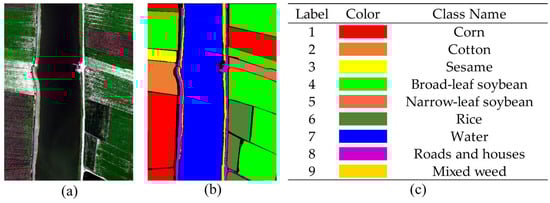
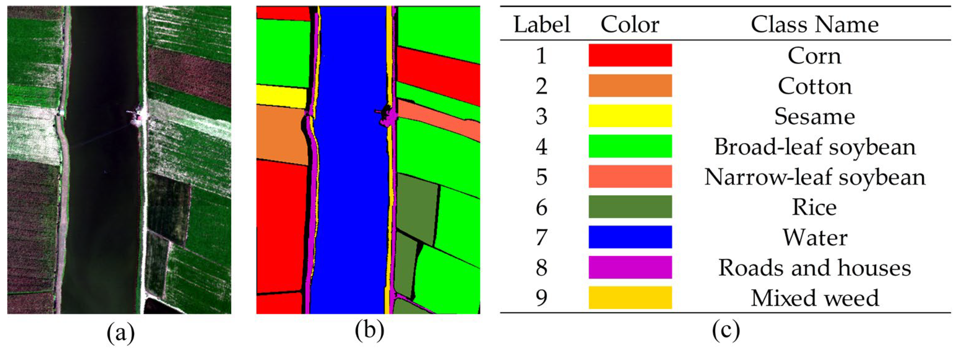
Figure 5.
Original HSI and ground truth labels are included in the WHU-LongKou dataset. (a) Original his, (b) ground truth map, and (c) object names and their corresponding colours.
Figure 5.
Original HSI and ground truth labels are included in the WHU-LongKou dataset. (a) Original his, (b) ground truth map, and (c) object names and their corresponding colours.
(3) WHU-HongHu dataset: This dataset was collected on 20 November 2017 in Honghu City, Hubei Province, China. During the collection process, the UAV data were obscured by a small amount of cloud cover. The dataset has a spatial extent of 940 × 475 pixels, a spatial resolution of 0.043 m, and contains a total of 270 bands. The dataset mainly covers a wide range of complex crop types, and has a high degree of similarity between specific feature classes, such as Chinese cabbage/cabbage and Brassica chinensis/small Brassica chinensis. In total, 22 feature types were outlined.
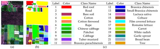
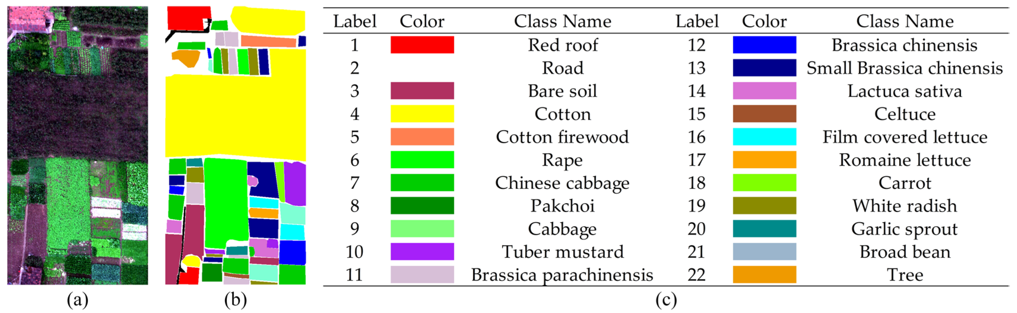
Figure 6.
Original HSI and ground truth labels are included in the WHU-HongHu dataset. (a) Original his, (b) ground truth map, and (c) object names and their corresponding colours.
Figure 6.
Original HSI and ground truth labels are included in the WHU-HongHu dataset. (a) Original his, (b) ground truth map, and (c) object names and their corresponding colours.
(4) Houston dataset: This dataset was provided by the GRSS Data Fusion Contest 2013, and its scope was the University of Houston and its neighbouring cities. The dataset has a spatial extent of 1905 × 349 with a spatial resolution of 2.5 m and a total of 144 bands. The dataset contains 15 different feature classes such as roofs, streets, gravelled roads, grass, trees, water, and shadows.
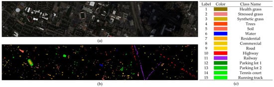
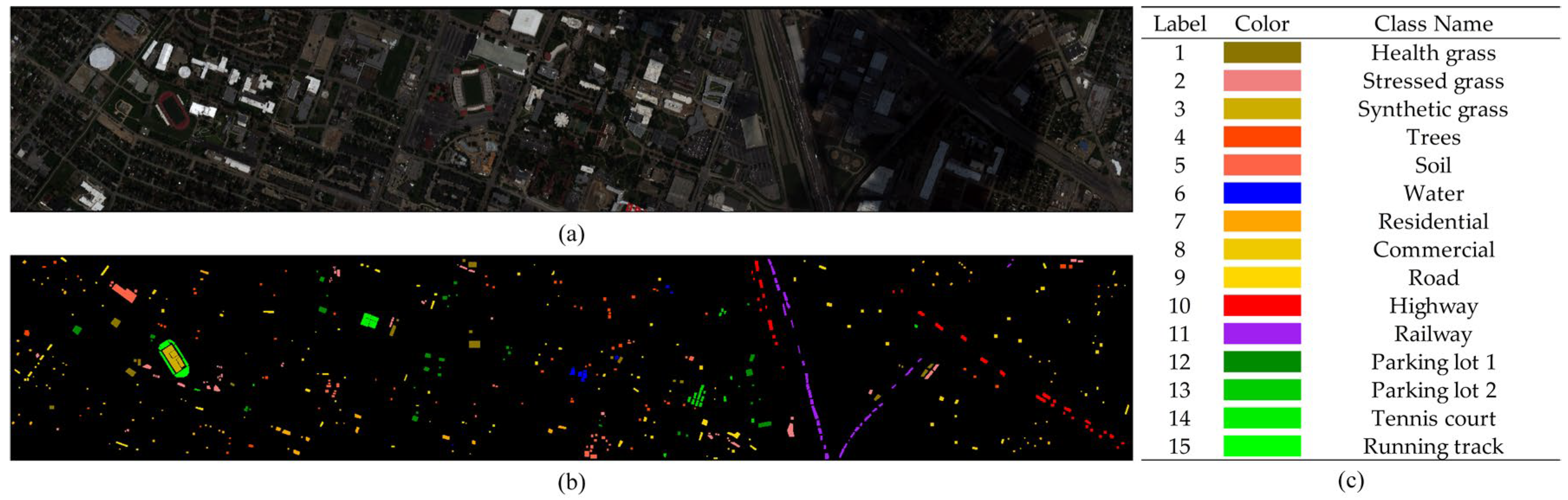
Figure 7.
Original HSI and ground truth labels are included in the Houston dataset. (a) Original his, (b) ground truth map, and (c) object names and their corresponding colours.
Figure 7.
Original HSI and ground truth labels are included in the Houston dataset. (a) Original his, (b) ground truth map, and (c) object names and their corresponding colours.
(5) Pavia Centre (PC) dataset: The northern Italian city of Pavia was the collection point for the PC dataset. The dataset has 102 bands with an image size of 1096 by 715 pixels, spanning the spectral range from 380 nm to 1050 nm. Nine distinct feature classes, including roads, trees, grass, water, and buildings, are present in the dataset.
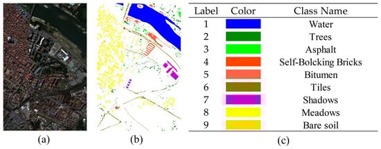
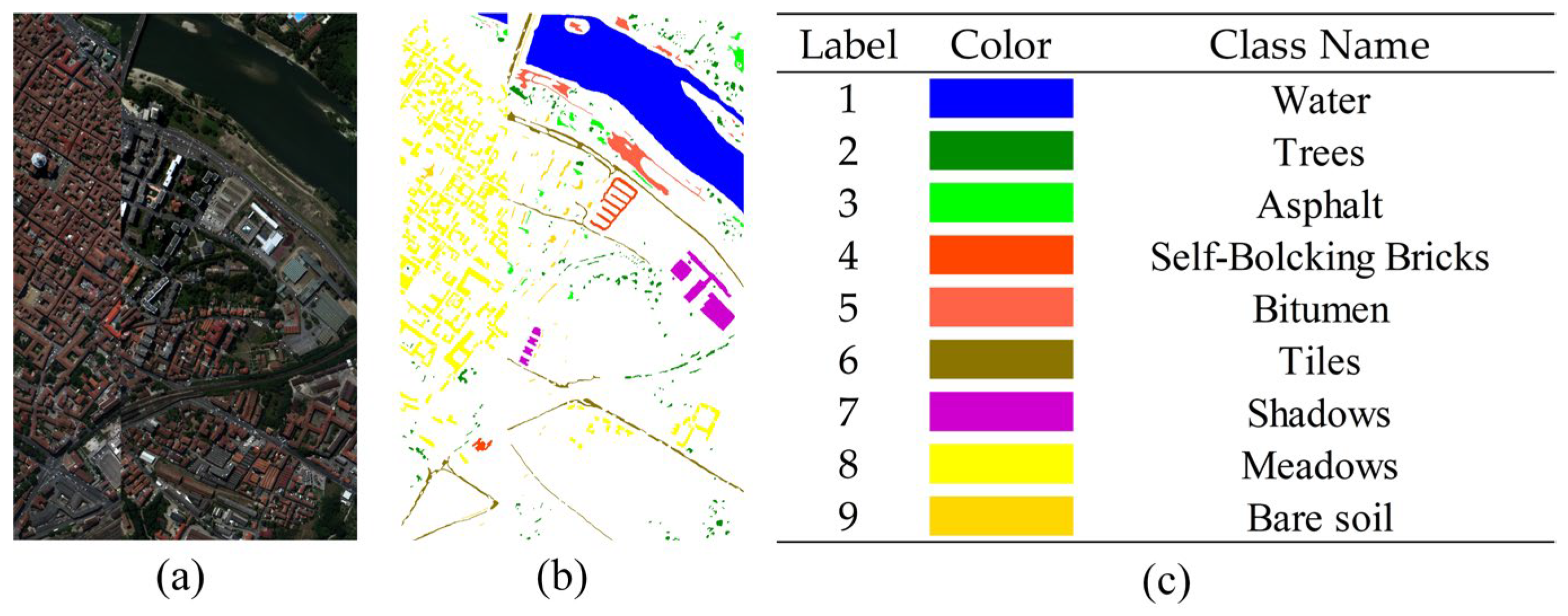
Figure 8.
Original HSI and ground truth labels are included in the PC dataset. (a) Original his, (b) ground truth map, and (c) object names and their corresponding colours.
Figure 8.
Original HSI and ground truth labels are included in the PC dataset. (a) Original his, (b) ground truth map, and (c) object names and their corresponding colours.
3.2. Experimental Setup
(1) Configuration of the workstations: To maintain equity, we conducted the trials using workstations outfitted with Intel(R) Xeon(R) Gold 5218R CPUs, NVIDIA GeForce RTX 3080 GPUs, and 128 GB of RAM, running Windows 10. Using the PyTorch deep learning framework, all the models underwent training. We implemented an early terminating training technique and limited the number of training epochs to 300. This indicated that we would terminate training and store the best model if the loss function stopped decreasing, that is, approached saturation, for 30 consecutive epochs. The early halting method speeds up training while assisting in preventing the overfitting of the model. The experiment results are more reliable because we repeated each experiment ten times and used the mean treatment.
(2) Input settings: We experimented on five datasets, progressively increasing the patch size from 5 × 5 to 15 × 15, to establish the ideal patch size. Considerations were the model computing expense, the accuracy of the experiments, and the capacity of the image to capture rich contextual information and minute features. Ultimately, we decided that the patch input size for this experiment would be 11 × 11.
(3) Sample proportion setting: For the training, validation, and test sets of the five HSI datasets, different sample proportions were used in this experiment. For the MV dataset, 1% of the total data were chosen at random to serve as the training and validation sets, and the other 98% were the test set. From the WHU-LongKou dataset, 99.8% of the labelled data were used for testing, 0.1% for validation, and 0.1% for training. From the WHU-HongHu dataset, 0.5%, 0.5%, and 99% of the samples were chosen for testing, validation, and training, respectively. From the Houston dataset, the percentage of labelled samples used for testing, validation, and training was 90%, 5%, and 5%, respectively. The percentages for the PC dataset were 1%, 1%, and 98%.
(4) Learning rate setting: For this, we experimented with five different learning rates (1E-3, 1E-4, 5E-4, 1E-5, and 5E-5) and tested the model against five datasets. After conducting numerous rounds of trials, we ascertained that 1E-4 represents the ideal learning rate size. The model performance and the outcomes of the experiment were carefully considered before making this decision.
(5) Evaluation Criteria: The overall accuracy (OA), average accuracy (AA), and kappa coefficient were important metrics for evaluating the goodness of the classification results. OA provides an intuitive measure of the overall classification accuracy, AA considers the evaluation in the case of category imbalance, and the kappa coefficient measures the consistency of the model classification results with the randomised classification. Their calculation formulas are as follows:
where represents the overall accuracy of each class, C represents the confusion matrix, and K represents the number of land cover classes in the dataset. Thus, . For any given pixel, represents the number of samples where the jth class is classified as the ith class, represents the number of true labels for the ith class, and represents the number of predicted labels for the ith class. M represents the total number of samples.
3.3. Experimental Results
We compared the proposed method with seven classical and novel deep learning HSI classification models, including 3D-CNN [55], DBDA [40], AB-LSTM [56], HRWN [57], SpectralFormer [58], DFFN [31], and SSFTT [47]. Three convolutional layers and two pooling layers comprise a 3D-CNN. Convolutional layers, spatial attention modules, and channel attention modules are used by DBDA to extract features. Based on a recurrent neural network, the AB-LSTM is a bidirectional long- and short-term memory HSI classification network. An effective hierarchical random walk joint classification network is the hierarchical random walk network. Based on the transformer architecture, SpectralFormer is an HSI classification model that excels at processing high-dimensional, multi-channel data. It extracts features and classifies them using a multilayer perceptron and self-attention mechanism. Recursive learning is used by DFFN, a deep feature fusion network, to streamline the training procedure. High-level semantic characteristics and null-spectrum features are captured using the transformer-based HSI classification model SSFTT.
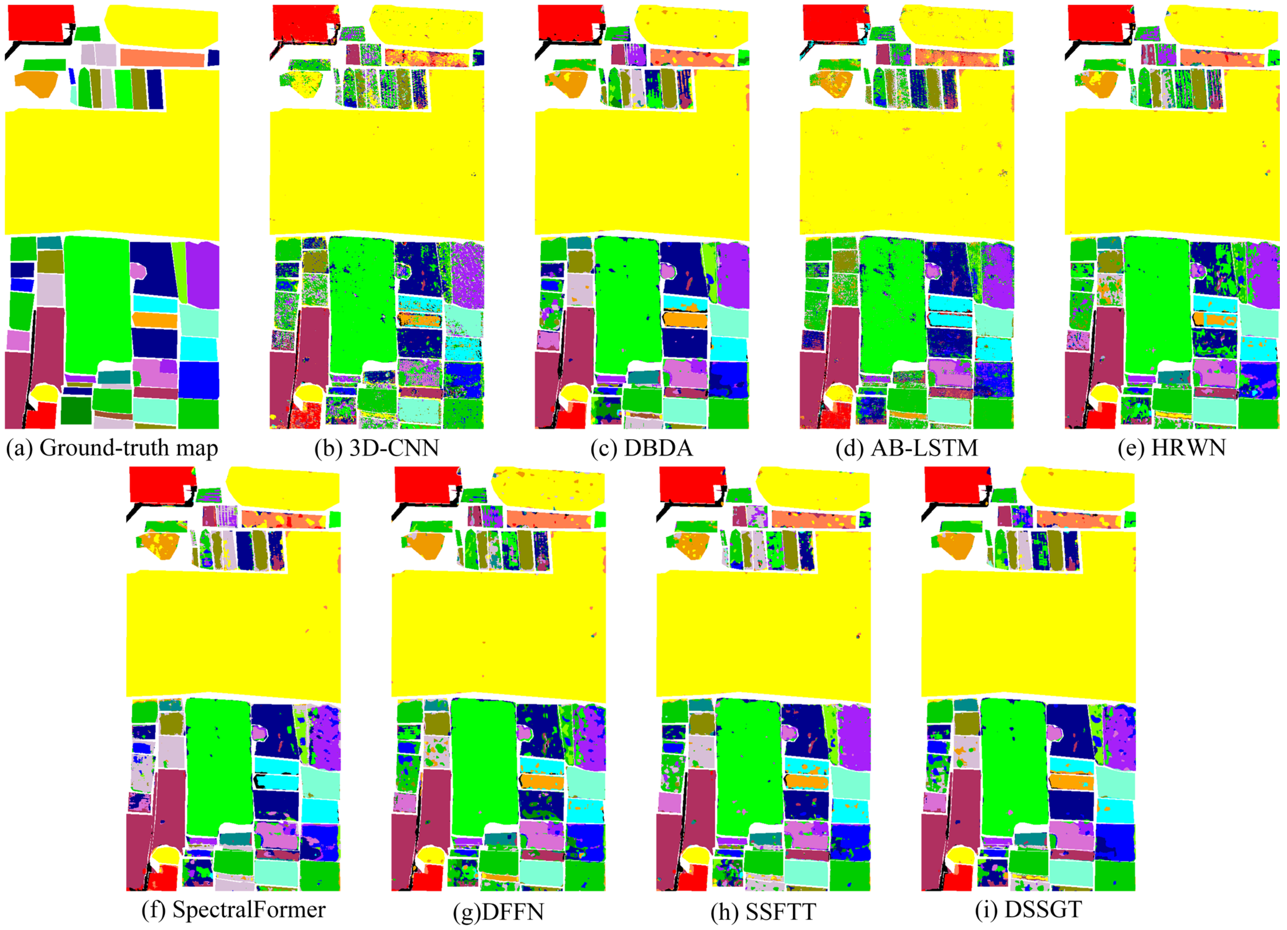
(1) Experimental Results for the MV Dataset: In Table 1 and Figure 9, we show the classification effectiveness of this dataset among eight methods. In Table 1, ‘Train’ represents the number of pixels used for training, while ‘Test’ represents the number of pixels used for testing. The proposed method demonstrated the highest OA, AA, and kappa coefficient on the MV dataset. While DSSGT achieved the highest average precision among the 13 classes, it struggled to accurately classify the ’Maize (label 10)’ and ‘Soybean (label 16)’ land cover types, as observed in Figure 9. Insufficient training samples for these two classes limited the ability of all methods to learn their specific features, resulting in subpar classification performance. However, the GWPE-based transformer module excelled at learning long-range global features from small sample sizes, enabling it to achieve reasonable results even with limited training data. DSSGT boasted an average training time of 7.72 s per epoch, providing a 2.18 s advantage over SSFTT. Although HRWN had the fastest training speed, its classification accuracy fell short. DSSGT tackled this issue by using dilated convolutions as feature extraction units, effectively expanding the receptive field while improving training efficiency. This demonstrated an effective balance between performance and efficiency. The MV dataset primarily consists of land cover types associated with economic crops including maize, soybean, and trees, which share similar spectral characteristics. However, Figure 9 shows that the DSSGT model performed effectively on the MV dataset, yielding the highest similarity between the generated land cover classification map and the ground truth map. This highlights the advantages of DSSGT in capturing subtle spectral differences and spatial contextual information, enabling superior differentiation among these visually similar categories.

Table 1.
Quantitative evaluation was performed on the MV dataset using eight methods (%).
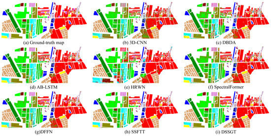
Figure 9.
Classification map derived from eight methods on the MV dataset using 1% of the samples for training. (a) Ground truth map, (b) 3D-CNN (OA = 73.98%), (c) DBDA (OA = 81.57%), (d) AB-LSTM (OA = 87.55%), (e) HRWN (OA = 85.84%), (f) SpectralFormer (OA = 83.53%), (g) DFFN (OA = 89.40%), (h) SSFTT (OA = 93.19%), (i) DSSGT (OA = 95.22%).
(2) Experimental Results for the WHU-LongKou Dataset: Table 2 and Figure 10 contain an accuracy evaluation table and classification effect graphs for this dataset. We only chose 0.1% of the labelled samples as the training set and there were five categories in this training set with less than 10 pixels of training samples. The DSSGT method demonstrated the highest OA of 91.96%, while the DFFN method achieved the highest kappa coefficient (96.51%). All methods exhibited relatively low AA, which suggests a potential impact of data imbalance. The significant disparity in the number of training and testing samples may have adversely affected the performance of the classifiers. To mitigate this issue, the GWPE approach introduced a Gaussian weighted matrix, assigning higher weights to minority classes to give them more attention. Consequently, the DSSGT method achieved the highest AA (66.55%). Figure 10 shows that all methods incorrectly classified ‘Sesame (Label 3)’ as ‘Broad-leaf soybean (Label 4)’. This misclassification can be attributed to the high similarity between these two classes in terms of spectral features, making them challenging to differentiate. However, our proposed method excelled in distinguishing between these two categories by simultaneously extracting spectral, spatial, and texture features from the input data.
Table 2.
Quantitative evaluation was performed on the WHU-LongKou dataset using eight methods (%).
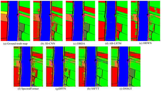
Figure 10.
Classification map derived from eight methods on the WHU-LongKou dataset using 0.1% of the samples for training. (a) Ground truth map, (b) 3DCNN (OA = 82.64%), (c) DBDA (OA = 89.99%), (d) AB-LSTM (OA = 75.32%), (e) HRWN (OA = 81.51%), (f) SpectralFormer (OA = 82.44%), (g) DFFN (OA = 82.77%), (h) SSFTT (OA = 80.55%), (i) DSSGT (OA = 91.96%).
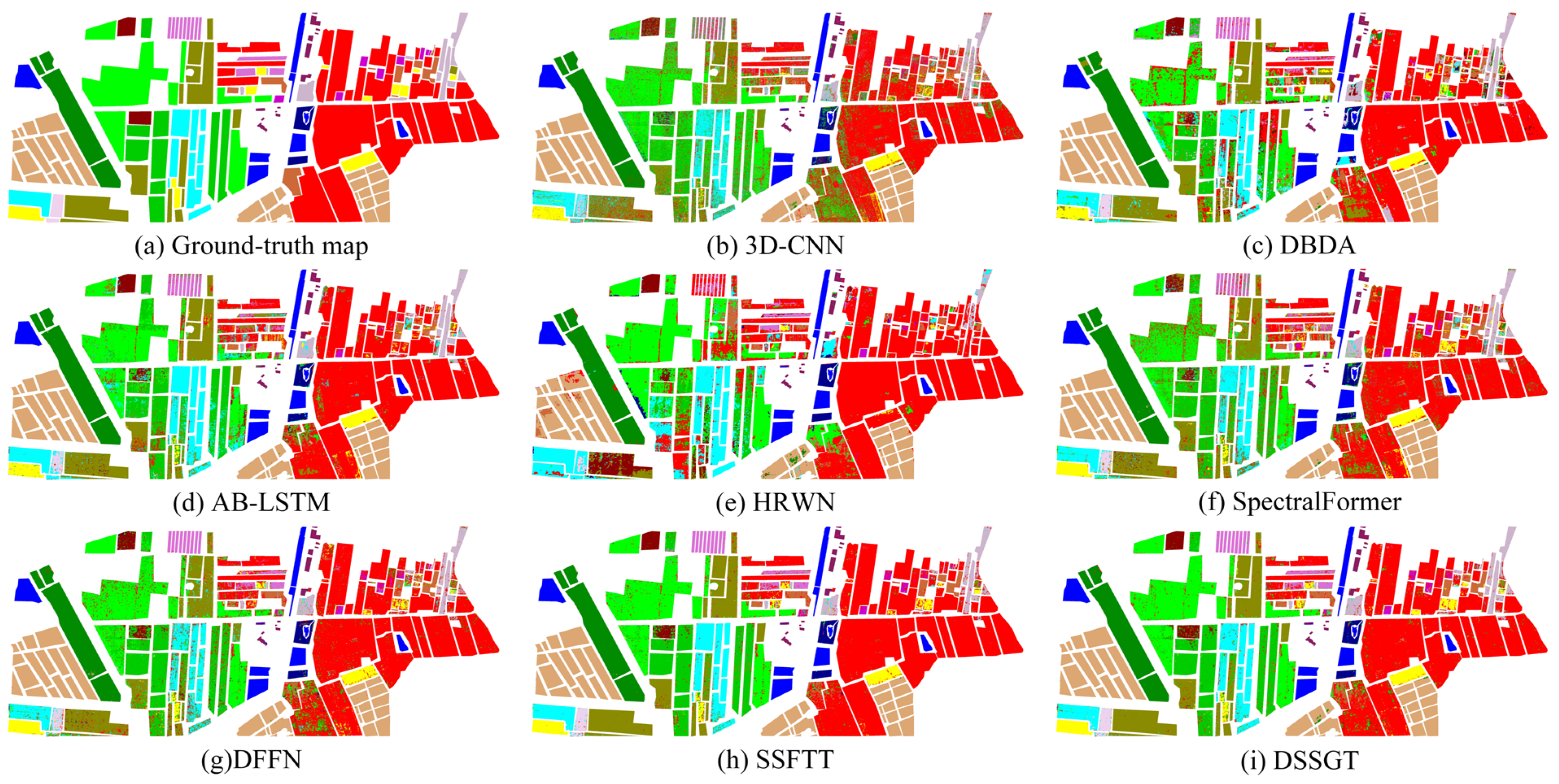
(3) Experimental results for the WHU-HongHu Dataset: Table 3 and Figure 11 illustrate the quantitative evaluation results of the WHU-HongHu dataset. DBDA and SSFTT achieved accuracy results on par with DSSGT, indicating their effective use of spatial–spectral attention mechanisms. By leveraging these mechanisms, they could more effectively capture the interdependencies and contextual information among land cover categories. This enhanced capability allowed the models to accurately discern the spatial distribution patterns of land features, thereby improving the overall classification accuracy. However, while DSSGT excelled in achieving the highest classification accuracy in 11 out of the 22 land cover classes, it accounted for only half of the total classes. This discrepancy may be attributed to the greater similarity among the remaining 11 land cover classes, posing challenges for the classifier to accurately differentiate them. Consequently, future model optimisation efforts should focus on using more refined and sophisticated feature extraction techniques and classifier designs to effectively tackle classes with similar features.
Table 3.
Quantitative evaluation was performed on the WHU-HongHu dataset using eight methods (%).
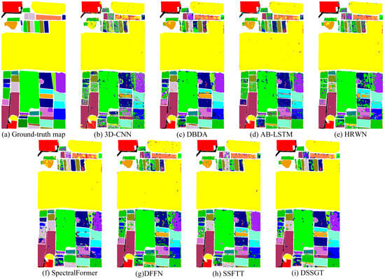
Figure 11.
Classification map derived from eight methods on the WHU-HongHu dataset using 0.5% of the samples for training. (a) Ground truth map, (b) 3DCNN (OA = 83.85%), (c) DBDA (OA = 90.42%), (d) AB-LSTM (OA = 81.96%), (e) HRWN (OA = 86.15%), (f) SpectralFormer (OA = 87.41%), (g) DFFN (OA = 87.63%), (h) SSFTT (OA = 90.28%), (i) DSSGT (OA = 92.64%).
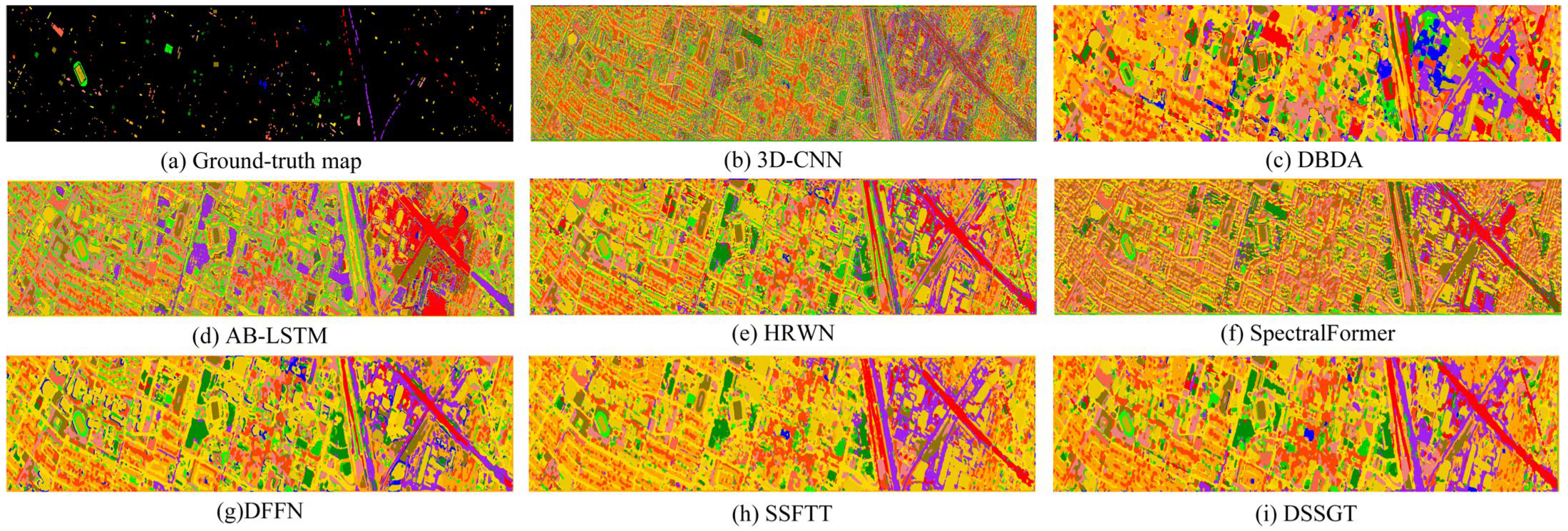
(4) Experimental Results for the Houston Dataset: Figure 12 shows the corresponding feature classification maps, while Table 4 displays the classification outcomes for DSSGT and the other seven classifiers. The classification model appears to have a high level of accuracy overall and across categories and a high level of consistency with the random selection. This is because DSSGT produced the best classification results and the three evaluation factors were relatively close. Given the limited training samples and the variety of data sources, the current dataset DBDA representation is relatively weak. This made it difficult for the conventional two-channel attentional mechanism to effectively capture useful characteristics. Meanwhile, SSFTT and DSSGT based on MHSA can better understand the long-distance connections between features, which enhances the classification outcomes. The classification maps generated using 3D-CNN exhibit numerous isolated noise points and discontinuous pixels, indicating a considerable issue with salt-and-pepper noise. This could be attributed to the limited robustness of 3D-CNN in handling noise and variations in details during land cover classification. Meanwhile, DBDA struggles to differentiate subtle variations between different species, incorrectly categorising large patches as the same category and disregarding inter-species differences. In contrast, the classification maps produced by DFFN, SSFTT, and DSSGT show significant improvements. These models demonstrated enhanced accuracy in identifying subtle variations and differences between species, effectively eliminating the salt-and-pepper noise phenomenon, and improving image quality.
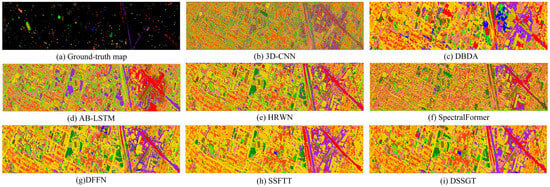
Figure 12.
Classification map derived from eight methods on the Houston dataset using 5% of the samples for training. (a) Ground truth map, (b) 3D-CNN (OA = 62.23%), (c) DBDA (OA = 53.96%), (d) AB-LSTM (OA = 61.31%), (e) HRWN (OA = 92.21%), (f) SpectralFormer (OA = 67.94%), (g) DFFN (OA = 91.17%), (h) SSFTT (OA = 95.57%), (i) DSSGT (OA = 96.72%).
Table 4.
Quantitative evaluation was performed on the Houston dataset using eight methods (%).
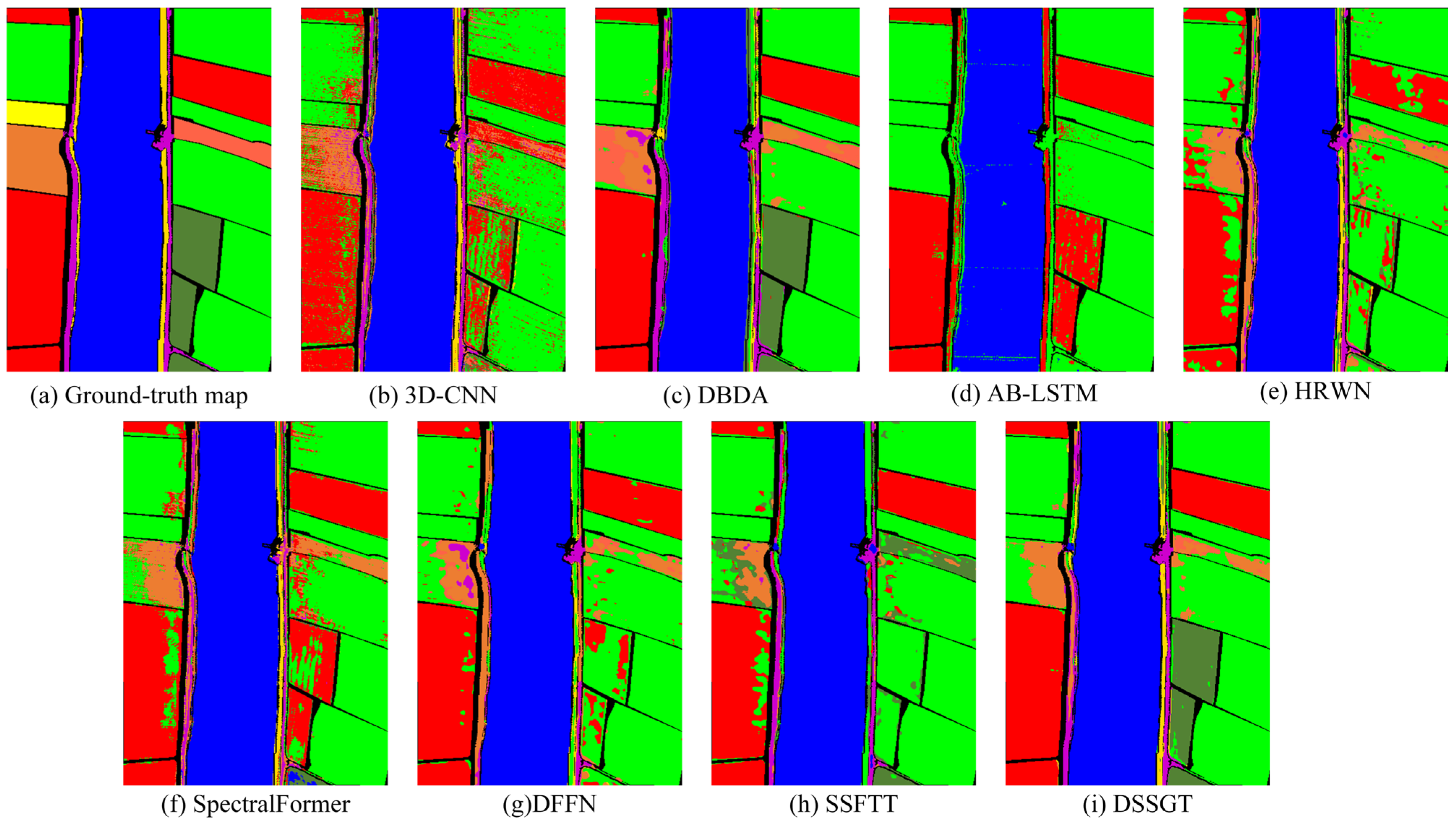
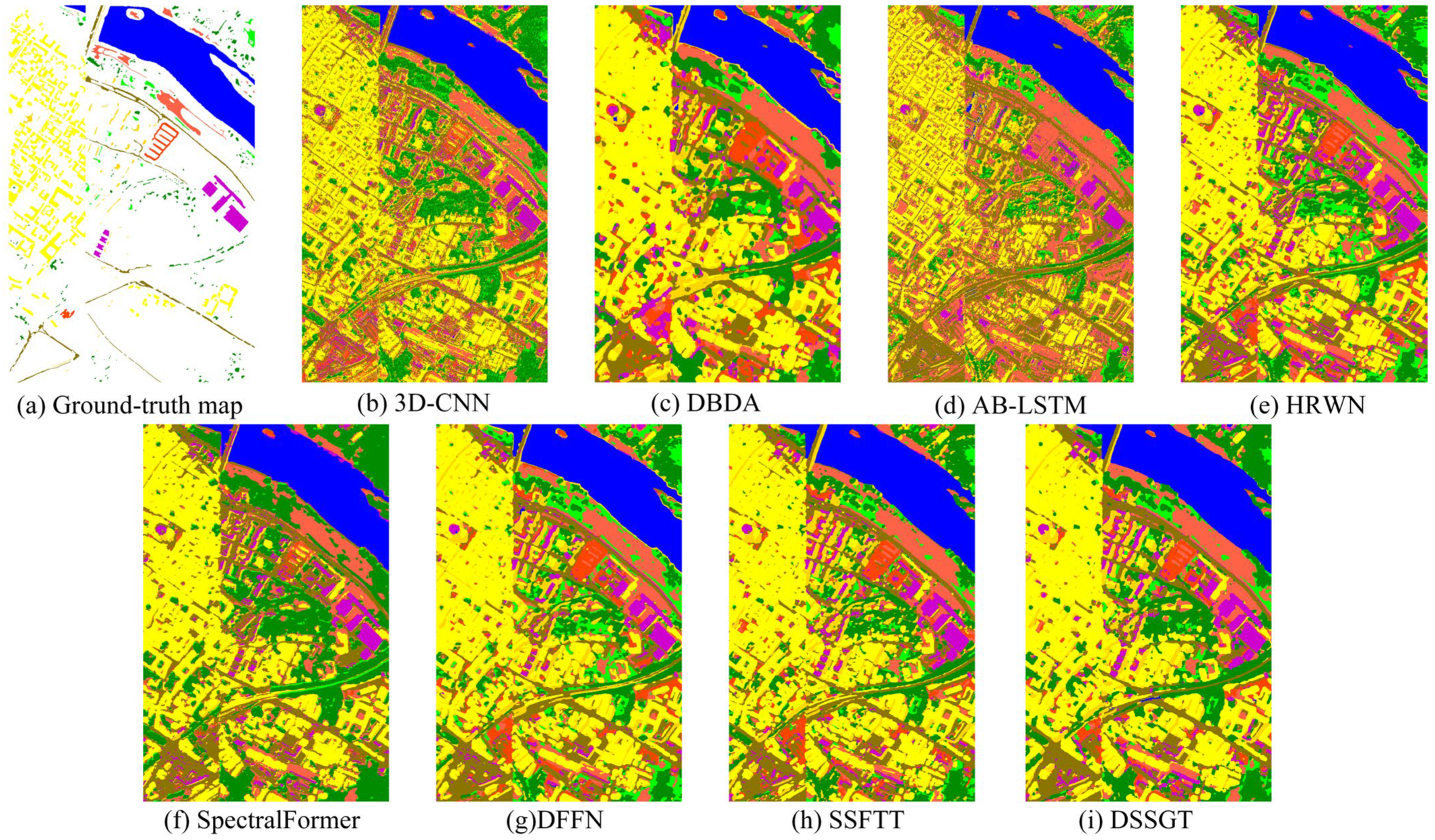
(5) Experimental Results for the PC Dataset: The findings of the quantitative evaluation metrics and classification plots for the PC dataset are shown in Table 5 and Figure 13. In this dataset, DSSGT outperformed other methods in terms of evaluation metrics such as OA, AA, and the kappa coefficient. This highlights its effectiveness in capturing complex spatial relationships between land cover categories. This indicates that DSSGT exhibits stronger capabilities in modelling dependencies and contextual information among different land features, resulting in more accurate and consistent classification results. The observed discontinuities and patchy patterns in the classification maps generated by 3D-CNN and AB-LSTM raise concerns about their ability to capture fine-grained details and handle spatial variations. This can lead to misclassifications and inconsistencies in land cover recognition. In contrast, the classification maps generated by DSSGT are smooth and accurate, demonstrating its ability to effectively eliminate patchy structures and produce visually coherent results. This is attributed to the attention mechanisms and the model’s ability to capture long-range dependencies, enabling it to better capture spatial context and generate more refined classification boundaries.
Table 5.
Quantitative evaluation was performed on the PC dataset using eight methods (%).
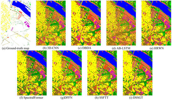
Figure 13.
Classification map derived from eight methods on the PC dataset, using 1% of the samples for training. (a) Ground truth map, (b) 3D-CNN (OA = 93.13%), (c) DBDA (OA = 94.94%), (d) AB-LSTM (OA = 94.69%), (e) HRWN (OA = 98.66%), (f) SpectralFormer (OA = 96.04%), (g) DFFN (OA = 98.50%), (h) SSFTT (OA = 98.99%), and (i) DSSGT (OA = 99.13%).
3.4. Discussion
3.4.1. Ablation Experiments
We performed ablation tests on five datasets to validate the efficacy of the novel component of our suggested technique. The effectiveness of the dilated convolution in comparison to that of the standard convolution was assessed in the first section of the ablation experiments, and the effectiveness of the GWPE block was assessed in the second section. The experimental results are presented in Table 6, where each dataset’s first row represents the usage of standard convolution with GWPE. The second row corresponds to the usage of dilated convolution without GWPE, and the third row represents the usage of dilated convolution with GWPE.
Table 6.
Ablation experiments on five datasets using the proposed model.
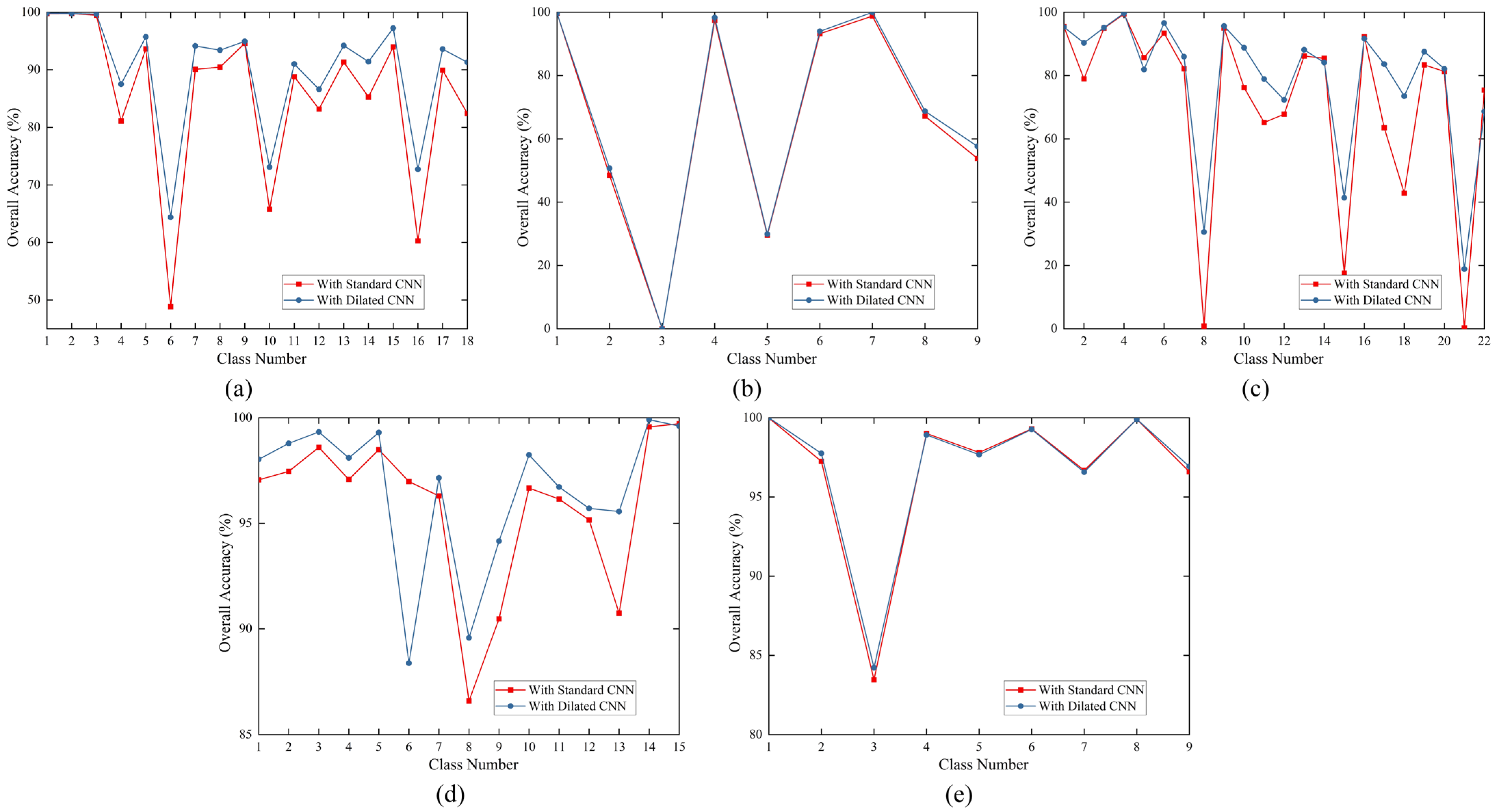
(1) Impact of dilated convolutions: Table 6 shows the results from adjusting the variables using the GWPE scenario, using standard and dilated convolution, respectively, in the first and third rows of each dataset. In all five datasets, utilising dilated convolution resulted in greater OA, AA, and kappa coefficients than doing so with normal convolution. This is because our model’s input patch size was 11. The range of the receptive field included the global data of the input patches when we used three consecutive dilated convolutional layers with dilation rates of one, two, and five. This architecture enhanced the model’s performance on the dataset by enabling it to capture the contextual and general aspects of the input data more effectively. Figure 14 uses standard and dilated convolution for each category to illustrate the effects of DSSGT on five datasets. The graphed results show that the accuracy of feature categorisation is not significantly affected by the type of convolution used, for both the WHU-LongKou and PC datasets. The usage of dilated convolution performs better in several of the poorly categorised feature classes, as shown by the other three datasets. Specific categories that benefited from the use of dilation convolution include ‘vegetable field (Label 6)’ in the MV dataset, ‘Pakchoi (Label 8)’ in the WHU-HongHu dataset, and ‘commercial (Label 8)’ in the Houston dataset. This shows that dilation convolution has an advantage over typical standard convolution in capturing feature categories whose features are concealed or inconspicuous and can do so more effectively.
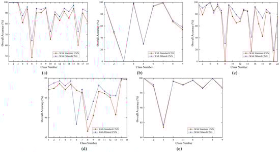
Figure 14.
Impact of DSSGT on the classification results of each class in five datasets using either standard convolution or dilated convolution. (a) MV, (b)WHU-LongKou, (c) WHU-HongHu, (d) Houston, and (e) PC.
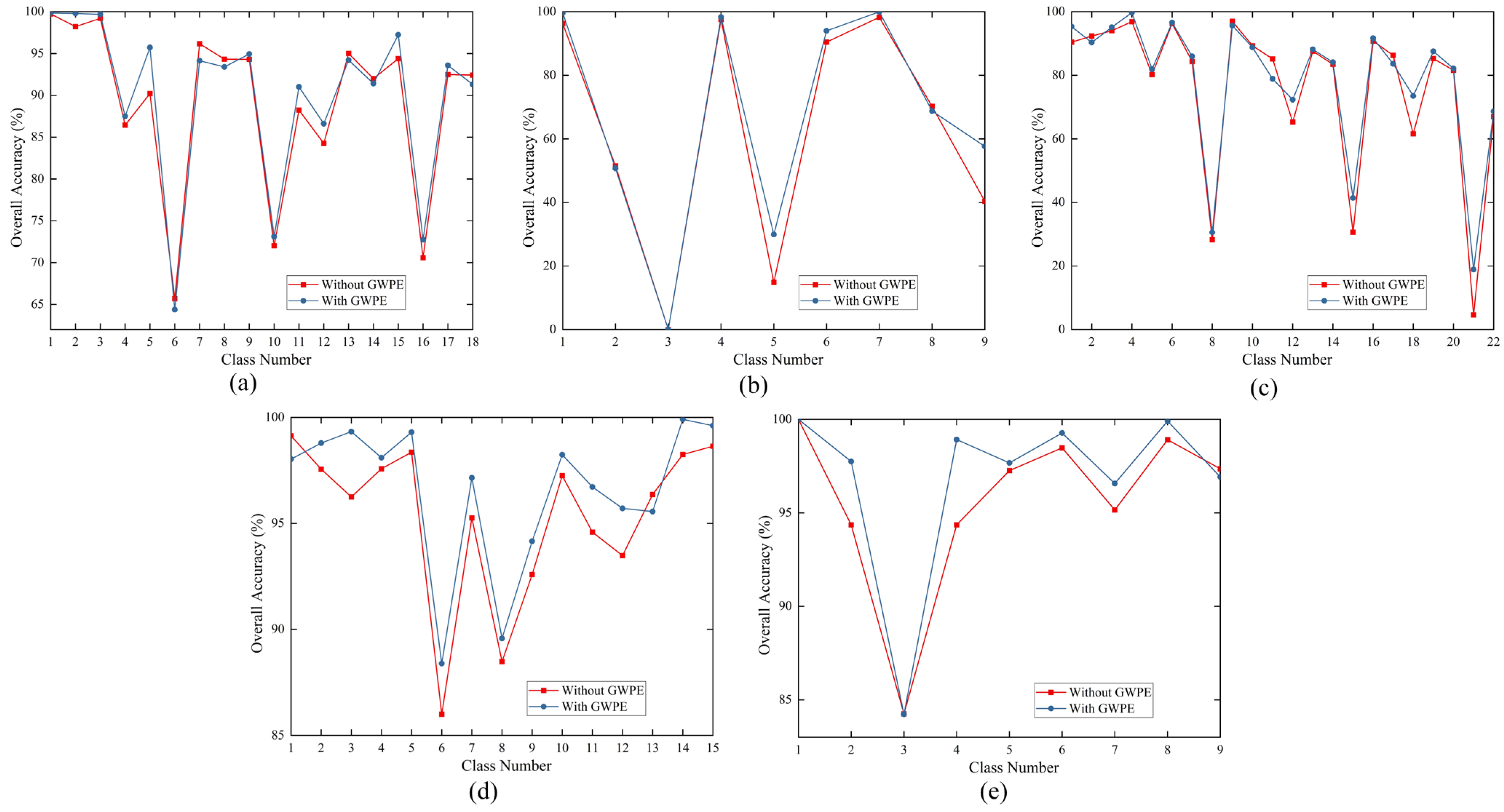
(2) Impact of GWPE: GWPE is the most critical component of the DSSGT module. It enhances the classification performance by introducing Gaussian weights to emphasise important parts of the input features. In Table 6, the second and third rows for each dataset represent the classification results with and without the GWPE module, respectively. Figure 15 shows the influence of GWPE on each category. The framework with GWPE achieved an OA improvement of 3.7% compared to the regular framework on the MV dataset. Similar results were observed with the WHU-LongKou and WHU-HongHu datasets, with an OA increase of approximately 1% in both cases. However, given the already high initial OA values in the Houston and PC datasets, the improvement brought by GWPE is not significant. Nevertheless, the annotations in Figure 15 indicate that GWPE has a positive impact on all land cover classification tasks in the Houston and PC datasets. The introduction of GWPE enables the model to more effectively capture the distinctions between land cover categories and the correlations among features, significantly enhancing the classification accuracy and performance.
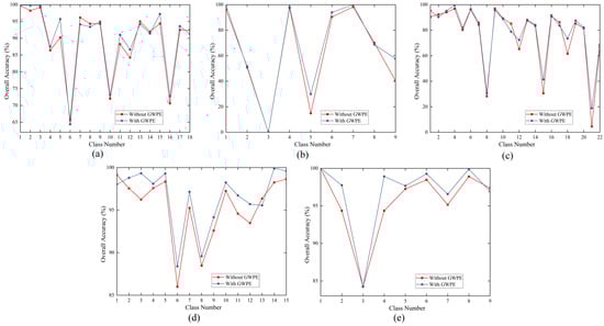
Figure 15.
Impact of applying GWPE in DSSGT on the classification results in each class for five datasets. (a) MV, (b) WHU-LongKou, (c) WHU-HongHu, (d) Houston, and (e) PC.
3.4.2. Robustness Evaluation
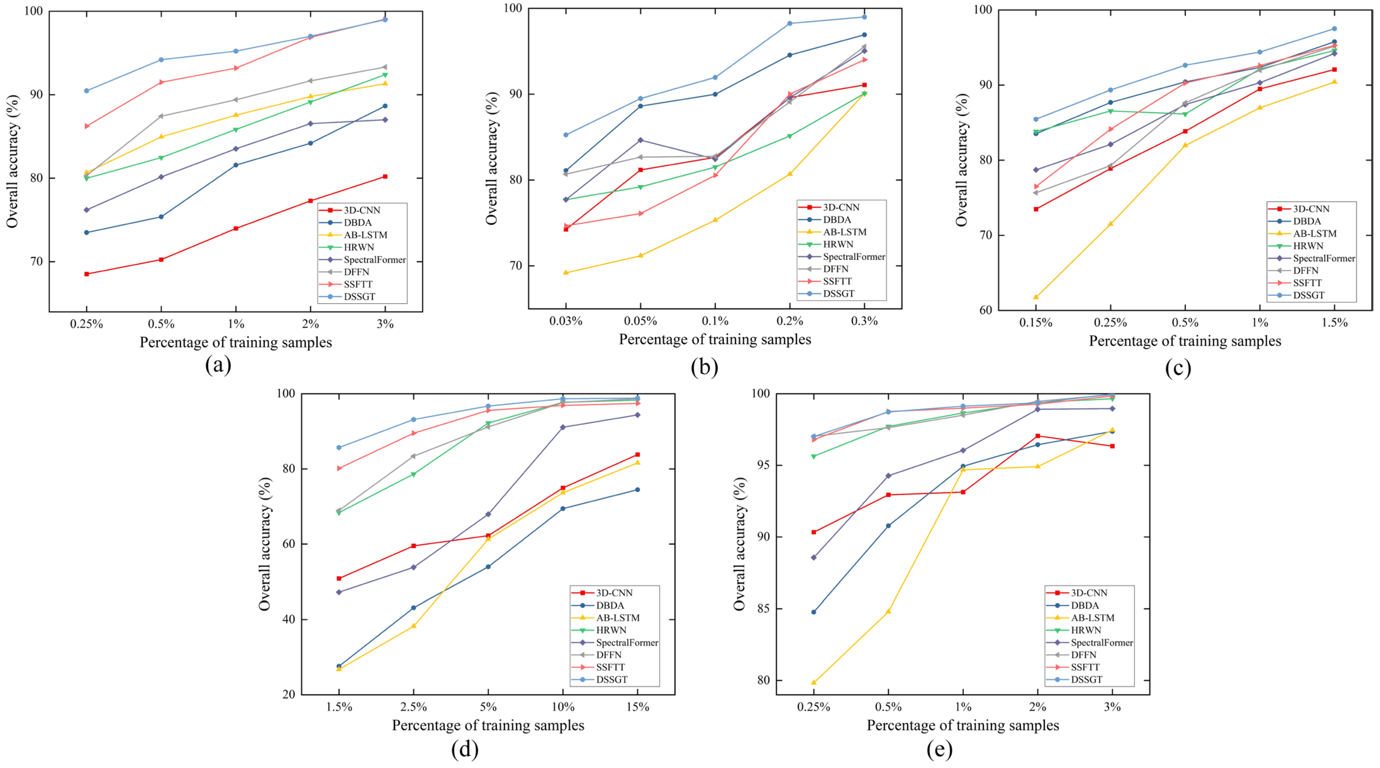
We conducted tests on five datasets to examine the impact of various ratios on the outcomes by reducing or increasing the number of their training samples by two or three times, respectively. This was performed to ensure the stability of the suggested strategy. For instance, we selected the 0.25%, 0.5%, 2%, and 3% labelled samples as the training set for the MV dataset. Figure 16 shows the quantitative results of different classifiers, which demonstrate that DSSGT outperformed the other methods. However, the improvement in DSSGT compared to other methods is not significant for datasets such as WHU-LongKou, Houston, and PC, which have a large proportion of training samples. Meanwhile, when faced with extremely limited sample sizes, the advantage of DSSGT becomes more pronounced. This indicates that the proposed method not only performs well with an ample amount of sample data but also demonstrates superior results in scenarios with limited sample data. In contrast, AB-LSTM performs poorly in small-sample scenarios, emphasising the superiority and stability of DSSGT in addressing data scarcity issues.
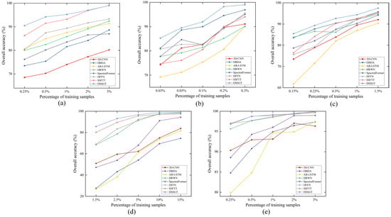
Figure 16.
Comparison of OAs for eight methods under various training ratios. (a) MV, (b) WHU-LongKou, (c) WHU-HongHu, (d) Houston, and (e) PC.
4. Conclusions
In this study, we proposed a novel HSI classification model called DSSGT. Our model incorporates several key components aimed at improving performance and enhancing contextual understanding of the classification task. We introduced a feature extraction module based on dilated convolutions to effectively capture shallow spectral features within input image patches. By stacking multiple dilated convolutional layers with varying dilation rates but the same kernel size, we expanded the receptive field. This design enabled us to capture a wider range of contextual information while preserving local details. Through the progressive stacking of dilated convolutional layers, we gradually extended the feature extraction range, enabling the model to more effectively comprehend the global structure and relationships within the input data. Next, we fed the extracted shallow features from the feature extraction module into the GWPE module, transforming them into pixel-level vector representations. This module combines the features of each pixel with its surrounding pixels in a Gaussian weighted manner, thereby generating more expressive and context-aware pixel-level representations. We then input the obtained pixel-level vector matrix into the transformer encoder blocks to generate deep long-range fused features. By stacking MLP and MHSA layers, we could effectively capture global dependencies within the input data and generate more expressive and discriminative feature representations. We performed global average pooling on the deep long-range fused features to generate a classification probability map. This map provided category probability information for each pixel in the HSI. We conducted comparative experiments on five datasets, comparing DSSGT with seven state-of-the-art methods. The consistent experimental results have demonstrated the substantial advantages of DSSGT across all datasets, validating the effectiveness of our proposed approach.
Author Contributions
Conceptualization, Z.Z. and S.W.; methodology, Z.Z.; software, S.W.; validation, Z.Z., W.Z. and S.W.; formal analysis, Z.Z.; investigation, Z.Z.; resources, S.W.; data curation, S.W.; writing—original draft preparation, Z.Z.; writing—review and editing, Z.Z.; visualization, S.W.; supervision, W.Z.; project administration, S.W.; funding acquisition, W.Z. All authors have read and agreed to the published version of the manuscript.
Funding
This work was co-supported by the National Natural Science Foundation of China (Grant 41672358), the Second Tibetan Plateau Scientific Expedition and Research (2019QZKK0707), and the Basic Science Centre for Tibetan Plateau Earth System (CTPES, Grant 41988101-01).
Data Availability Statement
The MV dataset used in this study is available at http://www.hrs-cas.com/a/share/shujuchanpin/2019/0501/1049.html, accessed on 15 August 2023; the WHU-HongHu and WHU-LongKou dataset used in this study are available at http://rsidea.whu.edu.cn/resource_WHUHi_sharing.htm, accessed on 15 August 2023; the Houston dataset used in this study is available at https://hyperspectral.ee.uh.edu/?page_id=1075, accessed on 15 August 2023; the PC dataset is available from https://www.ehu.eus/ccwintco/index.php/Hyperspectral_Remote_Sensing_Scenes, accessed on 15 August 2023.
Conflicts of Interest
The authors declare no conflicts of interest.
References
- Liu, M.; Zhao, J.; Zheng, J.; Wu, R. Review of Hyperspectral Imaging in Quality and Safety Inspections of Agricultural and Poultry Products. Trans. Chin. Soc. Agric. Mach. 2005, 36, 139–143. [Google Scholar]
- Wu, D.; Sun, D.-W. Advanced applications of hyperspectral imaging technology for food quality and safety analysis and assessment: A review—Part I: Fundamentals. Innov. Food Sci. Emerg. Technol. 2013, 19, 1–14. [Google Scholar] [CrossRef]
- Cui, R.; Yu, H.; Xu, T.; Xing, X.; Cao, X.; Yan, K.; Chen, J. Deep Learning in Medical Hyperspectral Images: A Review. Sensors 2022, 22, 9790. [Google Scholar] [CrossRef]
- Gerdes, N.; Hoff, C.; Hermsdorf, J.; Kaierle, S.; Overmeyer, L. Hyperspectral imaging for prediction of surface roughness in laser powder bed fusion. Int. J. Adv. Manuf. Technol. 2021, 115, 1249–1258. [Google Scholar] [CrossRef]
- Dong, X.; Yan, B.; Gan, F.; Li, N. Progress and prospectives on engineering application of hyperspectral remote sensing for geology and mineral resources. In Proceedings of the Fifth Symposium on Novel Optoelectronic Detection Technology and Application, Xi’an, China, 24–26 October 2018; SPIE: Bellingham, WA, USA, 2019. [Google Scholar]
- Luo, H.; Kan, Y.; Wang, L.; Fang, J.; Dai, S. Hyperspectral remote sensing for crop diseases and pest dectection. Guandong Agric. Sci. 2012, 39, 76–80. [Google Scholar]
- Sun, L.; He, C.; Zheng, Y.; Tang, S. SLRL4D: Joint Restoration of Subspace Low-Rank Learning and Non-Local 4-D Transform Filtering for Hyperspectral Image. Remote Sens. 2020, 12, 2979. [Google Scholar] [CrossRef]
- Wang, R.; Li, H.-C.; Liao, W.; Huang, X.; Philips, W. Centralized Collaborative Sparse Unmixing for Hyperspectral Images. IEEE J. Sel. Top. Appl. Earth Obs. Remote Sens. 2017, 10, 1949–1962. [Google Scholar] [CrossRef]
- Mou, L.; Ghamisi, P.; Zhu, X.X. Deep Recurrent Neural Networks for Hyperspectral Image Classification. IEEE Trans. Geosci. Remote Sens. 2017, 55, 3639–3655. [Google Scholar] [CrossRef]
- Ge, H.; Tang, Y.; Bi, Z.; Zhan, T.; Xu, Y.; Song, A. MMSRC: A Multidirection Multiscale Spectral-Spatial Residual Network for Hyperspectral Multiclass Change Detection. IEEE J. Sel. Top. Appl. Earth Obs. Remote Sens. 2022, 15, 9254–9265. [Google Scholar] [CrossRef]
- Hou, Z.; Li, W.; Li, L.; Tao, R.; Du, Q. Hyperspectral Change Detection Based on Multiple Morphological Profiles. IEEE Trans. Geosci. Remote Sens. 2022, 60, 5507312. [Google Scholar] [CrossRef]
- Chen, H.; Du, X.; Liu, Z.; Cheng, X.; Zhou, Y.; Zhou, B. Target Recognition Algorithm for Fused Hyperspectral Image by Using Combined Spectra. Spectrosc. Lett. 2015, 48, 251–258. [Google Scholar] [CrossRef]
- Haitao, L.I.; Haiyan, G.U.; Bing, Z.; Lianru, G.A.O. Research on Hyperspectral Remote Sensing Image Classification Based on MNF and SVM. Remote Sens. Inf. 2007, 12–15, 25. [Google Scholar]
- Ma, X.; Yan, W.; Bian, H.; Sun, B.; Wang, P. Hyperspectral Remote Sensing Classification Based on SVM with End-member Extraction. In Proceedings of the MIPPR 2013: Remote Sensing Image Processing, Geographic Information Systems, and Other Applications, Wuhan, China, 26–27 October 2013; SPIE: Bellingham, WA, USA, 2013. [Google Scholar]
- Li, Y.; Wang, H.; Lv, X. The Comparison of Several Classification Algorithms and Case Analysis. In Proceedings of the International Conference on Graphic and Image Processing (ICGIP 2012), Singapore, 5–7 October 2012; SPIE: Bellingham, WA, USA, 2013. [Google Scholar]
- Zeng, Y.; Yang, Y.; Zhao, L. Nonparametric classification based on local mean and class statistics. Expert Syst. Appl. 2009, 36, 8443–8448. [Google Scholar] [CrossRef]
- Dalla Mura, M.; Villa, A.; Benediktsson, J.A.; Chanussot, J.; Bruzzone, L. Classification of Hyperspectral Images by Using Extended Morphological Attribute Profiles and Independent Component Analysis. IEEE Geosci. Remote Sens. Lett. 2011, 8, 542–546. [Google Scholar] [CrossRef]
- Su, H.; Sheng, Y.; Du, P.; Chen, C.; Liu, K. Hyperspectral image classification based on volumetric texture and dimensionality reduction. Front. Earth Sci. 2015, 9, 225–236. [Google Scholar] [CrossRef]
- Wang, Z.; Du, B.; Zhang, L.; Zhang, L. Based on Texture Feature and Extend Morphological Profile Fusion for Hyperspectral Image Classification. Acta Photonica Sin. 2014, 43, 0810002. [Google Scholar] [CrossRef]
- Licciardi, G.; Marpu, P.R.; Chanussot, J.; Benediktsson, J.A. Linear Versus Nonlinear PCA for the Classification of Hyperspectral Data Based on the Extended Morphological Profiles. IEEE Geosci. Remote Sens. Lett. 2012, 9, 447–451. [Google Scholar] [CrossRef]
- Ren, Y.; Liao, L.; Maybank, S.J.; Zhang, Y.; Liu, X. Hyperspectral Image Spectral-Spatial Feature Extraction via Tensor Principal Component Analysis. IEEE Geosci. Remote Sens. Lett. 2017, 14, 1431–1435. [Google Scholar] [CrossRef]
- Liu, J. Hyperspectral Remote Sensing Image Terrain Classification Based on Direct LDA. Comput. Sci. 2011, 38, 274–277. [Google Scholar]
- Yang, M.; Fan, Y.; Li, B. Research on dimensionality reduction and classification of hyperspectral images based on LDA and ELM. J. Electron. Meas. Instrum. 2020, 34, 190–196. [Google Scholar]
- Hu, W.; Huang, Y.; Wei, L.; Zhang, F.; Li, H. Deep Convolutional Neural Networks for Hyperspectral Image Classification. J. Sens. 2015, 2015, 258619. [Google Scholar] [CrossRef]
- Yang, X.; Zhang, X.; Ye, Y.; Lau, R.Y.K.; Lu, S.; Li, X.; Huang, X. Synergistic 2D/3D Convolutional Neural Network for Hyperspectral Image Classification. Remote Sens. 2020, 12, 2033. [Google Scholar] [CrossRef]
- Shi, C.; Liao, D.; Zhang, T.; Wang, L. Hyperspectral Image Classification Based on Expansion Convolution Network. IEEE Trans. Geosci. Remote Sens. 2022, 60, 5528316. [Google Scholar] [CrossRef]
- Li, J.; Zhao, X.; Li, Y.; Du, Q.; Xi, B.; Hu, J. Classification of Hyperspectral Imagery Using a New Fully Convolutional Neural Network. IEEE Geosci. Remote Sens. Lett. 2018, 15, 292–296. [Google Scholar] [CrossRef]
- He, N.; Paoletti, M.E.; Mario Haut, J.; Fang, L.; Li, S.; Plaza, A.; Plaza, J. Feature Extraction with Multiscale Covariance Maps for Hyperspectral Image Classification. IEEE Trans. Geosci. Remote Sens. 2019, 57, 755–769. [Google Scholar] [CrossRef]
- Roy, S.K.; Krishna, G.; Dubey, S.R.; Chaudhuri, B.B. HybridSN: Exploring 3-D–2-D CNN Feature Hierarchy for Hyperspectral Image Classification. IEEE Geosci. Remote Sens. Lett. 2020, 17, 277–281. [Google Scholar] [CrossRef]
- He, K.; Zhang, X.; Ren, S.; Sun, J. Deep Residual Learning for Image Recognition. In Proceedings of the 2016 IEEE Conference on Computer Vision and Pattern Recognition (CVPR), Las Vegas, NV, USA, 27–30 June 2016; IEEE: New York, NY, USA, 2016; pp. 770–778. [Google Scholar]
- Song, W.; Li, S.; Fang, L.; Lu, T. Hyperspectral Image Classification with Deep Feature Fusion Network. IEEE Trans. Geosci. Remote Sens. 2018, 56, 3173–3184. [Google Scholar] [CrossRef]
- Feng, F.; Zhang, Y.; Zhang, J.; Liu, B. Small Sample Hyperspectral Image Classification Based on Cascade Fusion of Mixed Spatial-Spectral Features and Second-Order Pooling. Remote Sens. 2022, 14, 505. [Google Scholar] [CrossRef]
- Meng, Z.; Zhao, F.; Liang, M.; Xie, W. Deep Residual Involution Network for Hyperspectral Image Classification. Remote Sens. 2021, 13, 3055. [Google Scholar] [CrossRef]
- Wang, S.; Liu, Z.; Chen, Y.; Hou, C.; Liu, A.; Zhang, Z. Expansion Spectral-Spatial Attention Network for Hyperspectral Image Classification. IEEE J. Sel. Top. Appl. Earth Obs. Remote Sens. 2023, 16, 6411–6427. [Google Scholar] [CrossRef]
- Zhao, C.; Zhu, W.; Feng, S. Hyperspectral Image Classification Based on Kernel-Guided Deformable Convolution and Double-Window Joint Bilateral Filter. IEEE Geosci. Remote Sens. Lett. 2022, 19, 5506505. [Google Scholar] [CrossRef]
- Zhao, Z.; Xu, X.; Li, J.; Li, S.; Plaza, A. Gabor-Modulated Grouped Separable Convolutional Network for Hyperspectral Image Classification. IEEE Trans. Geosci. Remote Sens. 2023, 61, 5518817. [Google Scholar] [CrossRef]
- Xu, F.; Zhang, G.; Song, C.; Wang, H.; Mei, S. Multiscale and Cross-Level Attention Learning for Hyperspectral Image Classification. IEEE Trans. Geosci. Remote Sens. 2023, 61, 5501615. [Google Scholar] [CrossRef]
- Wang, X.; Tan, K.; Du, P.; Pan, C.; Ding, J. A Unified Multiscale Learning Framework for Hyperspectral Image Classification. IEEE Trans. Geosci. Remote Sens. 2022, 60, 4508319. [Google Scholar] [CrossRef]
- Wang, L.; Zhu, T.; Kumar, N.; Li, Z.; Wu, C.; Zhang, P. Attentive-Adaptive Network for Hyperspectral Images Classification with Noisy Labels. IEEE Trans. Geosci. Remote Sens. 2023, 61, 5505514. [Google Scholar] [CrossRef]
- Li, R.; Zheng, S.; Duan, C.; Yang, Y.; Wang, X. Classification of Hyperspectral Image Based on Double-Branch Dual-Attention Mechanism Network. Remote Sens. 2020, 12, 582. [Google Scholar] [CrossRef]
- Cai, W.; Ning, X.; Zhou, G.; Bai, X.; Jiang, Y.; Li, W.; Qian, P. A Novel Hyperspectral Image Classification Model Using Bole Convolution with Three-Direction Attention Mechanism: Small Sample and Unbalanced Learning. IEEE Trans. Geosci. Remote Sens. 2023, 61, 5500917. [Google Scholar] [CrossRef]
- Dosovitskiy, A.; Beyer, L.; Kolesnikov, A.; Weissenborn, D.; Zhai, X.; Unterthiner, T.; Dehghani, M.; Minderer, M.; Heigold, G.; Gelly, S.; et al. An Image is Worth 16 × 16 Words: Transformers for Image Recognition at Scale. arXiv 2021, arXiv:2010.11929. [Google Scholar] [CrossRef]
- Gao, F.; Huang, H.; Yue, Z.; Li, D.; Ge, S.S.; Lee, T.H.; Zhou, H. Cross-Modality Features Fusion for Synthetic Aperture Radar Image Segmentation. IEEE Trans. Geosci. Remote Sens. 2023, 61, 5214814. [Google Scholar] [CrossRef]
- Zhong, H.-F.; Sun, Q.; Sun, H.-M.; Jia, R.-S. NT-Net: A Semantic Segmentation Network for Extracting Lake Water Bodies from Optical Remote Sensing Images Based on Transformer. IEEE Trans. Geosci. Remote Sens. 2022, 60, 5627513. [Google Scholar] [CrossRef]
- Zhang, C.; Su, J.; Ju, Y.; Lam, K.-M.; Wang, Q. Efficient Inductive Vision Transformer for Oriented Object Detection in Remote Sensing Imagery. IEEE Trans. Geosci. Remote Sens. 2023, 61, 5616320. [Google Scholar] [CrossRef]
- Zhou, Y.; Chen, S.; Zhao, J.; Yao, R.; Xue, Y.; El Saddik, A. CLT-Det: Correlation Learning Based on Transformer for Detecting Dense Objects in Remote Sensing Images. IEEE Trans. Geosci. Remote Sens. 2022, 60, 4708915. [Google Scholar] [CrossRef]
- Sun, L.; Zhao, G.; Zheng, Y.; Wu, Z. Spectral–Spatial Feature Tokenization Transformer for Hyperspectral Image Classification. IEEE Trans. Geosci. Remote Sens. 2022, 60, 5522214. [Google Scholar] [CrossRef]
- Zhang, J.; Meng, Z.; Zhao, F.; Liu, H.; Chang, Z. Convolution Transformer Mixer for Hyperspectral Image Classification. IEEE Geosci. Remote Sens. Lett. 2022, 19, 6014205. [Google Scholar] [CrossRef]
- Cao, X.; Lin, H.; Guo, S.; Xiong, T.; Jiao, L. Transformer-Based Masked Autoencoder with Contrastive Loss for Hyperspectral Image Classification. IEEE Trans. Geosci. Remote Sens. 2023, 61, 5524312. [Google Scholar] [CrossRef]
- Li, B.; Wang, Q.-W.; Liang, J.-H.; Zhu, E.-Z.; Zhou, R.-Q. SquconvNet: Deep Sequencer Convolutional Network for Hyperspectral Image Classification. Remote Sens. 2023, 15, 983. [Google Scholar] [CrossRef]
- Qiu, Z.; Xu, J.; Peng, J.; Sun, W. Cross-Channel Dynamic Spatial-Spectral Fusion Transformer for Hyperspectral Image Classification. IEEE Trans. Geosci. Remote Sens. 2023, 61, 5528112. [Google Scholar] [CrossRef]
- Zhao, Z.; Hu, D.; Wang, H.; Yu, X. Convolutional Transformer Network for Hyperspectral Image Classification. IEEE Geosci. Remote Sens. Lett. 2022, 19, 6009005. [Google Scholar] [CrossRef]
- Wang, P.; Chen, P.; Yuan, Y.; Liu, D.; Huang, Z.; Hou, X.; Cottrell, G. Understanding Convolution for Semantic Segmentation. In Proceedings of the 2018 IEEE Winter Conference on Applications of Computer Vision (WACV 2018), Lake Tahoe, NV, USA, 12–15 March 2018; IEEE: New York, NY, USA, 2018; pp. 1451–1460. [Google Scholar]
- Vaswani, A.; Shazeer, N.; Parmar, N.; Uszkoreit, J.; Jones, L.; Gomez, A.N.; Kaiser, L.; Polosukhin, I. Attention Is All You Need. In Proceedings of the Advances in Neural Information Processing Systems 30 (NIPS 2017), Long Beach, CA, USA, 4–9 December 2017. [Google Scholar]
- Ben Hamida, A.; Benoit, A.; Lambert, P.; Ben Amar, C. 3-D Deep Learning Approach for Remote Sensing Image Classification. IEEE Trans. Geosci. Remote Sens. 2018, 56, 4420–4434. [Google Scholar] [CrossRef]
- Mei, S.; Li, X.; Liu, X.; Cai, H.; Du, Q. Hyperspectral Image Classification Using Attention-Based Bidirectional Long Short-Term Memory Network. IEEE Trans. Geosci. Remote Sens. 2022, 60, 5509612. [Google Scholar] [CrossRef]
- Zhao, X.; Tao, R.; Li, W.; Li, H.-C.; Du, Q.; Liao, W.; Philips, W. Joint Classification of Hyperspectral and LiDAR Data Using Hierarchical Random Walk and Deep CNN Architecture. IEEE Trans. Geosci. Remote Sens. 2020, 58, 7355–7370. [Google Scholar] [CrossRef]
- Hong, D.; Han, Z.; Yao, J.; Gao, L.; Zhang, B.; Plaza, A.; Chanussot, J. SpectralFormer: Rethinking Hyperspectral Image Classification with Transformers. IEEE Trans. Geosci. Remote Sens. 2022, 60, 5518615. [Google Scholar] [CrossRef]
Disclaimer/Publisher’s Note: The statements, opinions and data contained in all publications are solely those of the individual author(s) and contributor(s) and not of MDPI and/or the editor(s). MDPI and/or the editor(s) disclaim responsibility for any injury to people or property resulting from any ideas, methods, instructions or products referred to in the content. |
© 2024 by the authors. Licensee MDPI, Basel, Switzerland. This article is an open access article distributed under the terms and conditions of the Creative Commons Attribution (CC BY) license (https://creativecommons.org/licenses/by/4.0/).