Estimating Carbon Dioxide Emissions from Power Plant Water Vapor Plumes Using Satellite Imagery and Machine Learning

Abstract

Combustion power plants emit carbon dioxide (CO₂), which is a major contributor to climate change. Direct emissions measurement is cost-prohibitive globally, while reporting varies in detail, latency, and granularity. To fill this gap and greatly increase the number of power plants worldwide with independent emissions monitoring, we developed and applied machine learning (ML) models using power plant water vapor plumes as proxy signals to estimate electric power generation and CO₂ emissions using Landsat 8, Sentinel-2, and PlanetScope imagery. Our ML models estimated power plant activity on each image snapshot, then an aggregation model predicted plant utilization over a 30-day period. Lastly, emission factors specific to region, fuel, and plant technology were used to convert the estimated electricity generation into CO₂ emissions. Models were trained with reported hourly electricity generation data in the US, Europe, and Australia and were validated with additional generation and emissions data from the US, Europe, Australia, Türkiye, and India. All results with sufficiently large sample sizes indicate that our models outperformed the baseline approaches. In validating our model results against available generation and emissions reported data, we calculated the root mean square error as 1.75 TWh (236 plants across 17 countries over 4 years) and 2.18 Mt CO₂ (207 plants across 17 countries over 4 years), respectively. Ultimately, we applied our ML method to plants that constitute 32% of global power plant CO₂ emissions, as estimated by Climate TRACE, averaged over the period 2015–2022. This dataset is the most comprehensive independent and free-of-cost global power plant point-source emissions monitoring system currently known to the authors and is made freely available to the public to support global emissions reduction.

1. Introduction

Responding to climate change requires the timely and accurate measurement of greenhouse gas (GHG) emissions, especially CO₂. The Paris Agreement, adopted in 2015, set goals to limit the global temperature rise and established frameworks for nations to report on GHG emissions and steps to reduce them [1]. The energy sector contributes the majority of GHG emissions globally. Depending on the data source, from 2015 to 2020, the energy sector contributed, on average, ∼76% of global emissions, which translates to between 33 and 37 GtCO₂ per year [2,3,4]. In total, the energy sector emitted over 200,000 GtCO₂ during the six-year period [3]. Within the energy sector, the majority of GHG emissions originate from the electricity generation of combustion power plants. This sub-sector accounts for an average of ∼44% or ∼15 GtCO₂, representing ∼31% of total global GHG emissions from 2015 to 2020 [2]. To curb power plant emissions requires monitoring their activity.

The monitoring of power plant emissions varies globally and involves self-reporting. This includes the continuous emissions monitoring systems (CEMS) that are employed in countries with strict emissions laws, such as Japan, the US, the European Union (EU), and South Korea [5,6]. CEMS equipment is installed at individual power plants and measures emissions, providing reliable measurements to ensure that the plant is complying with country emission regulations. However, CEMSs are costly, require specialized teams to maintain and calibrate, come in different forms that impact the measurement quality, and have limited deployment globally with some countries only deploying them at the largest emitting power plants [5,6,7]. A more common approach to monitoring emissions is bottom–up self-reporting. This approach quantifies power plant emissions using fuel consumption, fuel quality, and emission factors [8,9]. To use the bottom–up approach accurately and effectively requires quality data and, if not known, can have high uncertainties in fuel properties, which translates into high uncertainty in estimating power plant emissions [7,8,10]. Lastly, self-reporting varies by region in terms of latency and granularity. This creates challenges for policymakers in designing strategies to mitigate and reduce a country’s emissions and, consequently, in meeting sustainability goals [7,11].

Within the last decade, efforts have been made to use GHG monitoring satellites and aerial surveys to infer and improve power plant emission monitoring [7,10,11]. This includes studies that have derived CO₂ emissions from the Airborne Visible/Infrared Imaging Spectrometer (AVIRIS) and Global Airborne Observatory (GAO) aerial surveys, the Ozone Monitoring Instrument (OMI) on Aura, Orbiting Carbon Observatory-2 and -3 (OCO-2 and -3), and the Precursore Iperspettrale della Missione Applicativa (PRISMA) satellites [6,7,10,11]. These missions were not originally designed for monitoring CO₂ point sources and yet have provided robust emission estimates in a consistent way—not derived from the varying approaches described above. However, these studies have limited deployment, and some GHG monitoring satellites work best when observing some of the highest emitting power plants based on their sensor’s CO₂ sensitivity and detection threshold [7,11]. Alternatively, to provide higher spatial and temporal resolutions for power plants, multi-spectral imaging satellites that observe Earth’s land and ocean provide an opportunity to measure power plant emissions. Numerous multi-spectral satellites are in orbit, and one can combine the imagery from many of these satellites to produce robust and continuous global coverage, identifying more detailed power plant activity related to emissions.

Climate TRACE (Tracking Real-time Atmospheric Carbon Emissions) is a coalition of organizations working towards improved emissions monitoring (climatetrace.org, accessed on 28 March 2024). Climate TRACE members WattTime (watttime.org, accessed on 28 March 2024) and TransitionZero (transitionzero.org, accessed on 28 March 2024) developed the methods in this article that use multi-spectral satellite imagery combined with in situ (reported) generation data to train machine learning (ML) models to infer a power plant’s generation via its activity. These models were trained using satellite imagery on plants in countries with reported hourly or sub-hourly generation data. Subsequently, they were applied globally to estimate power plant activity, which was combined with regional-, plant-type-, and fuel-specific carbon intensities to estimate the plant-level CO₂ emissions.

2. Background

Several satellites measure CO₂ concentrations globally, including OCO-2/3, the Greenhouse Gases Observing Satellite (GOSAT), and PRISMA. These satellites use spectroscopic methods based on the absorption of reflected sunlight to estimate the column-averaged dry-air mole fraction of CO₂, known as XCO₂.

Nassar et al. used XCO₂ retrievals from OCO-2 to quantify the CO₂ emissions from large power plants, comprising seven in the US and seven in other countries [12]. The narrow swath width of OCO-2 and cloud cover significantly limit the effective revisit time and applicability of this technique to snapshots of emission estimates—a total of twenty snapshot estimates across all fourteen of the study’s power plants between the years 2014 and 2018. Other studies have also used OCO-2 and/or OCO-3 but with similar coverage limitations: one observation of each of two plants [13], fourteen plumes from six plants [14], or 106 observations from 78 plants [15]. Cusworth et al. used XCO₂ retrievals from the AVIRIS Next-Generation (AVIRIS-NG) and GAO, as well as PRISMA, to quantify CO₂ emissions from seventeen US coal- and gas-fired power plants [7]. While PRISMA was not designed to measure CO₂, research teams have used various retrieval algorithms for XCO₂, though it is not an official PRISMA data product. Several other researchers have also reported methods to use XCO₂ to estimate emissions from individual power plants [16,17,18,19,20,21]. These studies show that it is possible to estimate the emissions of large power plants with remote sensing and can provide an independent way to verify reported estimates. However, the small number of observations cannot create a comprehensive global power plant emissions monitoring system, and the detection limits of the approaches restrict their applicability to only the largest of power plants.

Future planned satellites, such as the Copernicus CO₂ Monitoring (CO2M) mission [22,23], Carbon Mapper [24], and CO2Image [25], aim to provide new opportunities for monitoring emissions at individual power plants. The launch of the first two satellites for the CO2M constellation is scheduled for 2026 with a planned operation of at least seven years. Each CO2M satellite will cover fifty times more land than OCO-2 or -3 and include an NO₂ imaging spectrometer to identify the source of the CO₂ emissions since NO₂ and CO₂ are co-emitted from industrial sources [8,21,22]. These future satellite missions will provide valuable information for the global stocktake and emission reduction goals. However, these satellites will lack the ability to track progress prior to their deployment, for instance, quantifying the effectiveness of policy changes since the Paris Agreement.

Furthermore, despite the sensor- and orbit-specific differences of these studies, all methods that use satellite-retrieved XCO₂ face a similar set of challenges. First, elevated CO₂ concentrations at or near power plants are affected by the background concentration, which can be further impacted by the effect of wind and the spatial sampling from GHG monitoring satellites [21,26]. Combined, these two factors can impact CO₂ emission retrievals and increase uncertainty. Additionally, the sensitivity of XCO₂-based retrieval techniques limits their ability to detect relatively low rates of anthropogenic emissions, such as those from lower-capacity power plants. Second, resolving emissions from closely adjacent sources is problematic without high spatial resolution. Third, the variability of emissions from some industrial sources can be quite high, requiring high revisit rates to observe patterns.

High-spatial-resolution (30 m or less) multi-spectral imagery is another potential route to monitoring GHG emissions from individual sources. It has the important advantage of being available today at relatively high temporal resolution from many different satellites. Our project mainly uses this type of remote sensing data to build a “good enough, right now” emissions-monitoring system that does not need to wait for future satellites. Since multi-spectral imagery cannot directly measure CO₂ concentrations, we developed a set of proxies, or activity measurements, that are directly tied to emissions, such as visible water vapor plumes from power plant cooling towers. Our approach is similar to countries that employ proxy and activity measurements to estimate land use, land-use change, and forestry (LULUCF) emissions for different land cover types [27] and the Tier 3 methods to collect activity data to estimate fuel consumption and CO₂ emissions in the United Nations Framework Convention on Climate Change Resource Guide for Preparing National Inventories applied to individual power plants [28].

Prior work on this task includes a proof of concept by the Carbon Tracker Initiative to estimate emissions of coal plants in the EU, US, and China using Planet Labs’ satellite images [29]. Other efforts have been made to estimate power plant emissions using Sentinel-2 imagery and a multitask deep learning approach [30,31,32]. However, these studies were based on a heterogeneous dataset of European plants that include a variety of cooling types with inconsistent signals. Our own prior work expands to additional satellite constellations and power plant technologies but was focused on models to predict the plant operational status (on/off and capacity factor) at a single point in time [33,34]. This article extends on our previous work by developing an ensemble model to aggregate data from across all satellite imagery sources and predict generation information for rolling 30-day intervals to produce annual CO₂ emissions estimates. We also validated our models on globally distributed plants from outside our training set.

3. Materials and Methods

Power plants emit GHGs through a chimney called the flue stack, producing a flue gas plume. Plants that are more efficient or have air pollution control equipment generally have flue gas plumes that are difficult to see. Furthermore, fuel characteristics and power plant equipment vary, impacting the visibility of flue gas plumes. For these reasons, directly inspecting smoke plumes only provides a weak indicator of emissions. A better indicator of emissions is the water vapor plumes from two primary sources:

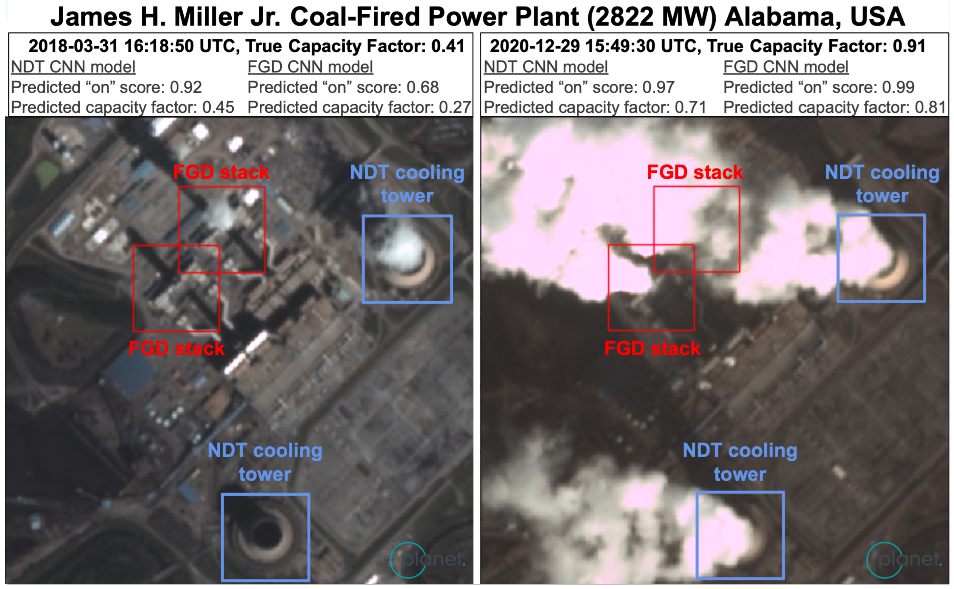
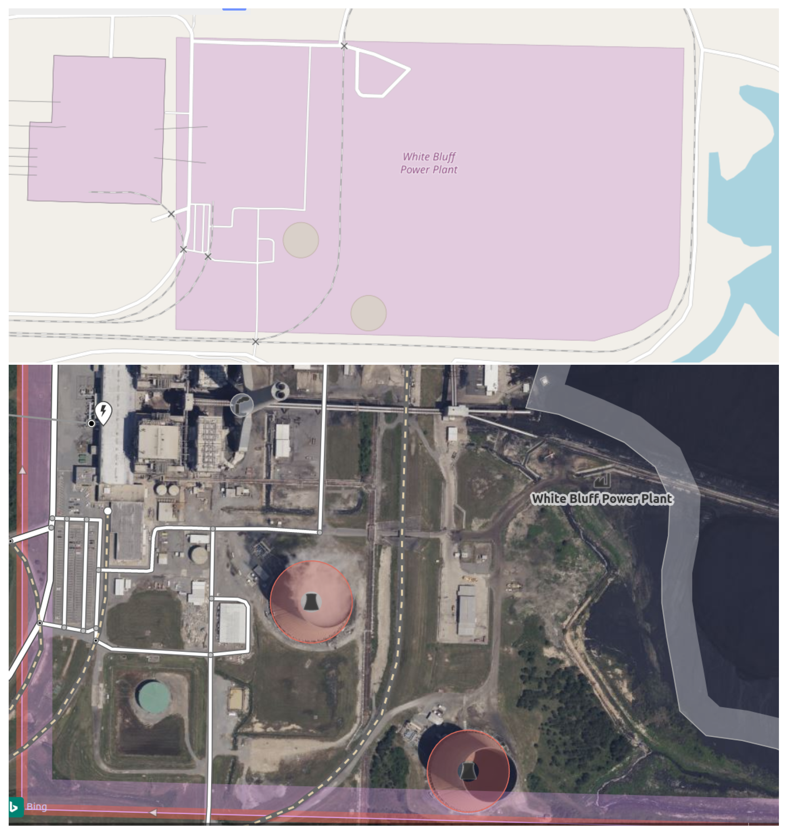
• Natural draft cooling towers (NDT): Plants using NDT have a large hyperbolic structure that allows vapor plumes to form during evaporative cooling.
• Wet flue gas desulfurization (FGD): After desulfurization, flue gases become saturated with water, increasing the visibility of plumes from the flue stack.

• In terms of size, NDT plumes are generally larger and wider than FGD plumes, making them easier to see in multi-spectral satellite imagery, as shown in Figure 1. A power plant may have one, both, or neither of these technologies. Due to the differing plume sizes and shapes from their sources, we created separate NDT and FGD models.

Observing the visible emitted water vapor plumes in multi-spectral satellite imagery, we built an ML modeling pipeline using gradient-boosted decision trees and convolutional neural networks (CNNs), and then trained these ML models to infer a power plant’s operational status. Specially, we designed models to perform two tasks:

• Sounding-level models: consist of (A) a classification model to classify whether a plant was running or not (on/off), and (B) a regression model to predict the capacity factor (i.e., what proportion of the power plant’s generation capacity was being used to generate power, generally between 0 and 1), for a given a satellite image of that plant at a certain point in time.
• Generation models: aggregate the predictions from the sounding-level models into the estimates of a power plant capacity factor over the preceding 30 days.

Each sounding model was trained on satellite images paired with the reported generation status. After predicting the capacity factor, it was multiplied by capacity (maximum electric power output) to infer generation. Our models are trained on power plants in countries for which we have hourly or sub-hourly generation data, which can be closely matched to the satellite image timestamp. Then, the models were applied globally using country-, fuel-, and prime-mover-specific average carbon intensities to convert the modeled plant-level generation into emission estimates. Figure 2 provides an overview of how these different models and data sources are integrated to estimate emissions.

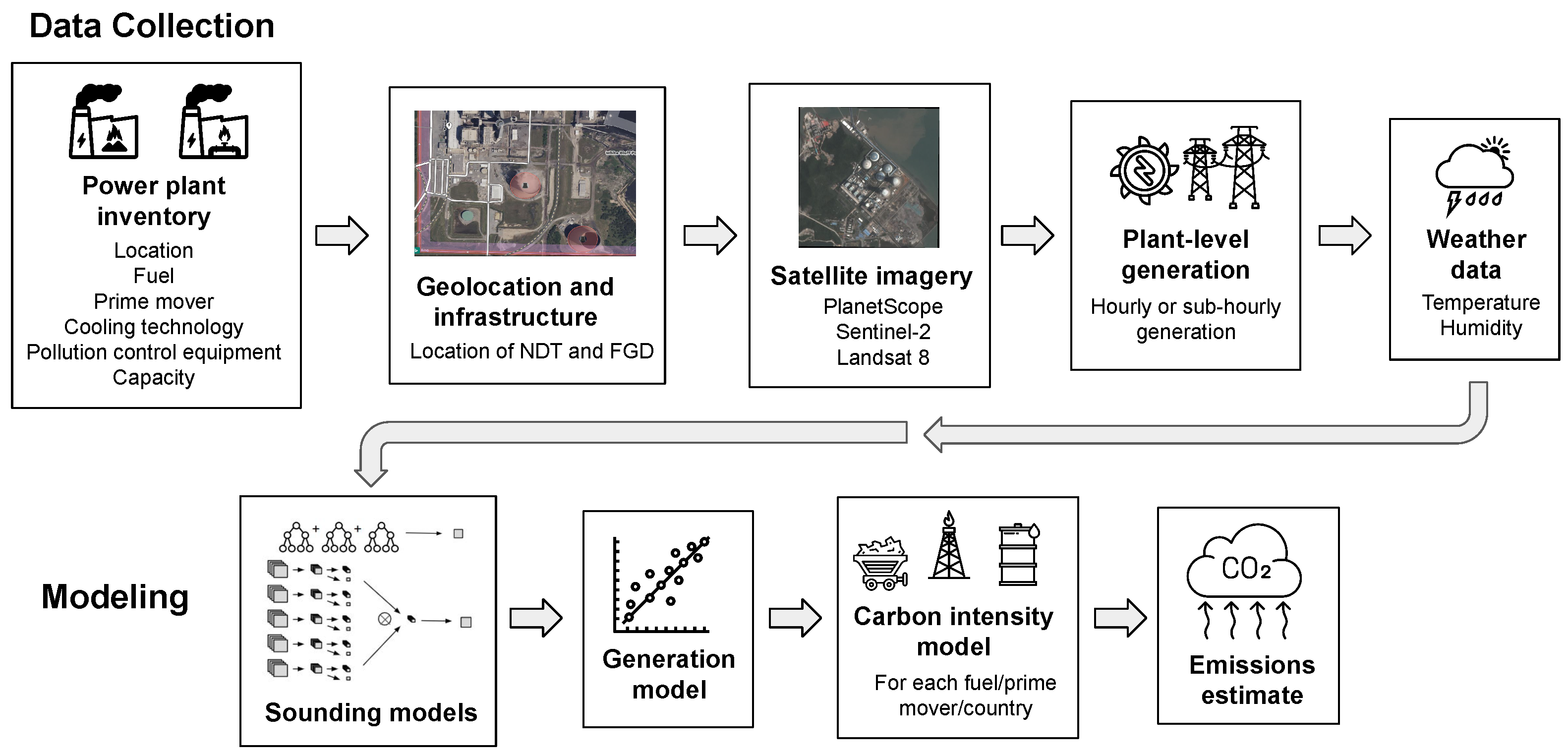
3.1. Power Plant Datasets

In order to form a set of power plants for training our model and running inference, we partnered with Global Energy Monitor (globalenergymonitor.org, accessed on 1 June 2023) to create a complete-as-possible, harmonized inventory of global combustion power plants that are currently operational. This was necessary because no single existing power plant dataset contains all the required information for this work. To use a plant in our ML modeling, we required the following inventory and auxiliary data:

• An accurate plant location for our satellite imagery.
• The location of FGD flue stacks and NDT cooling towers to focus our models on the relevant signals.
• Attributes of the power plant, including type, fuel, cooling technology, and air pollution control equipment to identify whether the plant is suitable for our models.
• Local weather data to decide whether temperature and humidity are conducive to vapor plume visibility.
• Plant capacity to determine whether the plant is of sufficient size to be modeled and to calculate the generation from the modeled capacity factor. This is used in conjunction with unit operating dates to find the plant capacity on any given date.
• Fuel and prime mover (i.e., steam or gas turbine) type to estimate the emissions factor.

In addition, plant-level electricity generation data is required for model training. Plants without generation data were used for inference only. We elaborate on each of these data requirements and our sources in Appendix A.

3.2. Satellite Data and Processing

Remote sensing imagery from the PlanetScope constellation, Sentinel-2A/B, and Landsat 8 satellites were employed in our ML modeling approach to infer a power plant’s operational status through the identification of emitted visible water vapor plumes. A sample image of a power plant from each satellite is shown in Figure 3. A description of each satellite and imagery processing step is provided below.

PlanetScope. Planet Labs’ PlanetScope satellite constellation consists of approximately 130 individual satellites, called “Doves”, with the first launch of this constellation in 2014 [35]. The PlanetScope constellation provides daily revisits with an equatorial crossing time between 7:30 and 11:30 a.m. (Planet, 2022). Each PlanetScope satellite images the Earth’s surface in the blue, green, red, and near-infrared (NIR) wavelengths (∼450–880 nm), with the exception of the “SuperDove” instrument which includes additional wavelengths [36,37]. The swath width is 25 km. PlanetScope PSScenes were downloaded via the Planet Labs API, providing a spatial resolution of ∼3 m, and including eight additional Usable Data Mask (UDM2) image quality bands.

Sentinel-2. The European Space Agency’s Sentinel-2 mission comprises two satellites: Sentinel-2A launched in 2015 and Sentinel-2B launched in 2017 [38,39]. Each Sentinel-2 satellite has a 10-day revisit time with a 5-day combined revisit and an equatorial crossing time of ∼10:30 a.m. [40]. Both satellites are equipped with a multispectral (MSI) instrument that provides 13 spectral band measurements, blue to shortwave infrared (SWIR) wavelengths and (∼442 nm to ∼2202 nm) reflected radiance and, depending on the band, provides measurements at 10 m–60 m spatial resolution [39,40]. The swath width is 290 km. We downloaded Harmonized Sentinel-2A/B Level-1C Top of Atmosphere (TOA) products from Google Earth Engine (GEE).

Landsat 8. The Landsat 8 mission was built and launched by NASA and is operated by US Geological Survey (USGS) [41,42]. Landsat 8 was launched in 2013 and has a 16-day revisit with an equatorial crossing time of 10 a.m. (+/− 15 min). Landsat 8 is equipped with two instruments: Operational Land Imager (OLI) and the Thermal Infrared Sensor (TIRS). OLI has nine spectral bands ranging from ∼430 nm to ∼1380 nm with a spatial resolution of 30 m. TIRS has two bands spanning 10,600 to 12,500 nm with a spatial resolution of 100 m that is upscaled to 30 m. [43]. The swath width is 185 km. We downloaded the Landsat 8 Collection 2, Tier 1 TOA from GEE.

Each satellite has multiple bands with different spatial resolutions. Lower-resolution bands were upsampled to match the highest-resolution band for that satellite. Each band also has a different distribution of pixel values, which can cause instability during model training. For this reason, we standardized the radiance values in each band to a mean of 0.5 and a standard deviation of 0.25, placing most pixel values between 0 and 1.

For some of our models, we created additional bands through post-processing:

• Haze-optimized transformation (HOT), a linear combination of the blue and red bands:

  $$\mathrm{HOT}=\mathrm{blue}-0.5\ast \mathrm{red}$$
• Whiteness [44], which consists of:

  $$\mathrm{whiteness}=\frac{|\mathrm{blue}-\mathrm{visible}|+|\mathrm{green}-\mathrm{visible}|+|\mathrm{red}-\mathrm{visible}|}{\mathrm{visible}}$$

  where $\mathrm{visible}=\frac{1}{3}(\mathrm{blue}+\mathrm{green}+\mathrm{red})$
• Normalized difference vegetation index (NDVI), a ratio between the red and near-infrared (NIR) bands,

  $$\mathrm{NDVI}=\frac{\mathrm{NIR}-\mathrm{red}}{\mathrm{NIR}+\mathrm{red}}$$
• Normalized difference shortwave infrared, a ratio between the shortwave infrared (SWIR) bands,

  $$\mathrm{normalized}\mathrm{difference}\mathrm{SWIR}=\frac{\mathrm{SWIR}2-\mathrm{SWIR}1}{\mathrm{SWIR}2+\mathrm{SWIR}1}$$
• Normalized difference thermal infrared, a ratio between the shortwave infrared (TIR) bands,

  $$\mathrm{normalized}\mathrm{difference}\mathrm{TIR}=\frac{\mathrm{TIR}2-\mathrm{TIR}1}{\mathrm{TIR}2+\mathrm{TIR}1}$$

These were generated for the satellites that have these available bands, i.e., normalized difference SWIR for Landsat 8 and Sentinel-2 but not for Planet. The band combinations provided additional beneficial features for some of our models. For example, HOT and whiteness acted as a basic plume mask. Our gradient-boosted tree models used all these bands, while the neural networks were more limited because of transfer learning, as described in Section 3.5. Additional uses of these synthetic bands for image selection will be detailed in Section 3.4.

3.3. Ground Truth Labels for Model Training

To train our ML models, our satellite images needed to be linked to plant-level generation data. We used satellite image timestamps to match each image to the nearest record of plant-level generation data, as described in Appendix A.4. Our training plants are located in the US, Europe, and Australia. For regression models, each satellite image was labeled with the capacity factor at that timestamp: the generation of the plant divided by its capacity at the given timestamp (see Figure 1). For classification, we labeled plants with a greater than 5% capacity factor as “on” and everything else as “off”. We used this nonzero threshold because there are a handful of plants reporting very low levels of generation that can functionally be considered “off”.

3.4. Plant and Image Selection

For all satellite imagery, a region of interest (ROI) was produced for each power plant by setting an outer boundary that envelops the plant itself, all associated facilities, and any other affected areas of interest. Based on this ROI, we restricted the training data to optimize for both modelability and impact:

• Plant selection. The first set of filters was based on the capacity of the plant and whether it was using mostly NDT or FGD technology at the time:
  • Coal must account for at least 50% of the plant’s operating capacity.
  • For NDT models, ≥70% of the plant’s cooling was NDT.
  • For FGD models, ≥90% of total generation and 100% of coal capacity was associated with wet FGD.
  • At least one NDT tower or FGD-enabled flue stack has been annotated in OpenStreetMap or in our in-house annotations database.
  • Capacity must be at least 500 MW.
  • Exclude from training any plants with incomplete or erroneous generation and/or retirement date, for example, failure to report generation for operating units, reporting generation several months past retirement, or insufficient or inconsistently reported generation data. This criterion is applicable to training only.
  • Because our modeling approach assumes that plants with wet FGD always run their pollution controls, we removed from training any operational plants that repeatedly exhibited sporadic or no visible FGD usage when the plant was reported “on”. For inference, this is harder to assess in the absence of reported generation data. We flagged operational plants with FGD where FGD plumes were never detected under the expected plume-favorable weather conditions (detailed later in this section) by our classification models, nor observed upon the manual inspection of 100 random images. We also flagged plants that exhibited other signals of operating (i.e., NDT plumes) with no FGD signal. There are two primary reasons for which an operational plant may fail to exhibit an FGD vapor plume signal when generating electricity under the appropriate temperature and humidity conditions:

    –

    Our power plant database has incorrect information suggesting that the power plant has a “wet” process when it is actually “dry”. This is possible for both NDT and FGD as either can be a “wet” or “dry” process; generally “dry” is more common in arid climates to conserve water.

    –

    The power plant fails to run its SOx pollution control equipment (the flue gas desulfurization, FGD), so there is no FGD plume. Note that this is only relevant for FGD plumes, not NDT, because some type of cooling is necessary to operate a power plant, whereas pollution controls are not strictly necessary to operate (rather, they represent additional requirements set by clean air regulations).

  For inference on NDT plants, these criteria were relaxed by applying our models to all the plants that met the following criteria every year: a total capacity of at least 50 MW and any positive amount of NDT capacity, regardless of fuel type. Despite the loosened criteria, the vast majority of plants in our external validation sets for both electricity generation and emissions burn >50% coal.
• Image selection. We also filtered based on the characteristics of each satellite image:
  • Our FGD and NDT annotations are fully contained within the satellite image.
  • The cloud mask over the plant indicated <20% cloud coverage. This threshold is set relatively high to avoid falsely excluding images containing large plumes, which are easily misclassified as clouds.
  • For PlanetScope, we used the post-2018 UDM2 bands to keep only images with <80% heavy haze.
  • For all PlanetScope images, we calculated the mean brightness and developed a cloudiness score based on HOT, whiteness, and NDVI, respectively, to filter out excessively dark or cloudy images.
  • Images with known data quality issues were discarded, e.g., exhibiting plumes when generation has been zero for at least an hour. Appendix A.4 details the scenarios in which we excluded images due to quality issues.
  • When there were images of the same location with the same timestamp, we kept a single copy, breaking ties with the following: (1) largest area surrounding the plant contained; (2) least cloudy area; (3) latest download timestamp; and (4) random selection.
• Weather filters. Ambient temperature and relative humidity were obtained for each plant as detailed in Appendix A.3. Images were excluded from FGD models when ambient weather conditions were unfavorable for plume visibility. At high temperatures and/or low relative humidity, the water vapor in the flue stack does not readily condense, plume visibility is reduced, and our models have no signal to detect. The warmer the temperature, the more humid it needs to be for water vapor plumes to be visible, eventually becoming very faint at high temperatures regardless of the humidity. At colder temperatures, however, even very dry conditions will still result in a visible plume. Therefore, we used empirically derived cutoff rules for plume visibility:
  • Exclude images in which the ambient temperature is ≥14 °C and relative humidity is ≤26%.
  • Exclude images in which the ambient temperature is ≥24 °C and relative humidity is ≤36%.
  • Exclude images in which the ambient temperature is ≥32 °C.

After applying the above plant, image, and weather filters, our training dataset consisted of 74 plants for NDT and 99 for FGD during the years 2015–2022.

Table 1. Training image count for the years 2015–2022 for each satellite before and after filtering. For PlanetScope, we applied cloud filtering prior to downloading images, so the “Before filtering” column does not include cloudy images. Note that the same image may be used by both the NDT and FGD models since a power plant can have both types of technology.

Satellite	NDT Image Count		FGD Image Count
	Before Filtering	After Filtering	Before Filtering	After Filtering
PlanetScope	69,533	54,136	108,038	69,462
Sentinel-2	18,964	15,064	30,541	18,390
Landsat 8	9040	7176	12,885	8235

lists the number of training images for each satellite before and after filtering.

3.5. Sounding Models

To estimate power plant generation and CO₂ emissions from satellite imagery at a specific timestamp, our sounding-level models predicted whether a power plant was running or not (on/off) and estimated the capacity factor (generation divided by capacity). We included both sets of models because the on/off task was simpler and could be predicted more accurately, while the regression task was essential for differentiating low from high generation. We multiplied the predicted capacity factor by the capacity to infer generation.

As we estimate power plant activity by identifying vapor plumes, focusing our models on the structures that emit these plumes can improve performance. Therefore, we used the annotated NDT cooling tower and FGD stack patches as model inputs, as shown by the red and blue boxes in Figure 1. This helped produce more accurate classification models than a single image of the entire plant, which can have the features of non-power plant activity impacting the accuracy [33]. Two different types of models were trained: gradient-boosted decision trees and convolutional neural networks (CNNs). For each model type, separate models for NDT and FGD were built, as well as for each satellite dataset, for a total of 16 sounding models. Figure 4 illustrates the structure of both model types.

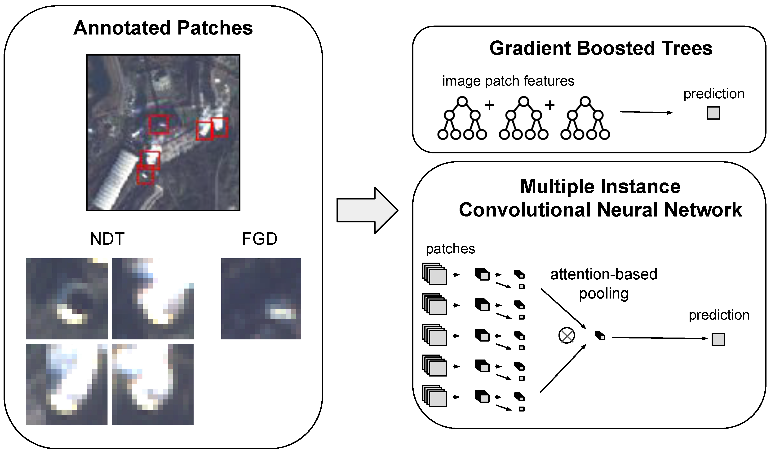
3.5.1. Gradient-Boosted Decision Trees

The gradient-boosted decision tree models used XGBoost. For each image fed into the XGBoost models, we extracted the patches of varying sizes centered on the FGD or NDT structures. A set of statistics was derived for the pixel values in each patch: mean, standard deviation, and 90th percentile. These vectors of statistics were then aggregated to the image level using mean, min, and max operations to accommodate the plants with multiple FGD or NDT structures. We used multiple patch sizes around the FGD or NDT structures (4–32 pixels for Landsat 8, 4, to 32 pixels for Sentinel-2, and 8 to 64 pixels for PlanetScope) in order to capture features at different scales.

Visible plumes at power plants tend to be white. However, there can be other white features, such as buildings, near the cooling tower or flue stacks. To handle this, we also included features from background-subtracted images. Background images were calculated as the median pixel value across a random set of 32 images of the plant. The background images were then subtracted from the current image, and the same set of statistical features was calculated and concatenated to the previous set, as described above.

3.5.2. Convolutional Neural Networks

To enable the CNN models to handle multiple patches, we used a multiple instance framework to combine patches via an attention layer, with the patch size being tuned as a hyperparameter (hyperparameters are discussed in greater detail in Section 3.8). The attention mechanism aggregates the features from all the different patches for a particular image of a plant [33,34]. Each patch was first encoded with a CNN encoder truncated after a subset of the convolutional blocks. Transfer learning was used to initialize model weights in one of two ways:

• RESISC: a ResNet50 CNN [45] pre-trained on the RESISC dataset, which consists of aerial RGB images labeled by land cover and scene classes [46]. The RESISC dataset is particularly relevant because it includes a cloud class, enabling the model to capture distinguishing features of clouds—and, likely, plumes. This model uses the RGB channels only.
• BigEarthNet: with a VGG16 CNN [47] pre-trained on the BigEarthNet dataset, which consists of Sentinel-2 images labeled by land cover class [48]. This model uses 10 bands from Sentinel-2, excluding the lowest resolution bands of 1, 9, and 10. We were not able to apply this model to PlanetScope but did adapt it for Landsat 8 by matching the band wavelengths as closely as possible and pairing the remaining bands even if the wavelengths are different. While this dataset enabled the model to learn a more diverse set of spectral characteristics, it only contained cloud-free images; our model must learn plume features during fine-tuning.

After the shared convolutional encoder, we used an attention layer to combine patch features as a weighted sum, with the weights determined by the model itself [49]. A dense layer then made the final prediction. More details about model configuration and training are provided in Appendix B.

3.6. Generation Ensemble Models

The sounding-level models described in Section 3.5 give us an instantaneous estimate of the power plant activity in a single satellite image. Collecting these instantaneous estimates creates an irregular time series of on/off classification and capacity factor regression estimates for each plant. In order to estimate emissions of a plant over a given period of time, we built a set of second-stage models (“generation models”) responsible for aggregating the sounding model time series into features and predicting a rolling 30-day average capacity factor for each plant (predicting one value for each day, that value being the average capacity factor over the preceding 30 days). We then multiplied this capacity factor with each plant’s capacity to obtain the plant’s estimated generation. Afterward, the estimated generation was multiplied by an emissions factor, as described later in Section 3.7, to estimate emissions.

Separate generation models were trained for NDT and FGD plants and only for the years 2018 to 2022 inclusive. This is because there is very limited PlanetScope data available prior to 2018, making rolling 30-day predictions difficult due to the sparsity of soundings. Each generation model is an L1-regularized linear regression model with features formed from aggregating the sounding model predictions (described in Appendix C). To calculate features for each plant at each point in time, we aggregated the predictions from the sounding-level models over multiple lookback windows. In total, the NDT model had access to 162 features, while the FGD model had access to 324 features (see Appendix C for the list of features). All features were standardized to a mean of zero and unit standard deviation prior to model training. The same standardization factors were applied for inference.

The lookback windows over which we aggregated predictions for the NDT generation model were 30, 60, and 180 days. Due to the lower number of soundings for the FGD generation model, its lookback windows were 30, 60, and 365 days. In addition to including more plant-specific information, these longer windows also allowed our models to account for the longer-term behavior of the plant when making a prediction. The generation models were trained with L1-regularization weights of 0.01 and 0.005 for FGD and NDT, respectively. Figure 5 shows an example of FGD and NDT model predictions compared with the capacity factor calculated from reported electricity generation.

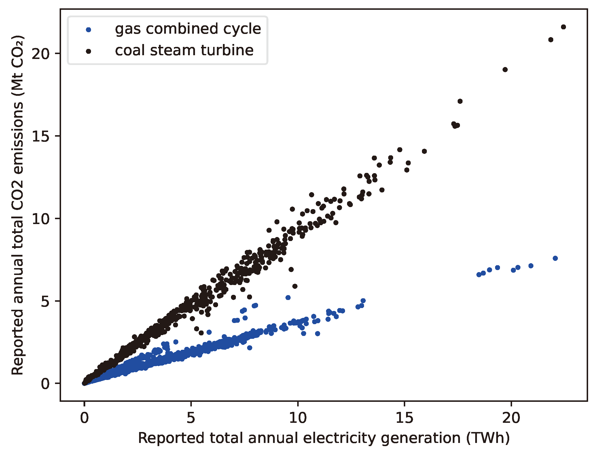
3.7. Emissions Estimation

To generate plant-level emissions estimates, we first estimated the annual capacity factor of each plant. Then, the rolling 30-day average capacity factor estimates were converted into the annual capacity factor by averaging and weighting each estimate by what fraction of the 30-day interval fell into the year in question. The total unit level annual generation is the product of (1) the hourly capacity factor, (2) the unit capacity, and (3) the number of hours in the year. The unit-level annual emissions are the product of (1) the generation and (2) the carbon intensity (see Appendix A.6). Finally, the unit-level estimates were aggregated to the plant level to provide the annual facility-level emissions estimate.

3.8. Model Training with Cross-Validation

As our goal was to estimate the power plant emissions when no reported generation data exist, it is essential to validate that our models generalize well to unseen plants. To do this, we used cross-validation, a resampling procedure in which the data are divided into a set of folds, and models are iteratively trained and tested on different subsets of these folds. We built a regular $1^{\circ }\times 1^{\circ }$ grid in latitude–longitude space and placed plants in the same grid cell into the same fold. Each plant was assigned to a single fold, with all of its images belonging to that same fold. By rotating the assignment of these folds to training/tuning/testing, we were able to train and evaluate four different models. For each one, two of the four folds of plants were used for training, one for tuning/validation, and one for testing. The details of model training are specified by hyperparameters such as patch size and learning rate. We independently tuned the hyperparameters of both XGBoost and CNN models to optimize for validation mean average precision (mAP) and root mean squared error (RMSE) for classification and regression, respectively. We selected mAP due to the class imbalance; plants were “on” in about ∼80% of the training images.

Since the generation models are trained on the outputs of other ML models—the sounding models—we must take extra care to prevent the use of information from model training that would not be available at the prediction time, i.e., data leakage. Therefore, the following cross-validation approach was adopted for the training and evaluation of the generation models. Each of the four generation model instances was trained with features based on soundings from the validation fold and evaluated with features based on the sounding predictions from the testing fold. This way, both sets of sounding predictions come from the same sounding model and were not used for its training. While the sounding models might be overfitted to their validation fold due to early stopping and hyperparameter tuning, the test fold was not used for any model optimization or selection. Thus, measuring the performance on the test fold provides a reasonable representation of predictions on unseen plants.

3.9. Model Inference

To produce our final generation estimates, we followed the same data processing steps laid out in the previous sections, but with relaxed filters as described in Section 3.4.

Predictions for all images were generated during the period 2015–2022, using our sounding-level models described in Section 3.5. For inference, the sounding predictions were averaged from all four instances of a sounding model (one model for each fold). Then, these predictions were converted to generate time series features and rolling 30-day average capacity factor predictions using the generation models as described in Section 3.6. Similarly to the sounding models, the predictions were averaged from all four instances of a generation model to obtain the final generation prediction. The result is a set of predictions, one per day per plant, of the average capacity factor of that plant over the preceding 30 days. These were then summed and weighted by how much the 30-day interval overlaps with the year to produce the estimates of the annual plant-level capacity factor.

The sounding and generation models were run on NDT and FGD structures separately to estimate the activity of the entire plant. For plants that have only FGD or only NDT, the estimation process was straightforward: simply use the prediction from the single applicable model. For plants with both NDT and FGD, predictions were aggregated from both model types by weighting the NDT model prediction two times more than the FGD model prediction ($\frac{2\ast \mathrm{NDT}+\mathrm{FGD}}{3}$), reflecting the lower error and increased confidence in the NDT models.

4. Results

We used two mechanisms to validate our models. First, through cross-validation on our training set, performance was measured on the held-out fold and aggregated across the four folds (details in Section 3.8). Second, additional generation and emissions data were gathered from plants with NDT and/or FGD in Türkiye (not reported to ENTSO-E or EU ETS with the rest of Europe) and India (Appendix A.4 and Appendix A.5), plus plants with NDT in the US, Europe (reported to ENTSO-E or EU ETS), and Australia that did not meet our strict filters for training but did qualify with a looser filter due to a lower capacity or a more heterogeneous set of cooling types (Section 3.4). We refer to the first mechanism on training plants as “cross-validation” and the second on non-training plants as “external validation”.

Table 2. Coverage summary of Climate TRACE’s ML approach, as compared with prior work discussed in Section 2; all studies that included ten or more plants are listed. Percent power emissions are calculated per year, and then averaged to produce the value in the table, using as a denominator the total power sector emissions, as estimated by Climate TRACE for each year (note that the ML technique presented in this paper represents just one of the ways that Climate TRACE estimates power sector emissions [51]).

Approach	% Power Emissions	# Observations	# Plants	# Countries	Years
Climate TRACE ML
Cross-val	7%	157,831	139	12	2015–2022
External val (generation)	2%	107,440	101	16	2018–2022
External val (CO2)	7%	162,588	207	17	2019–2022
All inference	32%	1,198,167	1042	41	2015–2022
Jain [32]	<1%	2131	146	18	2019–2021
Hanna et al. [31]	<1%	1639	146	11	2020
Lin et al. [15] inference	4%	106	78	15	2018–2021
Lin et al. [15] validation	<1%	50	22	1	2018–2021
Cusworth et al. [7]	<1%	28	21	4	2014–2020
Nassar et al. [12]	<1%	20	14	6	2014–2018

below summarizes the fraction of the total power sector emissions and the number of observations, plants, and countries to which we applied our ML methods, as compared to prior work we discussed in Section 2. We validated our methodology on nearly twice as many plants, with two-to-four orders of magnitude more observations, and a broader selection of countries than any prior study. Furthermore, our inference predictions encompass 1042 power plants across 41 countries, including several plants in each of the five countries that produce the most carbon emissions from power generation (in order): China, US, India, Russia, and Japan [50]. Figure 6 displays the coverage of our emission estimates for 2022 on a map.

Using these two mechanisms, cross-validation and external validation, the performance was evaluated for our sounding, generation, and emissions models. The results are detailed in this section. We also calculated 90% confidence intervals by block bootstrapping the test set (blocking on plants, i.e., resampling plants rather than images to ensure plants were not split up).

Our validation sets consist of combustion power plants with NDT and/or FGD technologies. Few plants burn exclusively one type of fuel; most use a variety of types. Plants that use NDT may have any variety of fuel mix, even 0% coal, but plants with FGD all burn some amount of coal because the purpose of FGD is to remove the SO₂ emitted when coal is burned. The vast majority of plants in our validation sets burn some amount of coal. Of the 207 plants in our emissions validation dataset, 16 (8%) did not burn any coal since 2016. These 16 plants all burn mostly gas, with oil or waste heat filling the gaps (no biomass). There are two plants that burn biomass in this emissions validation dataset; however, both still burn mostly coal.

4.1. Sounding Model Validation

Classification and capacity factor regression results for the period 2015–2022 are displayed in

Table 3. On/off classification cross-validated mean average precision (mAP) and block-bootstrapped 90% confidence intervals for 2015–2022.

Satellite	Model	NDT mAP [CI]	FGD mAP [CI]
PlanetScope	XGBoost	0.956 [0.932, 0.987]	0.886 [0.857, 0.911]
PlanetScope	CNN-RESISC	0.930 [0.901, 0.963]	0.885 [0.861, 0.916]
Sentinel-2	XGBoost	0.932 [0.904, 0.980]	0.889 [0.858, 0.917]
Sentinel-2	CNN-RESISC	0.959 [0.941, 0.974]	0.903 [0.880, 0.925]
Sentinel-2	CNN-BigEarthNet	0.933 [0.906, 0.966]	0.839 [0.801, 0.873]
Landsat 8	XGBoost	0.899 [0.866, 0.942]	0.878 [0.855, 0.904]
Landsat 8	CNN-RESISC	0.901 [0.866, 0.942]	0.824 [0.793, 0.854]
Landsat 8	CNN-BigEarthNet	0.865 [0.826, 0.899]	0.811 [0.784, 0.837]

and

Table 4. Capacity factor regression cross-validated root mean squared error (RMSE) and mean bias error (MBE), alongside respective block-bootstrapped 90% confidence intervals, for 2015–2022.

Satellite	Model	NDT		FGD
		RMSE [CI]	MBE [CI]	RMSE [CI]	MBE [CI]
PlanetScope	XGBoost	0.209 [0.194, 0.221]	−0.021 [−0.034, −0.006]	0.297 [0.285, 0.308]	−0.056 [−0.076, −0.037]
PlanetScope	CNN-RESISC	0.196 [0.186, 0.206]	−0.024 [−0.037, −0.010]	0.263 [0.244, 0.277]	−0.065 [−0.084, −0.045]
Sentinel-2	XGBoost	0.210 [0.198, 0.220]	−0.020 [−0.034, −0.006]	0.270 [0.258, 0.281]	−0.029 [−0.049, −0.011]
Sentinel-2	CNN-RESISC	0.203 [0.192, 0.213]	−0.019 [−0.034, −0.004]	0.267 [0.248, 0.282]	−0.048 [−0.066, −0.029]
Sentinel-2	CNN-BigEarthNet	0.220 [0.206, 0.233]	−0.025 [−0.041, −0.008]	0.259 [0.246, 0.269]	0.005 [−0.014, 0.025]
Landsat 8	XGBoost	0.243 [0.220, 0.260]	−0.011 [−0.032,  0.013]	0.285 [0.271, 0.298]	−0.063 [−0.085, −0.042]
Landsat 8	CNN-RESISC	0.266 [0.249, 0.280]	−0.089 [−0.110, −0.068]	0.299 [0.289, 0.309]	−0.036 [−0.054, −0.015]
Landsat 8	CNN-BigEarthNet	0.264 [0.247, 0.278]	−0.031 [−0.054, −0.006]	0.301 [0.288, 0.313]	0.025 [0.002, 0.050]

, respectively. A naive baseline mAP is 0.5 for a model that predicts the most prevalent class, or always “on”. This serves as a simple benchmark against which to compare our models’ performance. For the regression model, a naive baseline that predicts a constant value of the training set’s mean capacity factor would produce an RMSE of 0.34 and a mean bias error (MBE) of 0 across all imagery sources for both NDT and FGD. Models were trained and cross-validated on 99 plants with FGD (25 in Europe’s ENTSO-E and 74 in the US) and 74 plants with NDT (45 in Europe’s ENTSO-E, 22 in the US, and 7 in Australia). All of our models outperformed their respective baselines—and by an especially wide margin on the simpler task of classification. NDT models generally did better than FGD because NDT tends to produce larger plumes.

Comparing the different model types drew out a few more insights. The BigEarthNet models require 10 bands and so can only be used for Sentinel-2 and Landsat 8. In general, RESISC models performed slightly better than BigEarthNet. Overall, RESISC and XGBoost fared similarly, with RESISC sometimes outperforming XGBoost and sometimes vice versa, emphasizing the utility of an ensemble approach. Both PlanetScope and Sentinel-2 models performed similarly; the on/off classification mAP for both varied from 0.93 to 0.96 for NDT and from 0.84 to 0.90 for FGD across all models, and the capacity factor regression RMSE for both ranged from 0.20 to 0.22 for NDT and 0.26 to 0.30 for FGD. The Landsat 8 models generally were less accurate, with on/off classification mAP values of 0.81 to 0.90, and capacity factor regression RMSE values between 0.24 and 0.30. The Landsat 8 models’ lower performance is most likely due to the coarser 30 m spatial resolution and revisit rate of 16 days, which results in fewer training images. Additionally, the capacity factor regression RMSE values for Sentinel-2 and PlanetScope overlap, which suggests that Sentinel-2’s 10 m resolution is sufficient to identify on/off classification and the capacity factor. Even though PlanetScope’s 3 m resolution did not substantially improve the model’s performance, the daily revisits improve the temporal resolution, allowing for the more frequent capturing of the on/off and capacity factor identification at power plants, which produces a greater number of total observations in each year.

Appendix D includes some additional results validating our sounding models on non-training plants in the US, Europe (ENTSO-E), Australia, and Türkiye. On these plants, our NDT classification models using Sentinel-2 and PlanetScope imagery performed similarly with an mAP between 0.74 and 0.78, while the Landsat 8 models received lower average classification mAP scores of ∼0.72. These NDT classification results are worse than the cross-validation performance but are still significantly (alpha = 0.1) better than a naïve baseline of 0.5 mAP. The NDT regression models’ overall average performance was 0.22, 0.23, and 0.27 for PlanetScope, Sentinel-2, and Landsat 8 models, respectively, which is comparable to the cross-validation performance above. For the FGD model validation, only three plants with FGD had reported data available to compare against, but a similar trend was seen as the Sentinel-2 and PlanetScope models performed better than the Landsat 8 models.

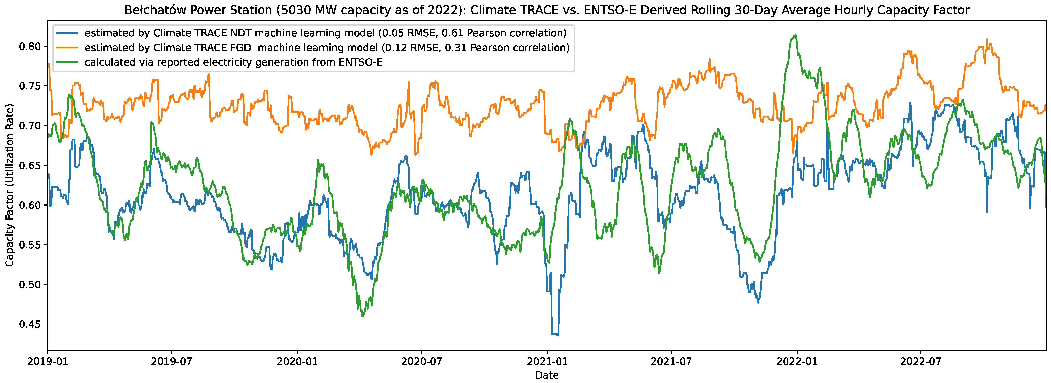
4.2. Generation Model Validation

To validate our generation models, we measured performance using the RMSE between the reported and predicted 30-day rolling average capacity factors in the validation set.

Table 5. Generation ensemble model performance for each plant type, during the period of 2018–2022, for training plants using cross-validation and on additional plants as external validation. Baseline results and a 90% confidence interval are also included.

Plant	Validation	Plant	RMSE		MBE
Type	Type	Count	ML [CI]	Baseline	ML [CI]	Baseline
NDT	cross	73	0.149 [0.129, 0.162]	0.272	−0.014 [−0.028,  0.002]	0.000
NDT	external	104	0.199 [0.188, 0.210]	0.273	−0.075 [−0.091, −0.058]	0.048
FGD	cross	97	0.196 [0.187, 0.205]	0.270	0.012 [−0.007, 0.031]	0.000
FGD	external	4	0.323 [0.216, 0.384]	0.359	−0.252 [−0.330, −0.127]	−0.272

summarizes the results of our two generation models for both cross-validation (training plants in the US, Europe (ENTSO-E), and Australia) and external validation (non-training plants in the US, Europe (ENTSO-E), Australia, Türkiye, and India). While we included imagery from as early as 2015 for the sounding model, we focused on 2018–2022 for the generation model. This is because PlanetScope has limited imagery before 2018, and this higher-temporal-resolution is crucial for predicting the 30-day rolling capacity factor. The baseline used is again the average value of the target in the relevant training set, i.e., the average capacity factor: 0.44 for NDT plants and 0.47 for FGD plants. Compared to the sounding-level regression tasks described previously, the NDT ensemble model lead to a lower baseline RMSE of 0.27. This is due to the smoothing effect from 30 to day averaging. Our generation ensemble models combine multiple sounding model types, satellite imagery sources, and timescales to outperform this baseline significantly (alpha = 0.1) with an RMSE of 0.149 to 0.199 in almost all cases for both cross-validation and external validation. The one exception is FGD external validation, which was based on only four plants (due to limited reported data) that produced an RMSE of 0.323. These four plants include the same three in Türkiye used for sounding validation and one additional plant in India.

Limited conclusions can be drawn from the external validation on FGD plants, as there are only four plants with reported data in this group. Sounding-level FGD results for Türkiye showed both a high RMSE and a large negative MBE (

Table A3. On/off classification and regression external validation on 3 FGD plants in Türkiye, 2015–2022.

Satellite	Model	Classification	Regression
		mAP [CI]	RMSE [CI]	MBE [CI]
PlanetScope	XGBoost	0.664 [0.531, 0.909]	0.487 [0.463, 0.504]	−0.373 [−0.416, −0.323]
PlanetScope	CNN-RESISC	0.778 [0.623, 0.943]	0.394 [0.392, 0.395]	−0.299 [−0.303, −0.295]
Sentinel-2	XGBoost	0.615 [0.519, 0.766]	0.455 [0.411, 0.492]	−0.350 [−0.407, −0.277]
Sentinel-2	CNN-RESISC	0.604 [0.523, 0.871]	0.461 [0.416, 0.500]	−0.356 [−0.410, −0.292]
Sentinel-2	CNN-BigEarthNet	0.682 [0.529, 0.940]	0.474 [0.444, 0.496]	−0.390 [−0.419, −0.346]
Landsat 8	XGBoost	0.586 [0.517, 0.765]	0.519 [0.444, 0.584]	−0.406 [−0.516, −0.296]
Landsat 8	CNN-RESISC	0.550 [0.517, 0.714]	0.509 [0.479, 0.543]	−0.400 [−0.477, −0.329]
Landsat 8	CNN-BigEarthNet	0.569 [0.568, 0.829]	0.430 [0.408, 0.447]	−0.318 [−0.372, −0.260]

). These errors are once again reflected in the results for our generation model (Table 5, bottom row).

Our generation models performed better on NDT than FGD plants, which is explained by both the better performance of the NDT sounding-level model as well as the reduced number of sounding-level predictions going into the FGD models due to the weather filters described in Section 3.4 that lead to periods with very little sounding-level information for some plants. These results also demonstrate that, by aggregating to a coarser temporal resolution (from hourly generation at the sounding level to rolling 30-day average generation), our error rate reduces substantially.

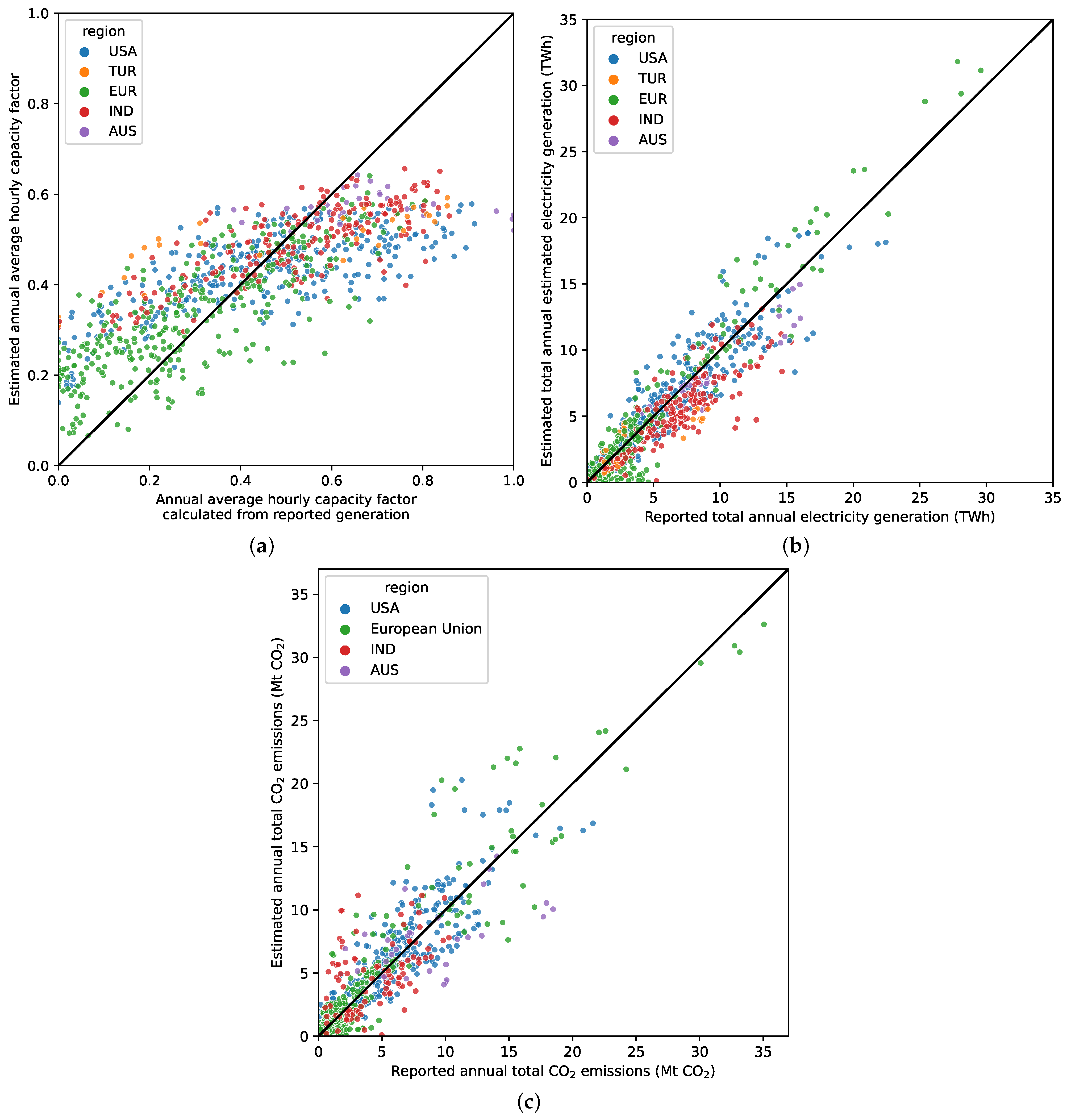
4.3. Annual Validation

Facility-level annual average capacity factor, total electricity generation, and total CO₂ emissions were calculated from the sounding and generation model outputs for 2019–2022, inclusive. This year range was selected because generation model training was restricted to 2018–2022 (due to the scarcity of PlanetScope data prior to 2018) and because of the overlapping nature of the 30-day windows and fiscal year differences necessitating lookbacks to the previous year.

In addition to our ML models, we produced a second set of simpler baseline capacity factor estimates. We used country-level annual estimates of capacity and generation by fuel type from the EIA (eia.gov/international/data/world/electricity/more-electricity-data, accessed on 1 May 2023) and EMBER (ember-climate.org/data-catalogue/yearly-electricity-data, accessed on 1 May 2023). From this, we calculated the annual average fuel-specific capacity factor in each year reported for each country in the world. We then assumed the same capacity factors within each country for each part of the plant with the associated fuel type. This does not account for the typical variation in dispatch for plants serving base, intermediate, and peaking loads. This baseline is different to those used in Section 4.1 and Section 4.2 which were simply calculated from the training data, whereas this one is based on country- and fuel-specific averages. Metrics were calculated by comparing the estimates derived from our ML methods to the reported generation data summarized in Appendix A.4 or emissions data summarized in Appendix A.6. We used this as a baseline rather than alternatives like EDGAR, ODIAC, or OCO-2/3 for the reasons described in Section 5.

Table 6. Annual average capacity factor estimation performance for 2019–2022 compared to the capacity factor derived from the reported generation data for the US, Europe, (ENTSO-E), Australia, India, and Türkiye, as reported by their respective government mechanisms summarized in Appendix A.4. A comparison to the country- and fuel-specific average baseline is also included.

Region	Validation	Plant	RMSE		MBE
	Type	Count	ML [CI]	Baseline	ML [CI]	Baseline
US	cross	78	0.17 [0.16, 0.18]	0.22	−0.02 [−0.05,  0.00]	−0.05
US	external	6	0.14 [0.12, 0.17]	0.19	0.03 [−0.06, 0.12]	0.04
Europe (ENTSO-E)	cross	59	0.12 [0.11, 0.13]	0.20	0.04 [0.02, 0.06]	0.05
Europe (ENTSO-E)	external	27	0.14 [0.12, 0.16]	0.18	0.02 [−0.01, 0.05]	0.10
Australia	cross	7	0.20 [0.08, 0.26]	0.18	−0.12 [−0.20, −0.04]	−0.10
Australia	external	1	0.09 [N/A]	0.09	−0.01 [N/A]	0.04
India	external	50	0.14 [0.13, 0.15]	0.20	−0.03 [−0.05, −0.01]	0.08
Türkiye	external	8	0.24 [ 0.21,  0.26]	0.32	0.00 [−0.12,  0.10]	0.13

displays performance metrics for the annual average capacity factor. For the US and Europe (ENTSO-E), cross-validation performance is comparable with an RMSE of 0.17 and 0.12, respectively, and external validation is 0.14 for both. The region with the highest (lowest performing) external validation RMSE was Türkiye with 0.24. The region with the largest MBE was Australia with -0.12. This may be due to Australian power plants generally running at higher capacity factors than the rest of the training set. The fifty plants in India, on the other hand, achieved results that are very similar to the US training plants, lending credibility to the generalizability of our ML emissions estimation approach.

Comparing modeled to reported annual generation and emissions for individual power plants, the overall RMSEs, aggregating across both cross- and external validation, were 1.75 TWh and 2.18 Mt CO₂, respectively.

Table 7. Annual total generation estimation performance compared to the reported generation data (in terawatt–hours, TWh) for the US, Europe (ENTSO-E), Australia, India, and Türkiye during the period 2019–2022.

Region	Validation	Plant	RMSE (TWh)		MBE (TWh)
	Type	Count	ML [CI]	Baseline	ML [CI]	Baseline
US	cross	78	1.68 [1.51, 1.84]	2.99	0.06 [−0.16, 2.90]	−0.65
US	external	6	2.92 [0.68, 3.92]	3.90	−0.66 [−2.17, 0.88]	0.31
Europe (ENTSO-E)	cross	59	1.38 [1.09, 1.58]	2.43	0.35 [0.15, 0.53]	−0.16
Europe (ENTSO-E)	external	27	1.39 [1.09, 1.61]	1.27	−0.55 [−0.82, −0.28]	0.65
Australia	cross	7	2.05 [ 0.91, 2.60]	2.19	−1.46 [−2.08, −0.63]	−1.33
Australia	external	1	1.12 [N/A]	0.94	−0.49 [N/A]	0.37
India	external	50	2.12 [1.78, 2.37]	2.58	−1.38 [−1.63, −1.12]	0.98
Türkiye	external	8	2.08 [1.31, 2.57]	2.80	−0.94 [−1.91,  0.01]	0.97

and

Table 8. Annual emissions estimation performance compared to the reported data for the US, EU, Australia, and India during the period 2019–2022.

Region	Validation	Plant	RMSE (Mt CO2)		MBE (Mt CO2)
	Type	Count	ML [CI]	Baseline	ML [CI]	Baseline
US	cross	77	2.11 [1.73, 2.36]	2.68	0.37 [ 0.08,  0.67]	−1.13
US	external	5	1.12 [0.37, 1.43]	2.25	−0.61 [−1.08, −0.10]	−0.56
EU	cross	58	2.27 [1.70, 2.68]	3.04	0.57 [0.19, 0.97]	−0.18
EU	external	36	1.00 [0.76, 1.16]	1.05	−0.41 [−0.58, −0.23]	0.25
Australia	cross	6	4.17 [2.91, 5.12]	3.67	−1.40 [−2.98, 0.34]	−0.84
Australia	external	1	3.23 [N/A]	2.63	−2.06 [N/A]	−1.21
India	external	24	2.74 [2.41, 3.01]	4.06	0.33 [−0.02, 0.68]	2.72

show the performance of our ML methods for annual total generation (in terawatt–hour or TWh) and annual CO₂ emissions (in megatonnes or Mt) estimation. For US cross- and external validation, Europe (ENTSO-E for generation and EU ETS for emissions) cross-validation only, and India and Türkiye (both exclusively external validation), the ML-based estimate had a significantly lower RMSE than the baseline approach using country averages. However, the RMSE for Europe (ENTSO-E for generation and EU ETS for emissions) external validation and all Australian plants was no better than the baseline approaches. Furthermore, for Australia, the errors were significantly worse than anywhere else with the ML-based method, underpredicting substantially. This may once again be because the ML models failed to capture the higher average utilization rate in Australia, which makes up a small percentage of training plants, relative to the lower average utilization rate of the rest of the training set. That being said, the overall plant-wise annual RMSEs of 1.75 TWh and 2.18 Mt CO₂ are small relative to the annual generation and CO₂ emissions of the world’s largest power plants, as can be seen in Figure 7, which plots our estimates for the average annual capacity factor, total annual generation, and annual CO₂ emissions at individual plants against reported electricity and emissions data.

In conclusion, although our models have an RMSE of 0.12–0.24 in terms of capacity factor, they are reliable in differentiating low versus high utilization. Validating against reported data, instead of remote sensing-derived GHG estimates discussed in Section 2, provides robust and more plentiful verification of specific plants. One area for improvement is that the model struggles to predict high-capacity factors, favoring mid-range predictions instead, which contributes to a negative bias in this range. However, once the total generation and emissions are calculated from our capacity factor estimates, and compared to reported values, the bias of our models is much more evenly distributed across plants with different total generation and emissions. Looking at our external validation results, our models underestimate the reported annual emissions the most in Australia (n = 7) where plants generally run at a higher capacity factor relative to the training regions according to reported generation data. On the other hand, the slight positive bias of emissions estimates in India (n = 24) is more in line with the US and Europe (EU ETS), lending credibility to the generalizability of our ML emissions estimation approach beyond training regions. Furthermore, these errors are small enough relative to the total emissions of major power plants that, although it may not measure emissions perfectly, the ML technique presented here is immediately useful in helping the world track relative comparisons between power plants and thus quantify marginal progress toward urgent emission reduction goals.

5. Discussion

In Section 4, we compared our model predictions against reported electricity generation and CO₂ emissions data reported from national inventories. For sounding and generation model validation, we included a baseline approach using training set averages, which is a standard ML baseline. For annual validation, we compared with EIA- and EMBER-derived annual country-/fuel-specific averages. The reader may be left wondering why we did not present comparisons against other approaches, such as the Emissions Database for Global Atmospheric Research (EDGAR), the open-source data inventory for Anthropogenic CO₂ (ODIAC), or CO₂ concentrations derived from OCO-2/3. In the case of EDGAR, it provides estimates at the annual and country level, so we can neither compare individual power plants nor individual timestamps, and, since our ML method is applicable to only specific power plants with the NDT and/or FGD technologies producing water vapor plume proxy signals, we cannot simply sum to obtain the country totals. However, by augmenting our ML method with the EIA- and EMBER-based country-/fuel-specific averages to fill the gaps for plants that lack the water vapor plume signal, our previous studies did indeed match very well with EDGAR [50,51]. As for ODIAC, it is also not directly comparable because it mixes in other fossil fuel activities outside of electricity and is a gridded product, so it does not report individual assets. We considered comparing it to CARMA, which underlies ODIAC and focuses on individual power plants, but it has not been updated since 2012 and only provides static estimates, thus failing to provide as recent and granular a comparison as the EIA- and EMBER-based averages. Finally, we explored matching our instantaneous sounding-level model predictions against some of the studies that use OCO-2/3 highlighted in Table 2. However, they either did not report the timestamps needed for matching (Lin et al. [15]) or the lack of overlapping timestamps between imagery sources produced ten or fewer observations to compare against (Cusworth et al. [7] and Nassar et al. [12]). The low availability of processed space-based CO₂ concentrations remains the primary challenge in comparing against this data source. For example, Lin et al. [15], which presented the largest number of observations out of these three papers, had an average of only 1.4 observations per plant (range 1–6) over four years, while our methods for the same set of plants, have a mean of 836 observations per plant (range 473–1510) over the same period. In the future, we would be eager to coordinate directly with science teams to perform a comprehensive comparison, and, as direct CO₂ remote sensing approaches continue to expand over the next few years, we look forward to incorporating these data into our modeling efforts.

Our results in Section 4 reveal where our models perform well, as well as a few regions and plant types with larger errors and, in some cases, a negative bias in estimates. We identified the following sources of error that may have contributed:

• FGD usage. Because our models assume continuous wet FGD usage, if a plant is mislabeled and has dry FGD instead of wet or does not run its FGD continuously, our models will tend to underpredict emissions. We manually filtered out the most obvious examples of plants that showed no FGD signal but had other signs of activity from our FGD models. However, there could be plants we missed and therefore underestimated their emissions.
• Changing plant characteristics. For simplicity, our current filtering approach is not time-dependent and assumes fixed plant characteristics; however, plants may change over time and add or remove FGD or NDT units. A plant may meet FGD or NDT criteria one year and not another, yet we treat all years the same. To address this issue for the time being, we filtered out plants that did not meet the filtering criteria for one or more years during the period of analysis (2015–2022 inclusive). However, we did not exclude plants that only failed the filter for one year because they retired midway through that year.
• Satellite overpass time. The satellites’ local overpass times are during the daytime and in the morning, averaging around mid-morning or ∼11 a.m. local time for all three sensors: Landsat 8, Sentinel-2, and PlanetScope. Therefore, all soundings, and thus all predictions, are based on images from this time window. If a power plant generates more/less electricity at times when the satellites do not capture the plant, our generation estimates are biased low/high, respectively. Furthermore, since our generation model is currently restricted to training on the US, Australia, and Europe (ENTSO-E), it may simply learn how mid-morning power plant snapshots predict rolling 30-day average generation in those regions (especially the US and Europe, as 93% of training plants are in these regions). Our method can, therefore, over- or under-predict in regions of the world where dispatch patterns differ significantly from those in the training regions. We are working to remedy this source of bias by both expanding our training set to include more regions and by investigating additional proxy signals to augment our current NDT and FGD signals with a more complete view of each power plant.
• Weather influencing signal visibility. The primary proxy signal we currently use to estimate capacity factor is the water vapor plume, whose size is sensitive to temperature, humidity, and wind speed: cold and wet conditions favor large plumes, dry and hot conditions result in smaller or fainter plumes, and higher wind speeds elongate plumes. Wind is not currently taken into account in our models because we did not find it to be a significant factor in differentiating the model performance, perhaps in part due to the lack of precise wind data for specific power plant locations. To address the temperature and humidity, however, we currently employ a temperature and humidity filter for FGD models, since FGD plumes are especially at risk of disappearing under hot and dry conditions compared to their larger NDT counterparts. Still, this means that regions that are too hot and dry to pass the filter will lack observations for models to ingest, such that we are forced to make predictions based off less data. However, even if observations pass the filters, regions that are hotter and drier on average are at risk of underprediction. Adding additional proxy signals that are not as sensitive to local weather will reduce this bias, and this is an area we are actively working on.
• More satellite images in recent years. The majority of PlanetScope satellites were launched in 2017 or later, with more satellites added through 2022. Furthermore, Sentinel-2B was launched in 2017. This makes satellite-derived estimates in the years 2015–2017 less accurate due to the limited satellite coverage and observations. Because there is less confidence on ML predictions prior to 2019, we restricted asset-level reporting on the Climate TRACE website to 2019–2022, while ML predictions on 2015–2018 are only used for aggregating into country totals.

6. Conclusions

Applying ML models to multi-spectral satellite imagery enables the identification of power plant generation activity and emissions with greater spatial coverage and resolution, more frequent revisits, and lower data latency than currently reported data. Additionally, combining imagery from multiple satellites provides more observations, and thereby more activity estimates, over current GHG-concentration remote sensing observations. The approach developed here can be applied to countries where the generation or emission data are not publicly available or cannot possibly be obtained due to technical limitations. Our ML and satellite monitoring approach creates the ability to provide publicly available power plant emission estimates on a frequent and plant-wise basis. Currently, our estimated power plant CO₂ emissions are available on the Climate TRACE website (climatetrace.org, accessed on 28 March 2024). As of fall 2023, the website contains country-level annual CO₂ emissions estimates during the period 2015–2022 and power plant, source-level, annual CO₂ emissions estimates during the period 2019–2022. The source-level estimates include power plants for the US, Europe (ENTSO-E for generation and EU ETS for emissions), Australia, Türkiye, and India, as discussed in Section 4.3. Additionally, the models were run on FGD and NDT plants in other regions of the world meeting the criteria described in Section 3.4. In total, we used our ML method to estimate the emissions of 1042 power plants, representing 3% of power plants globally but responsible for roughly 32% of the global combustion power plant CO₂ emissions averaged over 2015–2022, representing a major step forward in the world’s ability to monitor power plant emissions.

Our models’ predictions were found to be more accurate than the alternative baseline calculations using country- and fuel-specific capacity factor averages. We identified a negative bias in Australia and Türkiye and hypothesized some sources for this error (e.g., plants running at higher average capacity factors than the bulk of the training data, as can be seen in Appendix D), that we will work to mitigate in the future. We continue to refine and improve the accuracy and coverage of our predictions in an effort to provide plant-level emissions estimates for more power plants. This includes the following:

• Improving our regression models by better understanding the relationship between plume size, generation, and weather conditions;
• Creating mechanisms to estimate model bias;
• Including new and additional satellite measurements, e.g., thermal and SWIR, that can identify activity related to emissions;
• Sourcing additional reported data from regions outside the current training set to both validate and mitigate model bias;
• Investigating new proxy signals at plants that do not use NDT or FGD as well as signals widely applicable to other fuel sources;
• Increasing the precision of the carbon intensity modeling of individual power plants.

The use of satellite imagery that is available at low latency allows for estimates to be derived at a higher recency than other GHG inventory methods and can track and identify the emissions down to the source level. This approach is a promising step forward in providing more up-to-date estimates and can complement current approaches to estimate emissions. This work can provide useful information to governments, corporations, and citizens that seek to reduce their GHG emissions to meet The Paris Agreement and sustainability goals. As this project is an ongoing effort, the Climate TRACE website (climatetrace.org, accessed on 28 March 2024) will continue to be updated with the best-known available methods to provide global coverage for power plant emissions estimation, and contributions from the community are welcome and encouraged.

References

1. Paris Agreement to the United Nations Framework Convention on Climate Change; Number 16-1104, T.I.A.S. 2015. Available online: https://unfccc.int/sites/default/files/resource/parisagreement_publication.pdf (accessed on 6 June 2023).
2. Ge, M.; Friedrich, J. 4 Charts Explain Greenhouse Gas Emissions by Countries and Sectors; World Resources Institute: Washington, DC, USA, 2020; Available online: https://www.wri.org/blog/2020/02/greenhouse-gas-emissions-by-country-sector (accessed on 6 June 2023).
3. Climate Watch. Climate Watch Historical GHG Emissions; World Resources Institute: Washington, DC, USA, 2022; Available online: https://www.climatewatchdata.org/ghg-emissions (accessed on 1 July 2023).
4. IEA (International Energy Agency). Greenhouse Gas Emissions from Energy Data Explorer; IEA: Paris, France, 2023; Available online: https://www.iea.org/data-and-statistics/data-tools/greenhouse-gas-emissions-from-energy-data-explore (accessed on 1 July 2023).
5. Sloss, L.L. Efficiency and Emissions Monitoring and Reporting; IEA Clean Cloal Centre: Paris, France, 2011. [Google Scholar]
6. Liu, F.; Duncan, B.N.; Krotkov, N.A.; Lamsal, L.N.; Beirle, S.; Griffin, D.; McLinden, C.A.; Goldberg, D.L.; Lu, Z. A methodology to constrain carbon dioxide emissions from coal-fired power plants using satellite observations of co-emitted nitrogen dioxide. Atmos. Chem. Phys. 2020, 20, 99–116. [Google Scholar] [CrossRef]
7. Cusworth, D.H.; Duren, R.M.; Thorpe, A.K.; Eastwood, M.L.; Green, R.O.; Dennison, P.E.; Frankenberg, C.; Heckler, J.W.; Asner, G.P.; Miller, C.E. Quantifying Global Power Plant Carbon Dioxide Emissions With Imaging Spectroscopy. AGU Adv. 2021, 2, e2020AV000350. [Google Scholar] [CrossRef]
8. Kuhlmann, G.; Broquet, G.; Marshall, J.; Clément, V.; Löscher, A.; Meijer, Y.; Brunner, D. Detectability of CO2 emission plumes of cities and power plants with the Copernicus Anthropogenic CO2 Monitoring (CO2M) mission. Atmos. Meas. Tech. 2019, 12, 6695–6719. [Google Scholar] [CrossRef]
9. Vaughn, T.L.; Bell, C.S.; Pickering, C.K.; Schwietzke, S.; Heath, G.A.; Pétron, G.; Zimmerle, D.J.; Schnell, R.C.; Nummedal, D. Temporal variability largely explains top-down/bottom-up difference in methane emission estimates from a natural gas production region. Proc. Natl. Acad. Sci. USA 2018, 115, 11712–11717. [Google Scholar] [CrossRef] [PubMed]
10. Cusworth, D.H.; Thorpe, A.K.; Miller, C.E.; Ayasse, A.K.; Jiorle, R.; Duren, R.M.; Nassar, R.; Mastrogiacomo, J.P.; Nelson, R.R. Two years of satellite-based carbon dioxide emission quantification at the world’s largest coal-fired power plants. Atmos. Chem. Phys. 2023, 23, 14577–14591. [Google Scholar] [CrossRef]
11. Nassar, R.; Hill, T.G.; McLinden, C.A.; Wunch, D.; Jones, D.B.; Crisp, D. Quantifying CO2 emissions from individual power plants from space. Geophys. Res. Lett. 2017, 44, 10,045–10,053. [Google Scholar] [CrossRef]
12. Nassar, R.; Mastrogiacomo, J.P.; Bateman-Hemphill, W.; Callum McCracken, J.P.; MacDonald, C.G.; Hill, T.; O’Dell, C.W.; Kiel, M.; Crisp, D. Advances in quantifying power plant CO2 emissions with OCO-2. Remote Sens. Environ. 2021, 264, 112579. [Google Scholar] [CrossRef]
13. Hu, Y.; Shi, Y. Estimating CO2 emissions from large scale coal-fired power plants using OCO-2 observations and emission inventories. Atmosphere 2021, 12, 811. [Google Scholar] [CrossRef]
14. Guo, W.; Shi, Y.; Liu, Y.; Su, M. CO2 emissions retrieval from coal-fired power plants based on OCO-2/3 satellite observations and a Gaussian plume model. J. Clean. Prod. 2023, 397, 136525. [Google Scholar] [CrossRef]
15. Lin, X.; van der A, R.; de Laat, J.; Eskes, H.; Chevallier, F.; Ciais, P.; Deng, Z.; Geng, Y.; Song, X.; Ni, X.; et al. Monitoring and quantifying CO2 emissions of isolated power plants from space. Atmos. Chem. Phys. 2023, 23, 6599–6611. [Google Scholar] [CrossRef]
16. Yang, D.; Zhang, H.; Liu, Y.; Chen, B.; Cai, Z.; Lü, D. Monitoring carbon dioxide from space: Retrieval algorithm and flux inversion based on GOSAT data and using CarbonTracker-China. Adv. Atmos. Sci. 2017, 34, 965–976. [Google Scholar] [CrossRef]
17. Shim, C.; Han, J.; Henze, D.K.; Yoon, T. Identifying local anthropogenic CO2 emissions with satellite retrievals: A case study in South Korea. Int. J. Remote Sens. 2019, 40, 1011–1029. [Google Scholar] [CrossRef]
18. Zheng, T.; Nassar, R.; Baxter, M. Estimating power plant CO2 emission using OCO-2 XCO2 and high resolution WRF-Chem simulations. Environ. Res. Lett. 2019, 14, 085001. [Google Scholar] [CrossRef]
19. Yang, S.; Lei, L.; Zeng, Z.; He, Z.; Zhong, H. An Assessment of Anthropogenic CO2 Emissions by Satellite-Based Observations in China. Sensors 2019, 19, 1118. [Google Scholar] [CrossRef] [PubMed]
20. Reuter, M.; Buchwitz, M.; Schneising, O.; Krautwurst, S.; O’Dell, C.W.; Richter, A.; Bovensmann, H.; Burrows, J.P. Towards monitoring localized CO2 emissions from space: Co-located regional CO2 and NO2 enhancements observed by the OCO-2 and S5P satellites. Atmos. Chem. Phys. 2019, 19, 9371–9383. [Google Scholar] [CrossRef]
21. Nassar, R.; Moeini, O.; Mastrogiacomo, J.P.; O’Dell, C.W.; Nelson, R.R.; Kiel, M.; Chatterjee, A.; Eldering, A.; Crisp, D. Tracking CO2 emission reductions from space: A case study at Europe’s largest fossil fuel power plant. Front. Remote Sens. 2022, 3, 1028240. [Google Scholar] [CrossRef]
22. Sierk, B.; Fernandez, V.; Bézy, J.L.; Meijer, Y.; Durand, Y.; Courrèges-Lacoste, G.B.; Pachot, C.; Löscher, A.; Nett, H.; Minoglou, K.; et al. The Copernicus CO2M mission for monitoring anthropogenic carbon dioxide emissions from space. In Proceedings of the International Conference on Space Optics—ICSO 2020, Online, France, 30 March–2 April 2021; International Society for Optics and Photonics: Bellingham, WA, USA, 2021; Volume 118523M. [Google Scholar]
23. Kuhlmann, G.; Henne, S.; Meijer, Y.; Brunner, D. Quantifying CO2 Emissions of Power Plants With CO2 and NO2 Imaging Satellites. Front. Remote Sens. 2021, 2, 689838. [Google Scholar] [CrossRef]
24. Keremedjiev, M.; Haag, J.; Shivers, S.; Guido, J.; Roth, K.; teja Nallapu, R.; Dockstader, S.; McGill, L.; Giuliano, P.; Duren, R.; et al. Carbon mapper phase 1: Two upcoming VNIR-SWIR hyperspectral imaging satellites. In Proceedings of the Algorithms, Technologies, and Applications for Multispectral and Hyperspectral Imaging XXVIII, Orlando, FL, USA, 3 April–13 June 2022; SPIE: Bellingham, WA, USA, 2022; Volume 12094, pp. 62–68. [Google Scholar]
25. Krutz, D.; Walter, I.; Sebastian, I.; Paproth, C.; Peschel, T.; Damm, C.; Risse, S.; von Lukowicz, H.; Roiger, A.; Butz, A.; et al. CO2Image: The design of an imaging spectrometer for CO2 point source quantification. In Proceedings of the Infrared Remote Sensing and Instrumentation XXX, San Diego, CA, USA, 21–26 August 2022; SPIE: Bellingham, WA, USA, 2022; Volume 12233, pp. 36–44. [Google Scholar]
26. Durand, Y.; Courrèges-Lacoste, G.B.; Pachot, C.; Fernandez, M.M.; Cabezudo, D.S.; Fernandez, V.; Lesschaeve, S.; Spilling, D.; Dussaux, A.; Serre, D.; et al. Copernicus CO2M: Status of the mission for monitoring anthropogenic carbon dioxide from space. In Proceedings of the International Conference on Space Optics—ICSO 2022, Dubrovnik, Croatia, 3–7 October 2022; SPIE: Bellingham, WA, USA, 2023; Volume 12777, pp. 1936–1950. [Google Scholar]
27. Penman, J.; Gytarsky, M.; Hiraishi, T.; Krug, T.; Kruger, D.; Pipatti, R.; Buendia, L.; Miwa, K.; Ngara, T.; Tanabe, K.; et al. Good Practice Guidance for Land Use, Land-Use Change and Forestry; Institute for Global Environmental Strategies: Hayama, Japan, 2003. [Google Scholar]
28. UNFCCC Resource Guide for Preparing the National Communications of non-Annex I Parties. Module 3: National Greenhouse Gas Inventories; United Nations Framework Convention on Climate Change. 2009. Available online: https://unfccc.int/files/national_reports/application/pdf/module_3_national_ghg.pdf (accessed on 13 July 2023).
29. Gray, M.; Watson, L.; Ljungwaldh, S.; Morris, E. Nowhere to Hide: Using Satellite Imagery to Estimate the Utilisation of Fossil Fuel Power Plants; Carbon Tracker Initiative: London, UK, 2018; Available online: https://carbontracker.org/reports/nowhere-to-hide/ (accessed on 11 August 2023).
30. Mommert, M.; Sigel, M.; Neuhausler, M.; Scheibenreif, L.M.; Borth, D. Characterization of Industrial Smoke Plumes from Remote Sensing Data. In Proceedings of the NeurIPS 2020 Workshop on Tackling Climate Change with Machine Learning, Online, 6–12 December 2020. [Google Scholar]
31. Hanna, J.; Mommert, M.; Scheibenreif, L.M.; Borth, D. Multitask Learning for Estimating Power Plant Greenhouse Gas Emissions from Satellite Imagery. In Proceedings of the NeurIPS 2021 Workshop on Tackling Climate Change with Machine Learning, Online, 6–14 December 2021. [Google Scholar]
32. Jain, A. Employing Deep Learning to Quantify Power Plant Greenhouse Gas Emissions via Remote Sensing Data. In Proceedings of the AAAI 2022 Fall Symposium: The Role of AI in Responding to Climate Challenges, Arlington, VA, USA, 17–19 November 2022. [Google Scholar]
33. Couture, H.D.; O’Connor, J.; Mitchell, G.; Söldner-Rembold, I.; D’souza, D.; Karra, K.; Zhang, K.; Kargar, A.R.; Kassel, T.; Goldman, B. Towards tracking the emissions of every power plant on the planet. In Proceedings of the NeurIPS 2020 Workshop on Tackling Climate Change with Machine Learning, Online, 6–12 December 2020; Volume 3. [Google Scholar]
34. Hobbs, M.; Kargar, A.R.; Couture, H.; Freeman, J.; Söldner-Rembold, I.; Ferreira, A.; Jeyaratnam, J.; O’Connor, J.; Lewis, J.; Koenig, H.; et al. Inferring carbon dioxide emissions from power plants using satellite imagery and machine learning. In Proceedings of the IEEE International Geoscience and Remote Sensing Symposium, Pasadena, CA, USA, 16–21 July 2023. [Google Scholar]
35. Planet Imagery Product Specifications; Planet Labs: San Francisco, CA, USA, 2022; Available online: https://assets.planet.com/docs/Planet_Combined_Imagery_Product_Specs_letter_screen.pdf (accessed on 18 February 2024).
36. Dos Reis, A.A.; Werner, J.P.; Silva, B.C.; Figueiredo, G.K.; Antunes, J.F.; Esquerdo, J.C.; Coutinho, A.C.; Lamparelli, R.A.; Rocha, J.V.; Magalhães, P.S. Monitoring pasture aboveground biomass and canopy height in an integrated crop–livestock system using textural information from PlanetScope imagery. Remote Sens. 2020, 12, 2534. [Google Scholar] [CrossRef]
37. Moon, M.; Richardson, A.D.; Friedl, M.A. Multiscale assessment of land surface phenology from harmonized Landsat 8 and Sentinel-2, PlanetScope, and PhenoCam imagery. Remote Sens. Environ. 2021, 266, 112716. [Google Scholar] [CrossRef]
38. Sentinel-2-Missions-Sentinel Online. Available online: https://sentinels.copernicus.eu/web/sentinel/home (accessed on 1 March 2023).
39. Main-Knorn, M.; Pflug, B.; Louis, J.; Debaecker, V.; Müller-Wilm, U.; Gascon, F. Sen2Cor for sentinel-2. In Proceedings of the Image and Signal Processing for Remote Sensing XXIII, Warsaw, Poland, 11–14 September 2017; SPIE: Bellingham, WA, USA, 2017; Volume 10427, pp. 37–48. [Google Scholar]
40. Shikwambana, L.; Ncipha, X.; Malahlela, O.E.; Mbatha, N.; Sivakumar, V. Characterisation of aerosol constituents from wildfires using satellites and model data: A case study in Knysna, South Africa. Int. J. Remote Sens. 2019, 40, 4743–4761. [Google Scholar] [CrossRef]
41. Landsat 8|U.S. Geological Survey. Available online: https://www.usgs.gov/landsat-missions/landsat-8 (accessed on 1 March 2023).
42. Marchese, F.; Genzano, N.; Neri, M.; Falconieri, A.; Mazzeo, G.; Pergola, N. A multi-channel algorithm for mapping volcanic thermal anomalies by means of Sentinel-2 MSI and Landsat-8 OLI data. Remote Sens. 2019, 11, 2876. [Google Scholar] [CrossRef]
43. Mia, M.B.; Fujimitsu, Y.; Nishijima, J. Thermal activity monitoring of an active volcano using Landsat 8/OLI-TIRS sensor images: A case study at the Aso volcanic area in southwest Japan. Geosciences 2017, 7, 118. [Google Scholar] [CrossRef]
44. Xiong, Q.; Wang, Y.; Liu, D.; Ye, S.; Du, Z.; Liu, W.; Huang, J.; Su, W.; Zhu, D.; Yao, X.; et al. A cloud detection approach based on hybrid multispectral features with dynamic thresholds for GF-1 remote sensing images. Remote Sens. 2020, 12, 450. [Google Scholar] [CrossRef]
45. He, K.; Zhang, X.; Ren, S.; Sun, J. Deep residual learning for image recognition. In Proceedings of the 2016 IEEE Conference on Computer Vision and Pattern Recognition (CVPR), Las Vegas, NV, USA, 27–30 June 2016. [Google Scholar]
46. Cheng, G.; Han, J.; Lu, X. Remote sensing image scene classification: Benchmark and state of the art. Proc. IEEE 2017, 105, 1865–1883. [Google Scholar] [CrossRef]
47. Simonyan, K.; Zisserman, A. Very deep convolutional networks for large-scale image recognition. arXiv 2014, arXiv:1409.1556. [Google Scholar]
48. Sumbul, G.; Charfuelan, M.; Demir, B.; Markl, V. Bigearthnet: A large-scale benchmark archive for remote sensing image understanding. In Proceedings of the IEEE International Geoscience and Remote Sensing Symposium, Yokohama, Japan, 28 July–2 August 2019. [Google Scholar]
49. Ilse, M.; Tomczak, J.; Welling, M. Attention-based Deep Multiple Instance Learning. In Proceedings of the International Conference on Machine Learning, Stockholm, Sweden, 10–15 July 2018. [Google Scholar]
50. Hobbs, M.; Rouzbeh, A.; Couture, H.; Freeman, J.; Jeyaratnam, J.; Lewis, J.; Koenig, H.; Nakano, T.; Dalisay, C.; McCormick, C. Estimating Fossil Fuel Power Plant Carbon Dioxide Emissions Globally with Remote Sensing and Machine Learning. In Proceedings of the AGU23, San Francisco, CA, USA, 11–15 December 2023. [Google Scholar]
51. Freeman, J.; Rouzbeh kargar, A.; Couture, H.D.; Jeyaratnam, J.; Lewis, J.; Hobbs, M.; Koenig, H.; Nakano, T.; Dalisay, C.; Davitt, A.; et al. Power Sector: Electricity Generation; Climate TRACE, International. 2023. Available online: https://github.com/climatetracecoalition/methodology-documents/tree/main/2023/Power (accessed on 16 November 2023).
52. U.S. Energy Information Administration (EIA). Electric Power Annual 2022; U.S. Energy Information Administration: Washington, DC, USA, 2023. Available online: https://www.eia.gov/electricity/annual/pdf/epa.pdf (accessed on 10 October 2023).
53. U.S. Energy Information Administration (EIA). Carbon Dioxide Emissions Coefficients; U.S. Energy Information Administration: Washington, DC, USA, 2023. Available online: https://www.eia.gov/environment/emissions/co2_vol_mass.php (accessed on 7 September 2023).
Figure 1. PlanetScope CNN predictions on the James H. Miller Jr. power plant at low vs. high generation on two observation dates. Separate NDT and FGD models predicted on NDT cooling tower (blue) and FGD stack (red) patches, respectively. These predictions were ingested by subsequent models to estimate generation, then CO2, for the plant. © 2023 IEEE. Reproduced with permission from [34].
Remotesensing 16 01290 g001
Figure 2. Overview of the data and models required to estimate CO2 emissions from fossil-fuel power plants using satellite imagery.
Remotesensing 16 01290 g002
Figure 3. The Ninghai power station in China as seen from Landsat 8 at 30 m spatial resolution (left), Sentinel-2 at 10 m spatial resolution (center), and PlanetScope at 3 m spatial resolution (right). These images only represent the visible bands (red, green, and blue).
Remotesensing 16 01290 g003
Figure 4. Overview of modeling approaches: NDT cooling towers and FGD stacks were cropped from satellite imagery (red frames above) and fed into ML models to classify the power plant’s on/off status and predict the capacity factor. Patch size is selected as detailed in Section 3.5 and may be larger than visualized here. Image from [33].
Remotesensing 16 01290 g004
Figure 5. A sample of model predictions for Bełchatów in Poland, Europe’s largest fossil-fuel burning power plant, for the years 2019–2022. Included are predictions from the NDT (blue line) and FGD (orange line) generation models to compare to the reported electricity generation (green line). The rolling average 30-day capacity factor never fell below 45% capacity from 2019 to 2022 and was maintained above 60% for the entirety of 2022. The NDT model performs over two times better than the FGD model for this power plant, a representative characteristic of the NDT task given its clearer signal.
Remotesensing 16 01290 g005
Figure 6. A map displaying global CO2 emissions estimates produced by our ML models (equivalent to “all inference” in Table 2). Each dot represents a single power plant, with the size of the dot corresponding to the amount of estimated CO2 emissions for that plant in 2022.
Remotesensing 16 01290 g006
Figure 7. A comparison for 2019–2022 of ML estimated vs. reported (a) capacity factor with Pearson correlation 0.80, (b) electricity generation (terawatt hour, TWh) with Pearson correlation 0.93, and (c) CO2 emissions (megatonnes, Mt) with Pearson correlation 0.90 [50]. Each dot represents an individual plant and year matched to a reported electricity generation or emissions source from the respective region’s reporting agency. Note: reported CO2 emissions were not plotted for Türkiye as no emission data are available (Appendix A.5).
Remotesensing 16 01290 g007