


Ocean Variability in the Costa Rica Thermal Dome Region from 2012 to 2021

Abstract
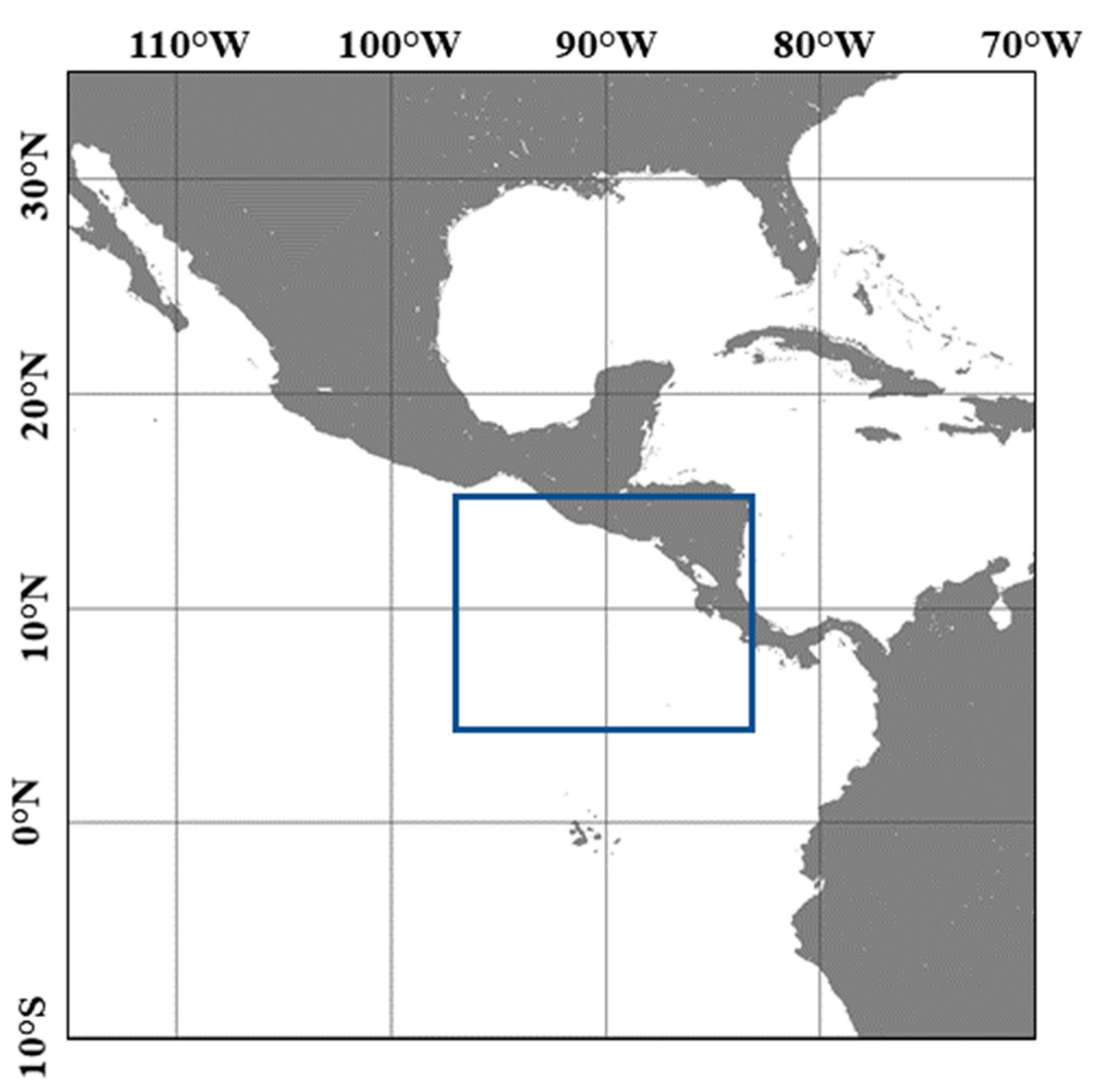
:1. Introduction
2. Data and Methods
2.1. VIIRS Satellite Ocean Color Products
2.2. SST and SSS Data
2.3. In Situ Data
3. Results
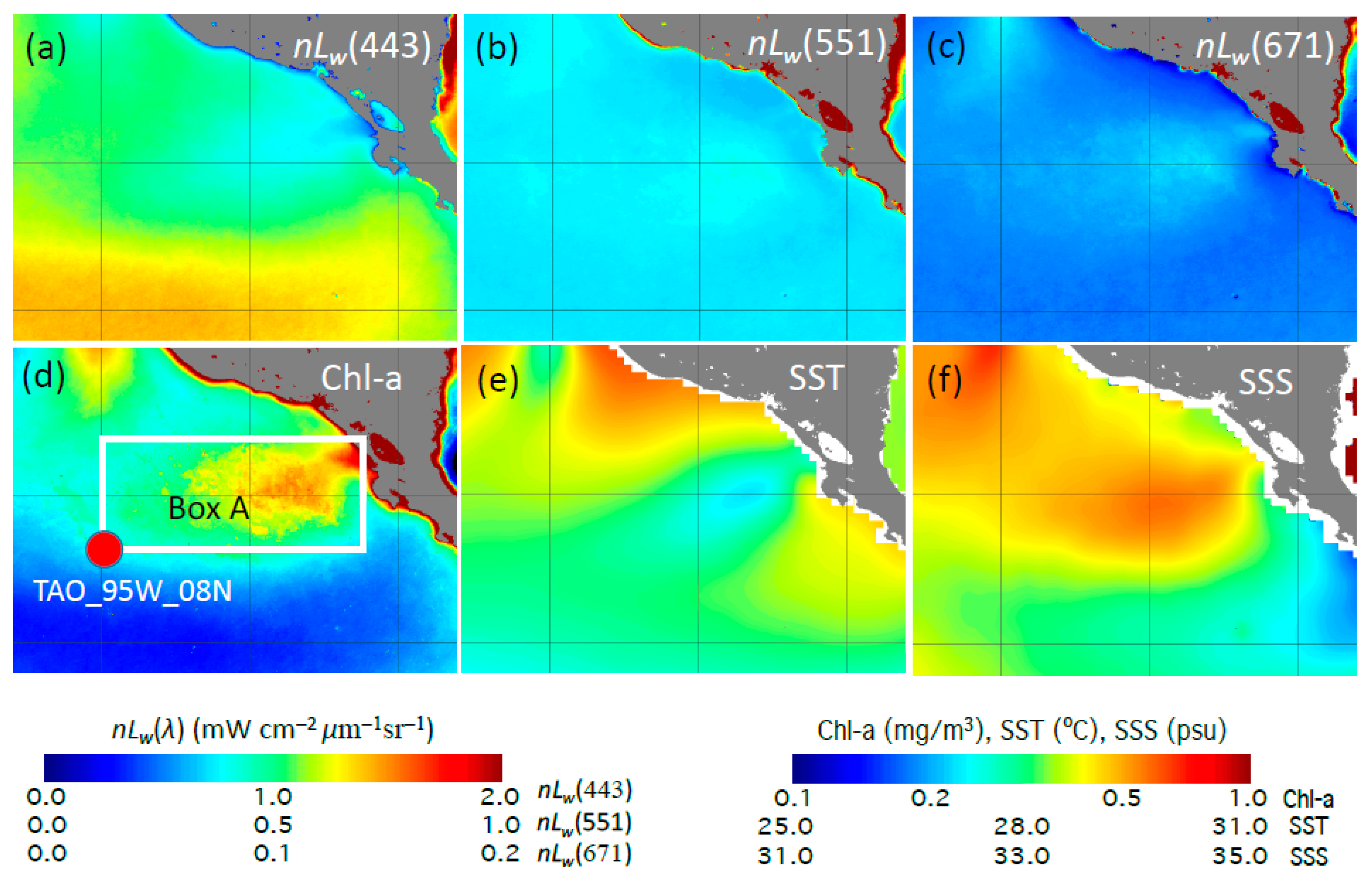
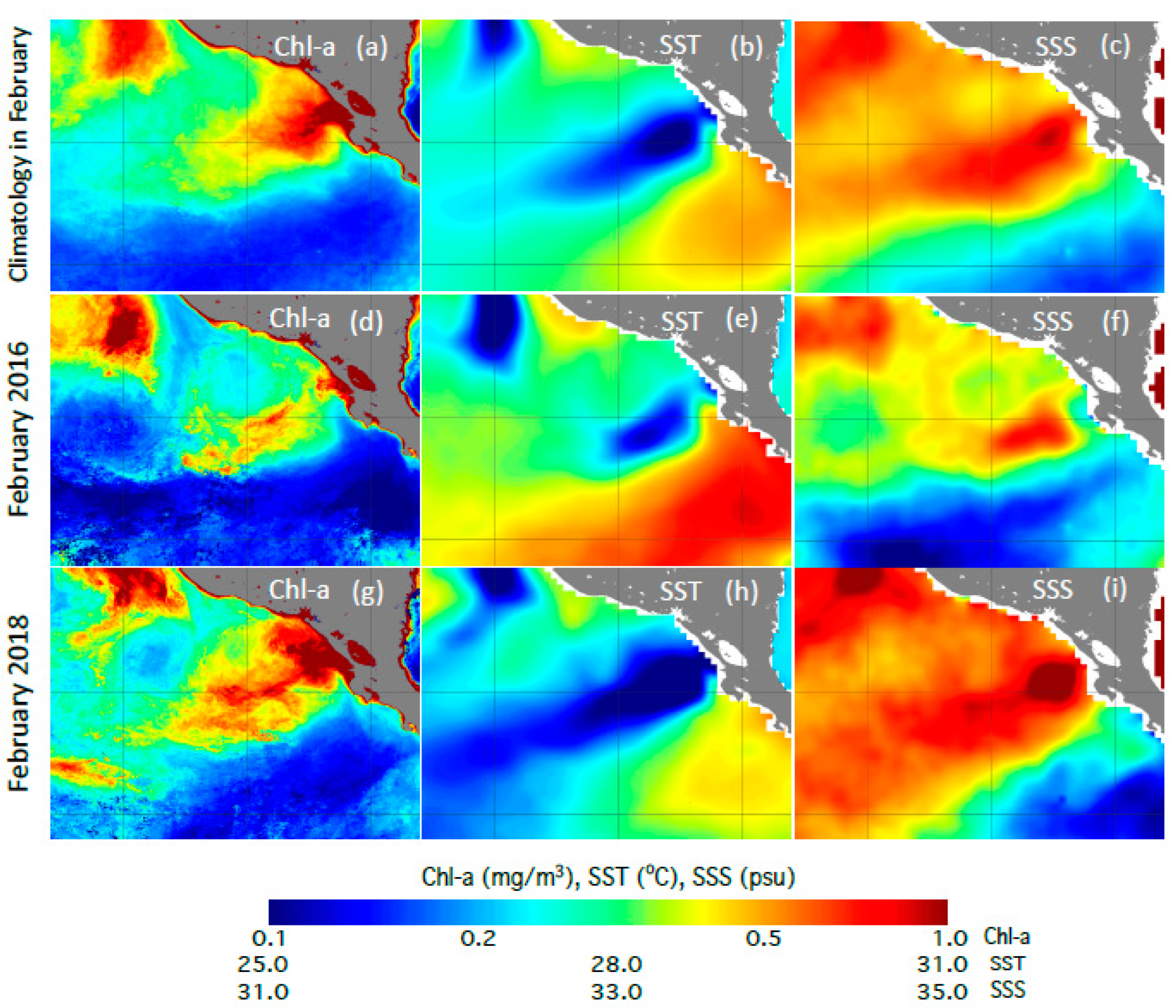
3.1. Climatology of nLw(λ), Chl-a, SST, and SSS
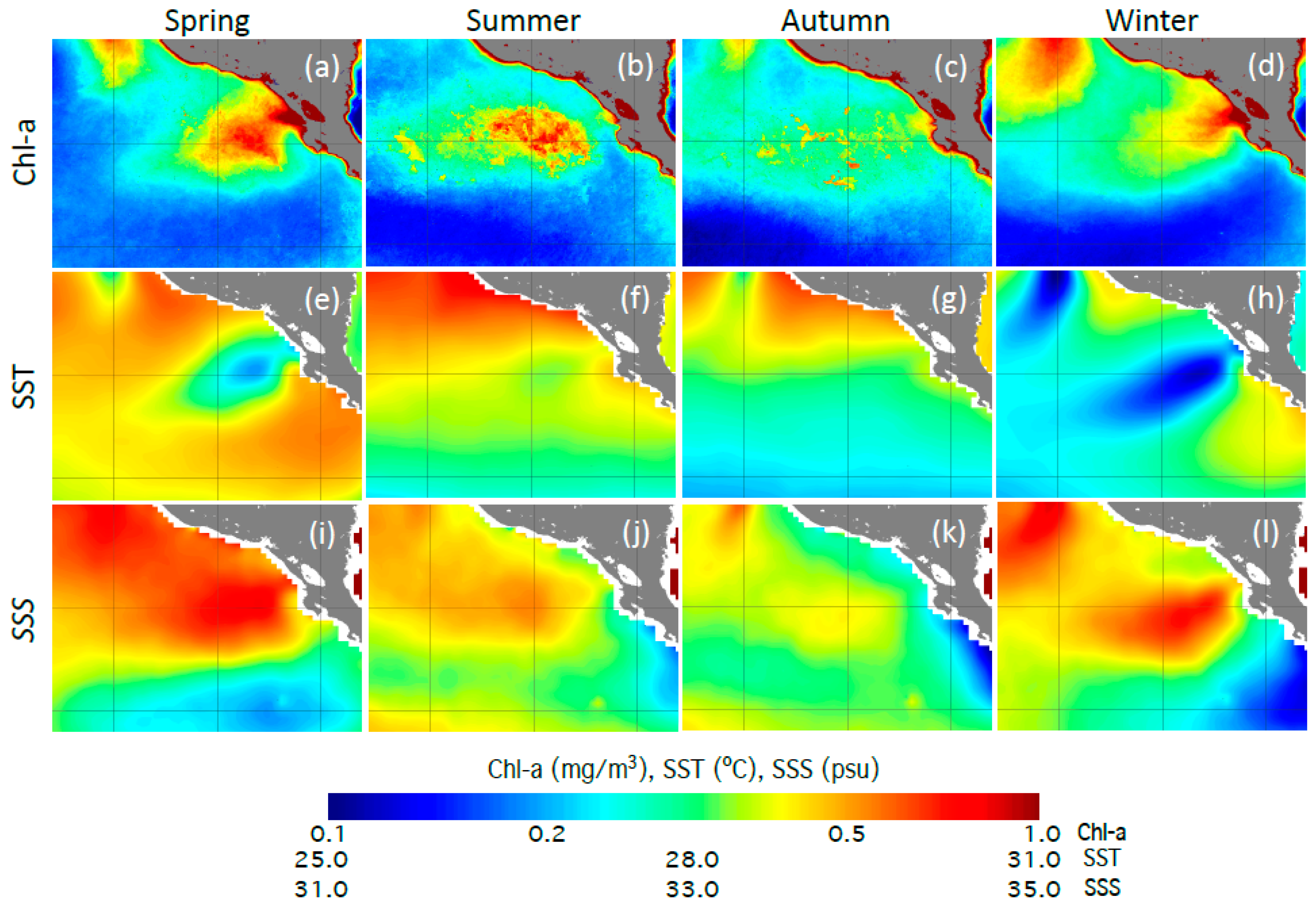
3.2. Seasonal Variability in nLw(λ), Chl-a, SST, and SSS
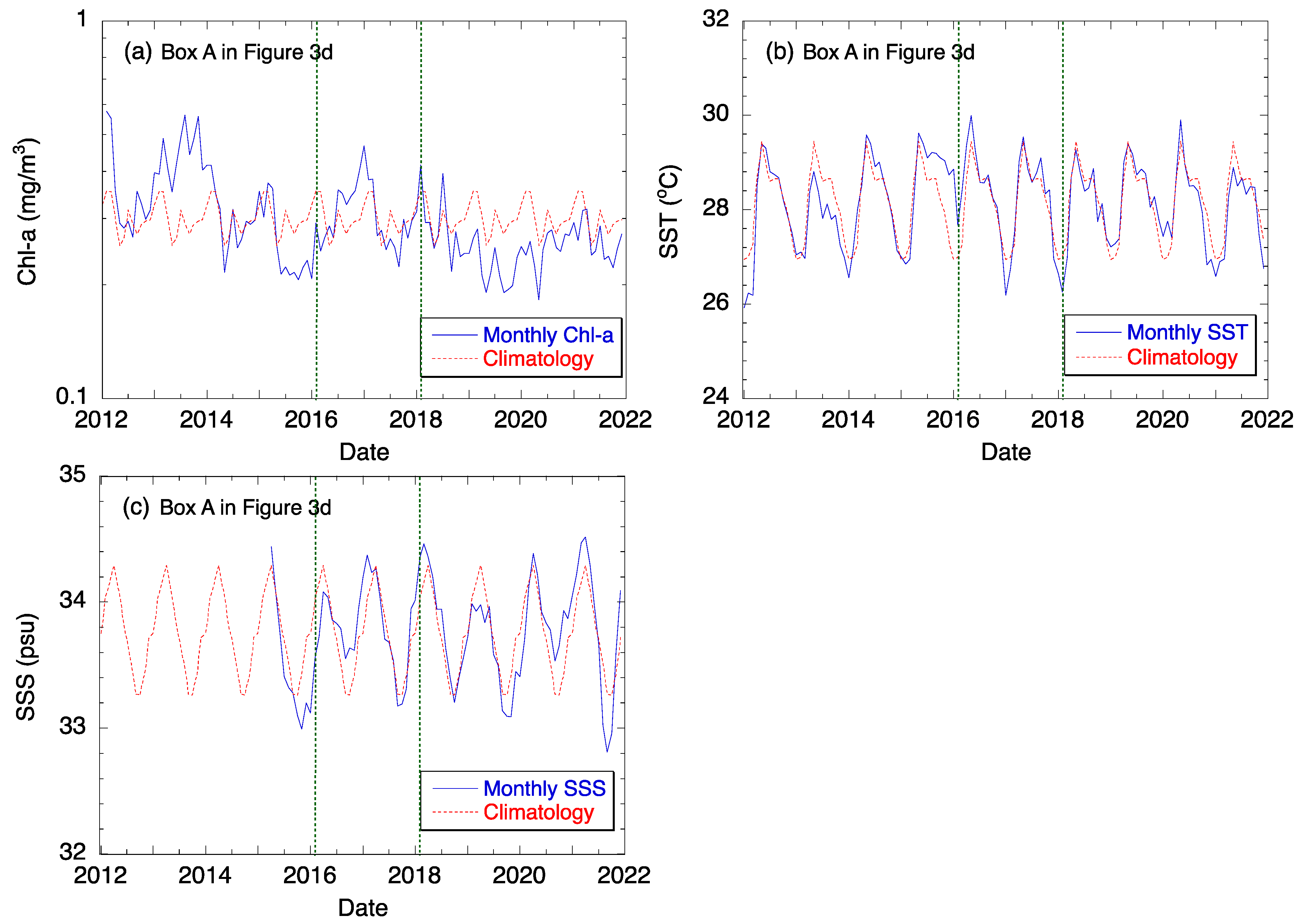
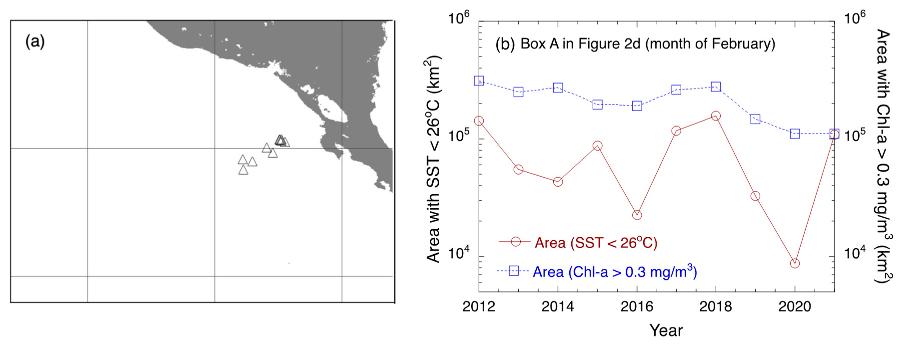
3.3. Interannual Variability in Chl-a, SST, and SSS
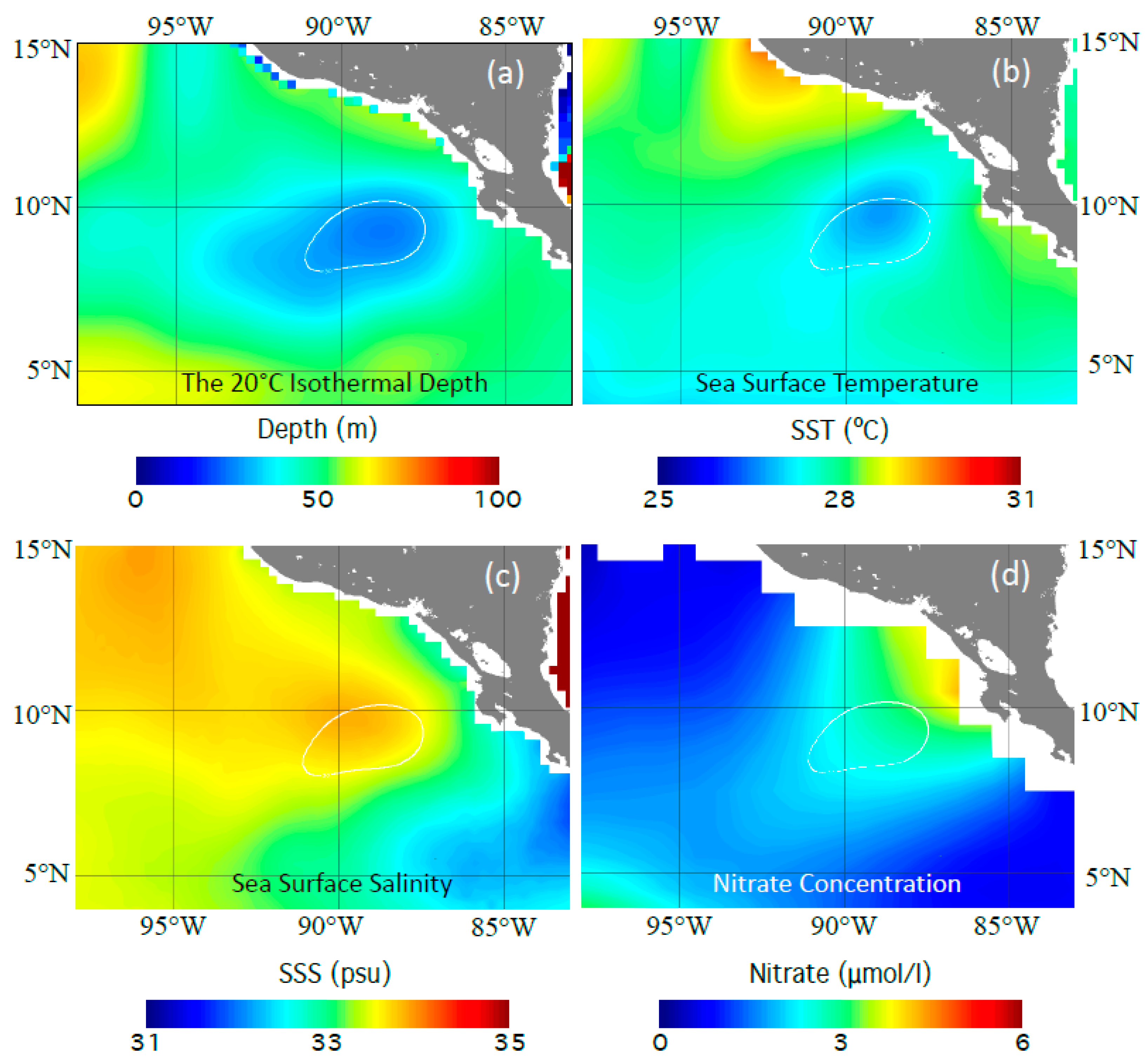
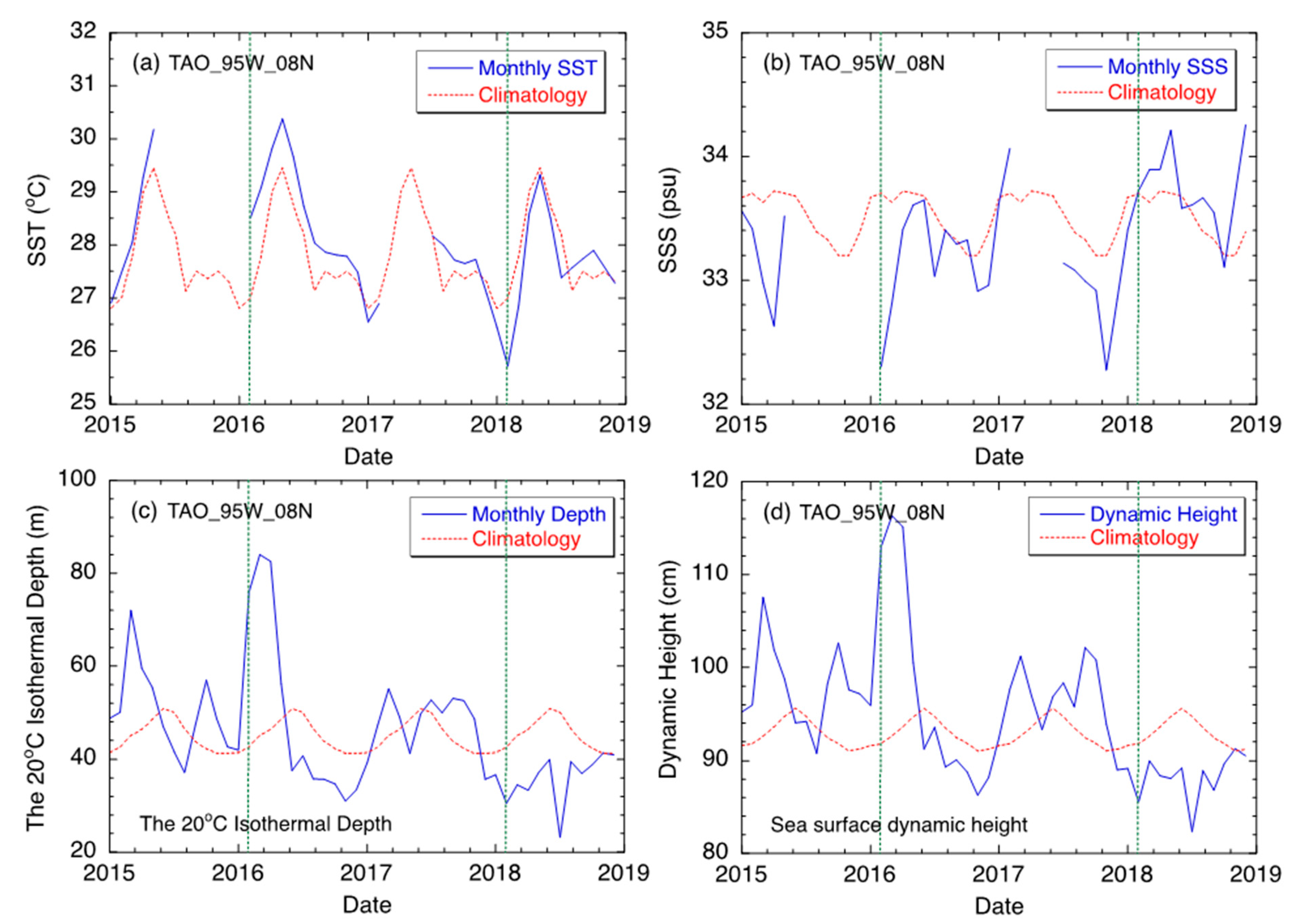
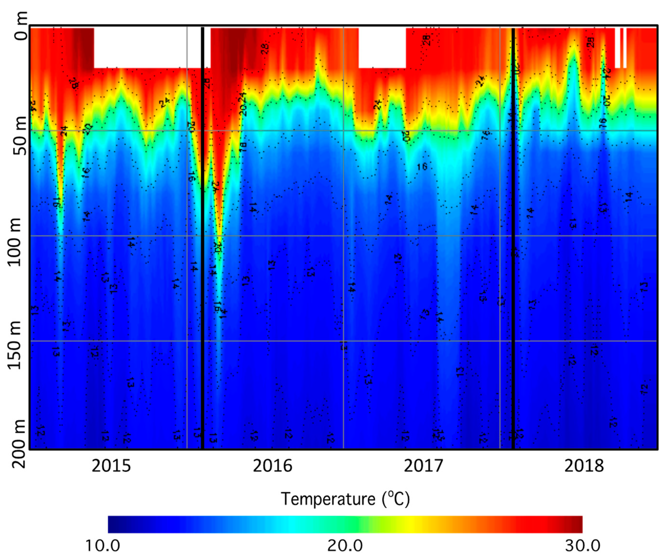
3.4. Subsurface Variability in the CRTD Region
4. Discussion
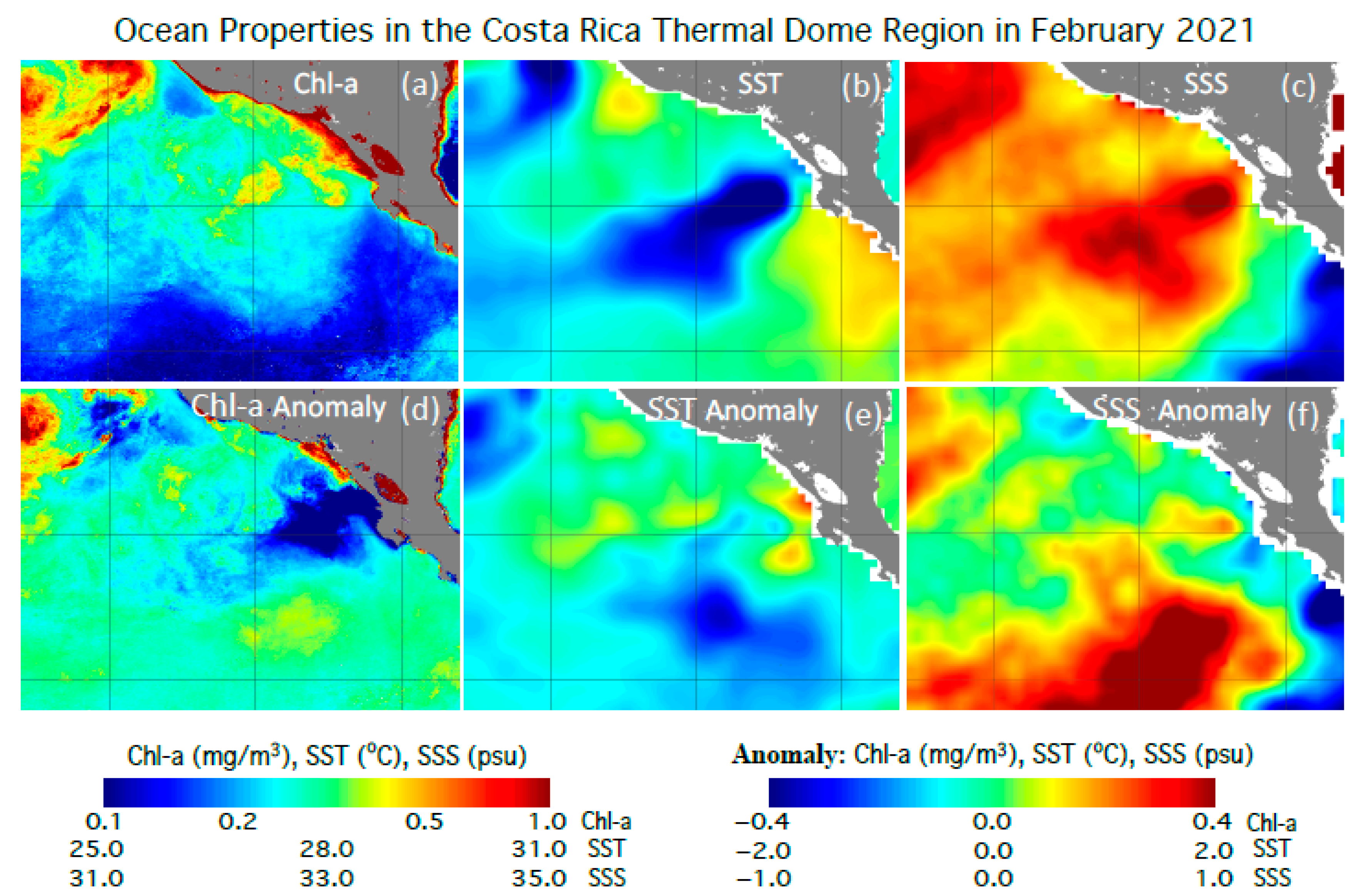
4.1. Linkage among Chl-a, SST, and SSS Features
4.2. ENSO Impact on Chl-a, SST, and SSS Features
5. Conclusions
Author Contributions
Funding
Data Availability Statement
Acknowledgments
Conflicts of Interest
References
- Cromwell, T. Thermocline topography, horizontal currents and “ridging” in the eastern tropical Pacific. Bull. Inter-Am. Trop. Tuna Comm. 1958, 111, 135–164. [Google Scholar]
- Wyrtki, K. Upwelling in the Costa Rica Dome. Fish. Bull. 1964, 63, 355–372. [Google Scholar]
- Fiedler, P.C. The annual cycle and biological effects of the Costa Rica Dome. Deep-Sea Res. Part I 2002, 49, 321–338. [Google Scholar] [CrossRef]
- Jimenez, J. The Costa Rica Thermic Dome; MarViva: Romsey, UK, 2017; p. 55. [Google Scholar]
- Wyrtki, K.; Kendall, R. Transports of the Pacific Equatorial Countercurrent. J. Geophys. Res. 1967, 72, 2073–2076. [Google Scholar] [CrossRef]
- McPhaden, M.J. Monthly period oscillations in the Pacific North Equatorial Countercurrent. J. Geophys. Res. Oceans 1996, 101, 6337–6359. [Google Scholar] [CrossRef]
- Zhao, J.; Li, Y.L.; Wang, F. Dynamical responses of the west Pacific North Equatorial Countercurrent (NECC) system to El Nino events. J. Geophys. Res. Oceans 2013, 118, 2828–2844. [Google Scholar] [CrossRef]
- Kessler, W.S. The circulation of the eastern tropical Pacific: A review. Prog. Oceanogr. 2006, 69, 181–217. [Google Scholar] [CrossRef]
- Schonau, M.C.; Rudnick, D.L. Glider observations of the North Equatorial Current in the western tropical Pacific. J. Geophys. Res. Oceans 2015, 120, 3586–3605. [Google Scholar] [CrossRef]
- Hofmann, E.E.; Busalacchi, A.J.; Obrien, J.J. Wind Generation of the Costa-Rica Dome. Science 1981, 214, 552–554. [Google Scholar] [CrossRef]
- Umatani, S.; Yamagata, T. Response of the Eastern Tropical Pacific to Meridional Migration of the Itcz—The Generation of the Costa-Rica Dome. J. Phys. Ocean. 1991, 21, 346–363. [Google Scholar] [CrossRef]
- Sasai, Y.; Sasaki, H.; Sasaoka, K.; Ishida, A.; Yamanaka, Y. Marine ecosystem simulation in the eastern tropical Pacific with a global eddy resolving coupled physical-biological model. Geophys. Res. Lett. 2007, 34, L23601. [Google Scholar] [CrossRef]
- Broenkow, W.W. The distribution of nutrients in the costa rica dome in the eastern tropical pacific ocean. Limnol. Oceanogr. 1965, 10, 40–52. [Google Scholar] [CrossRef]
- McClain, C.R.; Christian, J.R.; Signorini, S.R.; Lewis, M.R.; Asanuma, I.; Turk, D.; Dupouy-Douchement, C. Satellite ocean-color observations of the tropical Pacific Ocean. Deep-Sea Res. Part II 2002, 49, 2533–2560. [Google Scholar] [CrossRef]
- Fiedler, P.C.; Philbrick, V.; Chavez, F.P. Oceanic Upwelling and Productivity in the Eastern Tropical Pacific. Limnol. Oceanogr. 1991, 36, 1834–1850. [Google Scholar] [CrossRef]
- Sasai, Y.; Richards, K.J.; Ishida, A.; Sasaki, H. Spatial and temporal variabilities of the chlorophyll distribution in the northeastern tropical Pacific: The impact of physical processes on seasonal and interannual time scales. J. Mar. Syst. 2012, 96–97, 24–31. [Google Scholar] [CrossRef]
- Pennington, J.T.; Mahoney, K.L.; Kuwahara, V.S.; Kolber, D.D.; Calienes, R.; Chavez, F.P. Primary production in the eastern tropical Pacific: A review. Prog. Oceanogr. 2006, 69, 285–317. [Google Scholar] [CrossRef]
- Barber, R.T.; Chavez, F.P. Regulation of Primary Productivity Rate in the Equatorial Pacific. Limnol. Oceanogr. 1991, 36, 1803–1815. [Google Scholar] [CrossRef]
- Landry, M.R.; Selph, K.E.; Decima, M.; Gutierrez-Rodriguez, A.; Stukel, M.R.; Taylor, A.G.; Pasulka, A.L. Phytoplankton production and grazing balances in the Costa Rica Dome. J. Plankton Res. 2016, 38, 366–379. [Google Scholar] [CrossRef] [PubMed]
- Minas, H.J.; Minas, M. Net Community Production in High Nutrient-Low Chlorophyll Waters of the Tropical and Antarctic Oceans—Grazing Vs Iron Hypothesis. Ocean. Acta 1992, 15, 145–162. [Google Scholar]
- Fernandez-Alamo, M.A.; Farber-Lorda, J. Zooplankton and the oceanography of the eastern tropical Pacific: A review. Prog. Oceanogr. 2006, 69, 318–359. [Google Scholar] [CrossRef]
- Sameoto, D.; Guglielmo, L.; Lewis, M.K. Day Night Vertical-Distribution of Euphausiids in the Eastern Tropical Pacific. Mar. Biol. 1987, 96, 235–245. [Google Scholar] [CrossRef]
- Evseenko, S.A.; Shtaut, M.I. On the Species Composition and Distribution of Ichthyoplankton and Micronekton in the Costa Rica Domeand Adjacent Areas of the Tropical Eastern Pacific. J. Ichthyol. 2005, 45, 512–524. [Google Scholar]
- Joseph, J. The Tuna-Dolphin Controversy in the Eastern Pacific-Ocean—Biological, Economic, and Political Impacts. Ocean. Dev. Int. Law. 1994, 25, 1–30. [Google Scholar] [CrossRef]
- De Anda-Montanez, J.A.; Amador-Buenrostro, A.; Martinez-Aguilar, S.; Muhlia-Almazan, A. Spatial analysis of yellowfin tuna (Thunnus albacares) catch rate and its relation to El Nino and La Nina events in the eastern tropical Pacific. Deep-Sea Res. Part II 2004, 51, 575–586. [Google Scholar] [CrossRef]
- Behringer, D.W.; Ji, M.; Leetmaa, A. An improved coupled model for ENSO prediction and implications for ocean initialization. Part I: The Ocean Data Assimilation System. Mon. Weather. Rev. 1998, 126, 1013–1021. [Google Scholar] [CrossRef]
- Derber, J.; Rosati, A. A Global Oceanic Data Assimilation System. J. Phys. Ocean. 1989, 19, 1333–1347. [Google Scholar] [CrossRef]
- O’Neill, P.; Entekhabi, D.; Njoku, E.; Kellogg, K. The Nasa Soil Moisture Active Passive (Smap) Mission: Overview. In Proceedings of the 2010 Ieee International Geoscience and Remote Sensing Symposium, Honolulu, HI, USA, 25–30 July 2010; pp. 3236–3239. [Google Scholar] [CrossRef]
- Salomonson, V.V.; Barnes, W.L.; Maymon, P.W.; Montgomery, H.E.; Ostrow, H. Modis—Advanced Facility Instrument for Studies of the Earth as a System. IEEE Trans. Geosci. Remote Sens. 1989, 27, 145–153. [Google Scholar] [CrossRef]
- Esaias, W.E.; Abbott, M.R.; Barton, I.; Brown, O.B.; Campbell, J.W.; Carder, K.L.; Clark, D.K.; Evans, R.H.; Hoge, F.E.; Gordon, H.R.; et al. An overview of MODIS capabilities for ocean science observations. IEEE Trans. Geosci. Remote Sens. 1998, 36, 1250–1265. [Google Scholar] [CrossRef]
- Goldberg, M.D.; Kilcoyne, H.; Cikanek, H.; Mehta, A. Joint Polar Satellite System: The United States next generation civilian polar-orbiting environmental satellite system. J. Geophys. Res. Atmos. 2013, 118, 13463–13475. [Google Scholar] [CrossRef]
- Wang, M.; Liu, X.; Tan, L.; Jiang, L.; Son, S.; Shi, W.; Rausch, K.; Voss, K. Impacts of VIIRS SDR performance on ocean color products. J. Geophys. Res. Atmos. 2013, 118, 10347–10360. [Google Scholar] [CrossRef]
- Gordon, H.R.; Wang, M. Retrieval of Water-Leaving Radiance and Aerosol Optical-Thickness over the Oceans with Seawifs—A Preliminary Algorithm. Appl. Opt. 1994, 33, 443–452. [Google Scholar] [CrossRef] [PubMed]
- Wang, M.; Shi, W. The NIR-SWIR combined atmospheric correction approach for MODIS ocean color data processing. Opt. Expr. 2007, 15, 15722–15733. [Google Scholar] [CrossRef] [PubMed]
- Wang, M. Remote sensing of the ocean contributions from ultraviolet to near-infrared using the shortwave infrared bands: Simulations. Appl. Opt. 2007, 46, 1535–1547. [Google Scholar] [CrossRef]
- McClain, C.R.; Feldman, G.C.; Hooker, S.B. An overview of the SeaWiFS project and strategies for producing a climate research quality global ocean bio-optical time series. Deep-Sea Res. Part II 2004, 51, 5–42. [Google Scholar] [CrossRef]
- McClain, C.R. A Decade of Satellite Ocean Color Observations. Annu. Rev. Mar. Sci. 2009, 1, 19–42. [Google Scholar] [CrossRef] [PubMed]
- Clark, D.K.; Gordon, H.R.; Voss, K.J.; Ge, Y.; Broenkow, W.; Trees, C. Validation of atmospheric correction over the oceans. J. Geophys. Res-Atmos. 1997, 102, 17209–17217. [Google Scholar] [CrossRef]
- Wang, M.; Shi, W.; Jiang, L.; Voss, K. NIR- and SWIR-based on-orbit vicarious calibrations for satellite ocean color sensors. Opt. Expr. 2016, 24, 20437–20453. [Google Scholar] [CrossRef]
- Barnes, B.B.; Cannizzaro, J.P.; English, D.C.; Hu, C.M. Validation of VIIRS and MODIS reflectance data in coastal and oceanic waters: An assessment of methods. Remote Sens. Environ. 2019, 220, 110–123. [Google Scholar] [CrossRef]
- Mikelsons, K.; Wang, M.H.; Jiang, L.D. Statistical evaluation of satellite ocean color data retrievals. Remote Sens. Environ. 2020, 237, 111601. [Google Scholar] [CrossRef]
- Wang, M.; Shi, W.; Watanabe, W. Satellite-measured water properties in high altitude Lake Tahoe. Water Res. 2020, 178, 115839. [Google Scholar] [CrossRef]
- Hu, C.; Lee, Z.; Franz, B. Chlorophyll a algorithms for oligotrophic oceans: A novel approach based on three-band reflectance difference. J. Geophys. Res. Oceans 2012, 117, C01011. [Google Scholar] [CrossRef]
- Wang, M.; Son, S. VIIRS-derived chlorophyll-a using the ocean color index method. Remote Sens. Environ. 2016, 182, 141–149. [Google Scholar] [CrossRef]
- O’Reilly, J.E.; Maritorena, S.; Mitchell, B.G.; Siegel, D.A.; Carder, K.L.; Garver, S.A.; Kahru, M.; McClain, C. Ocean color chlorophyll algorithms for SeaWiFS. J. Geophys. Res. Oceans 1998, 103, 24937–24953. [Google Scholar] [CrossRef]
- O’Reilly, J.E.; Werdell, P.J. Chlorophyll algorithms for ocean color sensors-OC4, OC5 & OC6. Remote Sens. Environ. 2019, 229, 32–47. [Google Scholar] [CrossRef] [PubMed]
- Ravichandran, M.; Behringer, D.; Sivareddy, S.; Girishkumar, M.S.; Chacko, N.; Harikumar, R. Evaluation of the Global Ocean Data Assimilation System at INCOIS: The Tropical Indian Ocean. Ocean Model. 2013, 69, 123–135. [Google Scholar] [CrossRef]
- Behringer, D.W.; Xue, Y. Evaluation of the global ocean data assimilation system at NCEP: The Pacific Ocean. In Proceedings of the Eighth Symposium on Integrated Observing and Assimilation Systems for Atmosphere, Oceans, and Land Surface AMS 84th Annual Meeting, Seattle, WA, USA, 11–14 January 2004. [Google Scholar]
- Fore, A.G.; Yueh, S.H.; Tang, W.Q.; Stiles, B.W.; Hayashi, A.K. Combined Active/Passive Retrievals of Ocean Vector Wind and Sea Surface Salinity With SMAP. IEEE Trans. Geosci. Remote Sens. 2016, 54, 7396–7404. [Google Scholar] [CrossRef]
- Chan, S.K.; Bindlish, R.; O’Neill, P.E.; Njoku, E.; Jackson, T.; Colliander, A.; Chen, F.; Burgin, M.; Dunbar, S.; Piepmeier, J.; et al. Assessment of the SMAP Passive Soil Moisture Product. IEEE Trans. Geosci. Remote Sens. 2016, 54, 4994–5007. [Google Scholar] [CrossRef]
- Tang, W.Q.; Fore, A.; Yueh, S.; Lee, T.; Hayashi, A.; Sanchez-Franks, A.; Martinez, J.; King, B.; Baranowski, D. Validating SMAP SSS with in situ measurements. Remote Sens. Environ. 2017, 200, 326–340. [Google Scholar] [CrossRef]
- Mcphaden, M.J. The Tropical Atmosphere Ocean Array Is Completed. Bull. Am. Meteorol. Soc. 1995, 76, 739–741. [Google Scholar] [CrossRef]
- McPhaden, M.J.; Busalacchi, A.J.; Cheney, R.; Donguy, J.R.; Gage, K.S.; Halpern, D.; Ji, M.; Julian, P.; Meyers, G.; Mitchum, G.T.; et al. The tropical ocean global atmosphere observing system: A decade of progress. J. Geophys. Res. Oceans 1998, 103, 14169–14240. [Google Scholar] [CrossRef]
- Shi, W.; Wang, M. Phytoplankton biomass dynamics in the Arabian Sea from VIIRS observations. J. Mar. Syst. 2022, 227, 103670. [Google Scholar] [CrossRef]
- Garcia, H.E.; Weathers, K.W.; Paver, C.R.; Smolyar, I.; Boyer, T.P.; Locarnini, R.A.; Zweng, M.M.; Mishonov, A.V.; Baranova, O.K.; Seidov, D.; et al. World Ocean Atlas 2018. Vol. 4: Dissolved Inorganic Nutrients (Phosphate, Nitrate and Nitrate+Nitrite, Silicate); NOAA Atlas NESDIS 84; NOAA: Silver Spring, MD, USA, 2019; p. 35.
- Wolter, K. The Southern Oscillation in Surface Circulation and Climate over the Tropical Atlantic, Eastern Pacific, and Indian Oceans as Captured by Cluster-Analysis. J. Clim. Appl. Meteorol. 1987, 26, 540–558. [Google Scholar] [CrossRef]
- Wolter, K.; Timlin, M.S. El Nino/Southern Oscillation behaviour since 1871 as diagnosed in an extended multivariate ENSO index (MEI.ext). Int. J. Clim. 2011, 31, 1074–1087. [Google Scholar] [CrossRef]
- Kao, H.Y.; Yu, J.Y. Contrasting Eastern-Pacific and Central-Pacific Types of ENSO. J. Clim. 2009, 22, 615–632. [Google Scholar] [CrossRef]
- Yu, J.Y.; Kim, S.T. Identification of Central-Pacific and Eastern-Pacific types of ENSO in CMIP3 models. Geophys. Res.Lett. 2010, 37, L15705. [Google Scholar] [CrossRef]
- Jeng, H.; Ahn, J. A new method to classify ENSO events into eastern and central Pacific types. Int. J. Climatol. 2016, 37, 2193–2199. [Google Scholar] [CrossRef]


| Parameter | Feb. Clim. Mean | Feb. Clim. Median | Feb. 2016 Mean | Feb. 2016 Median | Feb. 2018 Mean | Feb. 2018 Median |
|---|---|---|---|---|---|---|
| Chl-a (mg/m3) | 0.441 | 0.364 | 0.322 | 0.291 | 0.490 | 0.417 |
| SST (°C) | 26.99 | 27.14 | 27.67 | 27.87 | 26.25 | 26.32 |
| SSS (psu) | 34.09 | 34.04 | 33.55 | 33.51 | 34.35 | 34.33 |
Disclaimer/Publisher’s Note: The statements, opinions and data contained in all publications are solely those of the individual author(s) and contributor(s) and not of MDPI and/or the editor(s). MDPI and/or the editor(s) disclaim responsibility for any injury to people or property resulting from any ideas, methods, instructions or products referred to in the content. |
© 2024 by the authors. Licensee MDPI, Basel, Switzerland. This article is an open access article distributed under the terms and conditions of the Creative Commons Attribution (CC BY) license (https://creativecommons.org/licenses/by/4.0/).
Share and Cite
Shi, W.; Wang, M. Ocean Variability in the Costa Rica Thermal Dome Region from 2012 to 2021. Remote Sens. 2024, 16, 1340. https://doi.org/10.3390/rs16081340
Shi W, Wang M. Ocean Variability in the Costa Rica Thermal Dome Region from 2012 to 2021. Remote Sensing. 2024; 16(8):1340. https://doi.org/10.3390/rs16081340
Chicago/Turabian StyleShi, Wei, and Menghua Wang. 2024. "Ocean Variability in the Costa Rica Thermal Dome Region from 2012 to 2021" Remote Sensing 16, no. 8: 1340. https://doi.org/10.3390/rs16081340