Shadow-Aware Point-Based Neural Radiance Fields for High-Resolution Remote Sensing Novel View Synthesis

Abstract

Novel view synthesis using neural radiance fields (NeRFs) for remote sensing images is important for various applications. Traditional methods often use implicit representations for modeling, which have slow rendering speeds and cannot directly obtain the structure of the 3D scene. Some studies have introduced explicit representations, such as point clouds and voxels, but this kind of method often produces holes when processing large-scale scenes from remote sensing images. In addition, NeRFs with explicit 3D expression are more susceptible to transient phenomena (shadows and dynamic objects) and even plane holes. In order to address these issues, we propose an improved method for synthesizing new views of remote sensing images based on Point-NeRF. Our main idea focuses on two aspects: filling in the spatial structure and reconstructing ray-marching rendering using shadow information. First, we introduce hole detection, conducting inverse projection to acquire candidate points that are adjusted during training to fill the holes. We also design incremental weights to reduce the probability of pruning the plane points. We introduce a geometrically consistent shadow model based on a point cloud to divide the radiance into albedo and irradiance, allowing the model to predict the albedo of each point, rather than directly predicting the radiance. Intuitively, our proposed method uses a sparse point cloud generated with traditional methods for initialization and then builds the dense radiance field. We evaluate our method on the LEVIR_NVS data set, demonstrating its superior performance compared to state-of-the-art methods. Overall, our work provides a promising approach for synthesizing new viewpoints of remote sensing images.

1. Introduction

Due to the ability to capture global features on a larger geographical scale, remote sensing images have advantages in the context of road extraction [1,2,3,4], urban planning [5], and object detection [6], whereas ground-based images often lack global information. With continuous advancements in aerial and satellite photography technologies, obtaining high-resolution remote sensing images has become much easier, allowing for the accurate identification of large structures, roads, rivers, and other man-made features, even for dynamic scenes. However, due to the limitation of the satellite camera’s angle and frequency, the image quantity for a specific area is often insufficient. Consequently, synthesizing novel views based on existing images has gradually become a mainstream data augmentation approach. Rendered images can help to enhance intelligence-gathering capabilities within target areas. Thus, the synthesis of remote sensing novel view images has attracted more and more attention.

Recently, NeRFs (neural radiance fields) [7] have been proposed to organically combine image-based 3D reconstruction and novel view synthesis. Unlike explicit 3D representation techniques, such as point clouds [8], volumes [9,10], or meshes [11], NeRFs employ an implicit representation method [12] to store 3D scenes within neural network weights. For each ray in an image, NeRF performs positional sampling and decodes the feature embedding, thus obtaining the radiance and volume density of each sampling point. Next, a ray-marching algorithm [13] is used to determine the color (RGB) and transparency of the specific pixel that the ray projects onto the image. With the color value as the ground truth, NeRF achieves simultaneous new view rendering and 3D structure optimization using radiance information. However, the implicit 3D representation lacks interpretability, and the efficiency of rendering ray by ray is too low for high-resolution remote sensing images. Moreover, the capture method of remote sensing images is different from standard close-range cameras, which creates larger distances between the targets and the camera. DoNeRFs [14] address this challenge by acquiring real-depth information and focusing on important samples around the object’s surface; however, obtaining accurate depth information is very difficult for remote sensing images. To this end, ImMPI [15] introduces implicit representation of 3D scenes using multi-plane images (MPIs) and performs novel view synthesis on remote sensing images. It also includes the LEVIR_NVS dataset, which comprises multi-scene and multi-view remote sensing data captured by drones. Despite this, NeRF and its variants (based on implicit 3D representations) still produce ineffective sampling in large blank areas [16], which not only reduces the overall performance efficiency but also causes rendering artifacts in some regions.

When compared to implicit expression, explicit 3D scene expression (e.g., point clouds and voxels) is more intuitive and is easier to combine with existing 3D application technologies [17,18,19]. Point-NeRF [20] first uses a point cloud as the skeleton of the neural radiation field to build a volume-rendering framework. Point-NeRF implements an effective algorithm to query adjacent points, based on which the point features located on rays can be calculated through adjacent point aggregation, with the radiance and transparency then decoded. Point-NeRF first uses MVSNet [21] to initialize the point cloud to fill the neural radiance field and then uses the VGG [22] model to extract feature vectors at each pixel position. During training, the model parameters, feature vectors, and confidence of each neural point are optimized synchronously. It is worth mentioning that Point-NeRF also introduces point cloud pruning and growing operations, dynamically encrypting neural clouds. Thus, Point-NeRF can process external point clouds, such as the photogrammetry point clouds generated by COLMAP [23].

However, directly applying Point-NeRF to the tasks of novel view synthesis from remote sensing images is challenging. At larger geographic scales, the original point cloud settings make it difficult to describe the whole scene and may result in large holes in the reconstruction results, which are mainly distributed in planar areas (such as straight roads and roofs), as shown in Figure 1. We believe that there are two main reasons for this: (1) the spatial density of the flat area is relatively low, and (2) the homogenization of a flat texture leads to poor optimization effects based on color values, causing the points on the plane to have low confidence and are, therefore, easily merged by pruning. We have also observed that these holes are mainly concentrated on buildings and roads in urban areas, whereas the quality of the mountains is quite good (as is shown in Figure 2). Thus, point cloud-based NeRF may be better at depicting continuous terrain rather than rapidly changing urban landscapes, which requires more structural prior knowledge and processing. On the other hand, Point-NeRF finds it difficult to render shadows that are closely related to 3D structures (examples in Figure 3), which inevitably results in the unpredictability of a scene.

Some studies have utilized NeRF to reconstruct digital surface models (DSMs) from remote sensing images, mainly focusing on the consideration of shadows. S-NeRF [24] reconsiders the radiance and rewrites it as the product of the albedo and irradiance, instead of directly estimating the whole radiance, as per the original NeRF. The albedo only relates to the location of the points and the scene information stored in the model, which is generated by an additional layer after the density network. Irradiance is a weighted sum of direct light from the sun and ambient light from the sky, both calculated by special modules based on solar direction. S-NeRF provides the basic idea for processing shadows—that is, splitting the original radiance and modeling the solar rays—based on the assumption that the difference between the location of the shadow and other locations is whether it can receive sunlight. Based on S-NeRF, Sat-NeRF [25] introduces an embedding vector to describe the characteristics of transient objects that cannot be captured by changes in illumination between different image frames. It also incorporates an uncertainty output to indicate whether a pixel belongs to a transient object. This approach partially decouples the features of shadows and transient objects. The iterative version, EO-NeRF [26], makes more intuitive use of the relationship between the solar ray and the spatial structure. It queries the position of the surface point through the camera ray and then determines whether the point is in the shadow region according to the radiance transmittance of the last term from the solar direction. Eo-NeRF [26] completely separates shadows and transient objects and adds two new learnable affine transform feature-embedding vectors to characterize the structural differences between images in different phases. This provides a new idea for our research.

Based on the above research, we adopt three methods to improve the current shortcomings of Point-NeRF. First, we utilize COLMAP to initialize the point cloud structure [23] using an existing projection matrix to obtain an initial 3D point cloud, instead of using the built-in MVSNet [21], which is then fed into the main model for optimization. In order to address the holes, we propose a new neural point-growing method, which is shown in Figure 4. Our main idea focuses on two aspects: filling in the spatial structure and reconstructing the ray-marching rendering using shadow information. First, we introduce hole detection and conduct inverse projection to acquire the candidate points that are adjusted during training to fill the holes. These 3D points are located in the light made up of the void point and the optical center, which will gradually converge to the correct position during training. We also design incremental weights to reduce the probability of pruning the plane points. Then, we introduce a geometrically consistent shadow model based on a point cloud to divide the radiance into albedo and irradiance according to the shadow information, allowing the model to decode more shadow-aware features. The neural point cloud is continuously optimized. After performing the above steps, we obtain an encrypted point cloud. Due to the introduction of shadow factors, we name the proposed method “shadow-aware Point-NeRF” (SA-Point-NeRF). Our method effectively compensates for the shortcomings of Point-NeRF, and experiments conducted on the LEVIR_NVS data set demonstrate the superiority of the proposed method over other state-of-the-art methods.

The contributions of this work can be summarized as follows:

• To the best of our knowledge, we are the first to apply Point-NeRF to the novel view synthesis of remote sensing images.
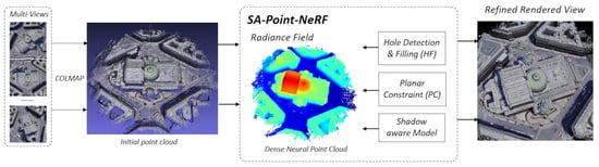
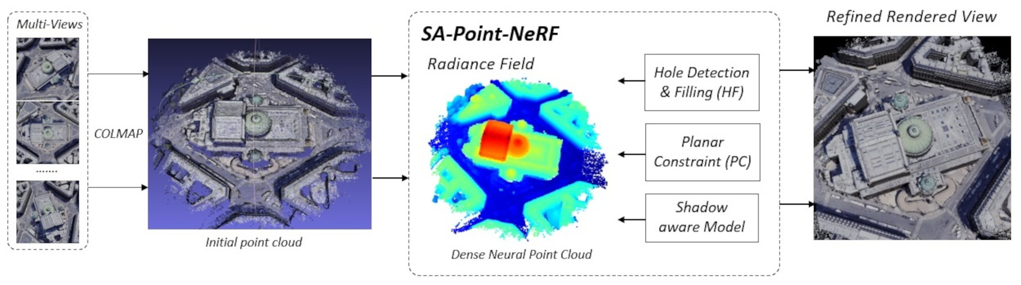
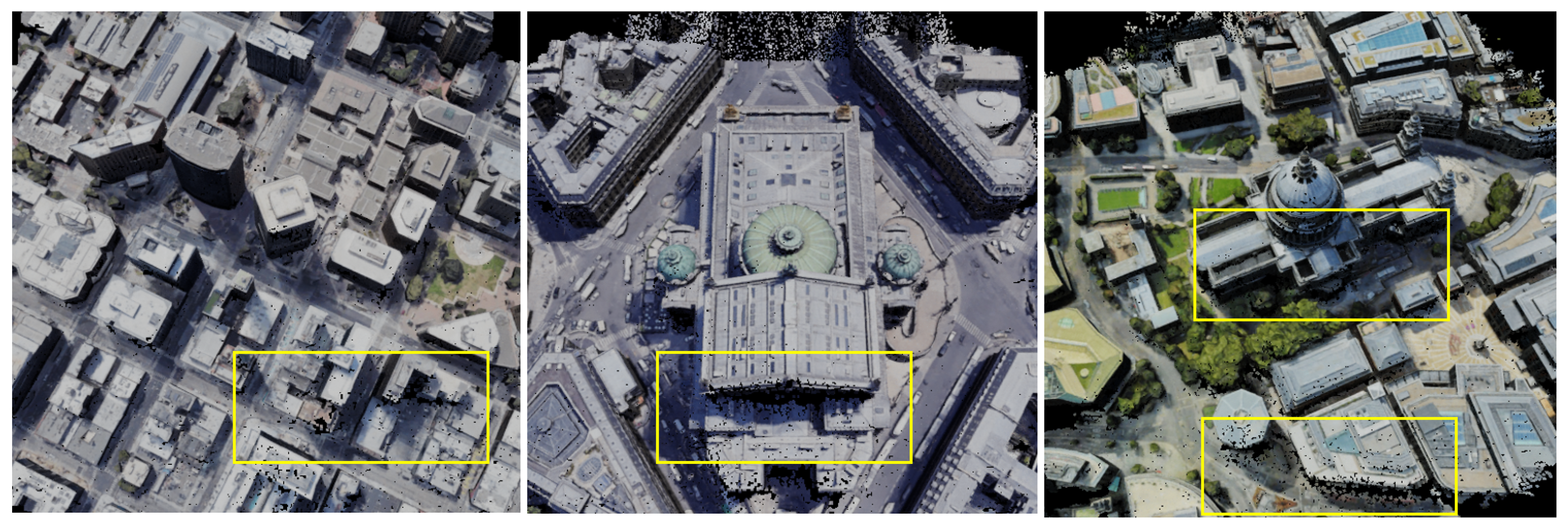
• We propose a new neural point-growing method, which detects holes in the rendered image and calculates some alternative 3D points through inverse projection. This method can effectively make up for the plane points being pruned by mistake.
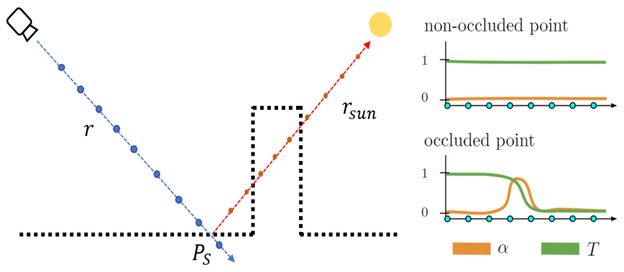
• We design a shadow model based on point cloud geometric consistency to deal with the holes in the shadow areas, which is useful for the perception of shadows.
• Our method was tested on the LEVIR_NVS data set and performed better than state-of-the-art methods.

2. Method

2.1. Preliminary

2.1.1. Neural Radiance Field

The original neural radiance field (NeRF) [7] is essentially a continuous function, $\mathcal{F}$, that stores the geometric structure and appearance of a 3D scene. In the simplest form, NeRF takes a set of 3D coordinates, $\mathbf{x}$, as input, and optionally, an appended view direction, $\mathbf{d}$, to predict the RGB color, $\mathbf{c}$, and a non-negative scalar volume density, $\sigma$, from that viewing angle, $\mathbf{d}$, which can be formulated as

$$\mathcal{F}:(\mathbf{x},\mathbf{d})\mapsto (\sigma ,\mathbf{c})$$

(1)

When training, NeRF takes the input view image and camera poses to encode Equation (1). Specifically, in each view, the origin of the camera light, $\mathbf{o}$, and pixel points constitute a ray, $\mathbf{r}$, and a multi-layer perceptron (MLP) estimates the state of each point in the ray, summing them to obtain the final color value, $\mathbf{c}\left(\mathbf{r}\right)$. Each ray, $\mathbf{r}$, can be represented as $\mathbf{r}\left(t\right)=\mathbf{o}+t\left(\mathbf{d}\right)$:

$$\mathbf{c}\left(\mathbf{r}\right)=\sum _{i=1}^N{T}_i{\alpha }_i{\mathbf{c}}_i$$

(2)

The rendered color, $\mathbf{c}\left(\mathbf{r}\right)$, is obtained by aggregating the states of the entire ray. Each ray is discretized into N 3D points, and each 3D point, ${\mathbf{x}}_i$, is moved by a certain step between the near boundary, $t_n$, and the far boundary, $t_f$, linearly, according to the formula ${\mathbf{x}}_i=\mathbf{o}+t_i\left(\mathbf{d}\right)$. The contribution of each point to $\mathbf{c}\left(\mathbf{r}\right)$ is determined by the opacity, ${\alpha }_i$, and transmittance, $T_i$.

$$\begin{array}{ccc}{\alpha }_i=1-exp(-{\sigma }_i{\delta }_i)& \mathrm{and}& T_i={\displaystyle \prod _{j=1}^{i-1}}(1-{\alpha }_j)\end{array}$$

(3)

where ${\delta }_i=t_{i+1}-t_i$ is the distance between adjacent samples. All these factors are taken in the interval $[0,1]$ and only rely on the volume density, $\sigma$. The opacity, $\alpha$, will increase with $\sigma$, and it denotes the probability that ${\mathbf{x}}_i$ belongs to a non-transparent surface. The transmittance, $T_i$, represents the probability of the ray reaching ${\mathbf{x}}_i$ without hitting an obstruction. Thus, the depth, $d\left(\mathbf{r}\right)$, can be calculated in a similar way as in Equation (2).

$$d\left(\mathbf{r}\right)=\sum _{i=1}^N{T}_i{\alpha }_i{t}_i$$

(4)

In the NeRF model, the MLP is responsible for estimating the most difficult volume density, $\sigma$, and the radiance, ${\mathbf{c}}_i$, of ${\mathbf{x}}_i$; thus, the RGB value, $\mathbf{c}\left(\mathbf{r}\right)$, can be calculated using the ray-marching algorithm described above. Then, the model is optimized by calculating the error between the rendered color, $\mathbf{c}\left(\mathbf{r}\right)$, and the ground image pixel color, ${\mathbf{c}}_{GT}\left(\mathbf{r}\right)$:

$$\sum _{\mathbf{r}\in \mathcal{R}}{∥\mathbf{c}\left(\mathbf{r}\right)-{\mathbf{c}}_{GT}\left(\mathbf{r}\right)∥}_2^2$$

(5)

where $\mathcal{R}$ is a batch of randomly selected rays during training.

2.1.2. Point-Based Neural Radiance Field

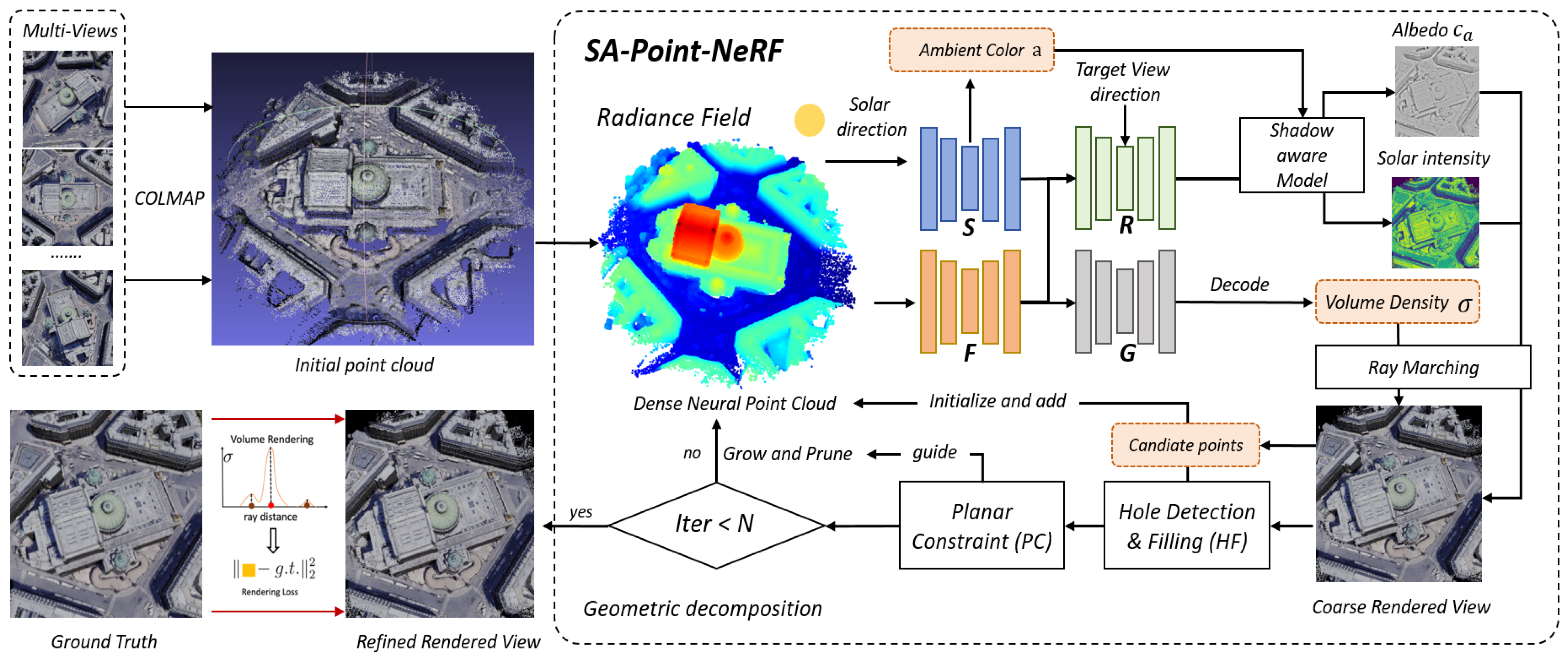
The radiation field used by NeRF is implicitly included in the MLP model, whereas Point-NeRF [20] uses a point cloud that includes M neural points as the skeleton. In this explicit representation, each point, ${\mathbf{x}}_j$, is assigned a neural embedding, $f_j$, and a confidence, ${\gamma }_j$, which are used to encode the radiation information and determine whether it is near the surface. The radiance field based on the neural point cloud can be expressed as

$$P=\left\{(p_j,f_j,{\gamma }_j)|j=1,...,M\right\}$$

(6)

As the radiance field is discretized, Point-NeRF aggregates the features of K neighborhood points when estimating the volume density, $\sigma$, of a point, x, and the view-independent radiance, r.

$$(\sigma ,r)=PointNeRF(x,d,p_1,f_1,{\gamma }_1,...p_K,f_K,{\gamma }_K)$$

(7)

Specifically, Point-NeRF first uses an MLP model, F, to encode the relationship between the existing neighbor points, $p_k|i=1,2,...K$, and the position, x, to be solved, generating relative features, $f_{i,x}$.

$$f_{k,x}=F(f_k,x-p_k)$$

(8)

Then, the view-dependent radiance at x is solved by another MLP, R, after the inverse distance-weighted aggregation of the relative neighborhood features:

$$r=R(f_x,d)$$

(9)

$$\begin{array}{ccc}{f}_x={\displaystyle \sum _k}{\gamma }_k\frac{{\omega }_k}{\sum {\omega }_k}{f}_{k,x}& \mathrm{and}& {\omega }_k=\frac{1}{∥p_k-x∥}\end{array}$$

(10)

For the volume density, $\sigma$, Point-NeRF first uses a new model, G, to directly calculate the density, ${\sigma }_k$, of each neighbor point according to $f_{k,x}$. Then, it obtains the aggregated $\sigma$ using inverse distance-weighted summation.

$${\sigma }_i=G\left(f_{k,x}\right)$$

(11)

$$\begin{array}{cc}\sigma ={\displaystyle \sum _k}{\sigma }_k{\gamma }_k\frac{{\omega }_k}{\sum {\omega }_k},& {\omega }_k=\frac{1}{∥p_k-x∥}\end{array}$$

(12)

Here, ${\gamma }_k$ adjusts the probability that the neural points are located on the surface; thus, the model can better converge to the real scene structure.

2.2. Overview

2.2.1. Main Workflow

We first define the outputs of our method. Then, we introduce the hole detection and filling method, which searches for points (i.e., black pixels) that are not rendered by any light on the generated image. Possible alternative points are then found using inverse projection. We initialize these points with feature embedding and put them into the neural point cloud for training. In this process, in order to reduce the unreasonable pruning of planar points, we introduce incremental weights to guide the regression of the volume density. Finally, we introduce a structural consistency shadow model based on a point cloud, which splits the radiance of Point-NeRF into albedo and irradiance regression, guiding volume rendering by judging whether a point is in a shadow. Thus, the model can produce shadow-aware features and reduce the rendering holes in shadow areas.

2.2.2. Module Function

Due to the discrete expression of radiance fields, the modules in Point-NeRF focus on aggregating neighborhood features instead of facing the whole ray. Therefore, taking the 3D point x as input, Point-NeRF first queries the neighborhood points from the point cloud to obtain the adjacent features, $f_1,f_2,\dots f_K$. Then, using the feature encoding module, $\mathbf{F}$ (MLP $\mathbf{F}$ in Figure 4), it completes the calculation of the relative features, $f_{1,x},f_{2,x},\dots f_{K,x}$, between x and these points. Then, the relative features and view direction, $\mathbf{d}$, are input into $\mathbf{R}$ (MLP $\mathbf{R}$ in Figure 4) to regress the albedo, ${\mathbf{c}}_{\mathbf{a}}$, as ${\mathbf{c}}_{\mathbf{a}}$ is view-dependent. The calculation of the volume density, $\sigma$, requires $\mathbf{G}$ (MLP $\mathbf{G}$ in Figure 4) to apply all the relative features. Finally, the ambient color is calculated by $\mathbf{S}$ (MLP $\mathbf{S}$ in Figure 4) from the perspective of the solar direction, ${\mathbf{d}}_{sun}$. The ambient color, albedo, and volume density all eventually contribute to the ray color, according to the ray-marching algorithm.

2.3. Problem Definition

The expanded neural radiance field of SA-Point-NeRF $P^s$ is

$$P^s=\left\{(p_j,f_j,{\gamma }_j,{\delta }_j,{\mathbf{c}}_j^a)|j=1,\dots ,M\right\}$$

(13)

Here, we expand the definition of the surface confidence, $\gamma$, in Point-NeRF to describe the structural information in more detail by adding a parameter, $\delta$. During training, $\delta$ determines whether the current point is on a plane, and this is calculated using the point density, $\sigma$.

Based on the above, the outputs of SA-Point-NeRF can be expressed as

$$\mathcal{F}:(\mathbf{x},{\mathbf{d}}_{sun},\mathbf{d},{\left\{{\mathbf{x}}_k\right\}}_{k=1}^K)\mapsto (\sigma ,{\mathbf{c}}_{\mathbf{a}},\mathbf{a},\gamma ,\delta )$$

(14)

The inputs of Equation (14) include the 3D point coordinates, $\mathbf{x}$; solar direction vector, ${\mathbf{d}}_{sun}$; current view direction, $\mathbf{d}$; and neighborhood points, ${\left\{{\mathbf{x}}_k\right\}}_{k=1}^K$. The outputs are as follows:

• $\sigma$: Volume density at location $\mathbf{x}$;
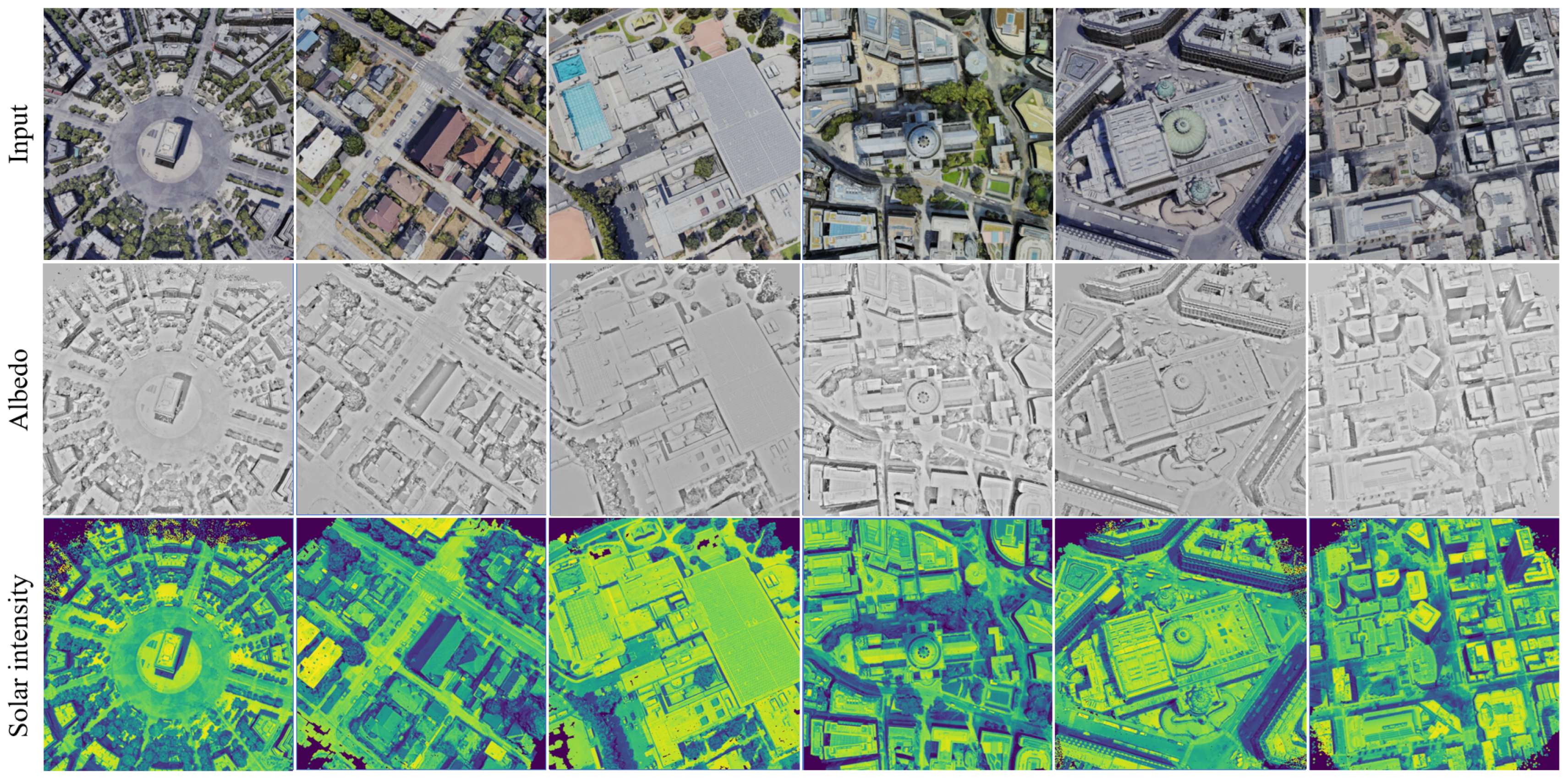
• ${\mathbf{c}}_{\mathbf{a}}$: Albedo RGB vector, only related to the spatial coordinate, $\mathbf{x}$;
• $\mathbf{a}$: Ambient color of the sky according to the solar direction, ${\mathbf{d}}_{sun}$;
• $\gamma$: Confidence of whether the point is near the surface;
• $\delta$: Confidence of whether the point belongs to a plane.

SA-Point-NeRF uses the output to render the color, $\mathbf{c}\left(\mathbf{r}\right)$, of a ray, $\mathbf{r}$, as follows:

$$\mathbf{c}\left(\mathbf{r}\right)=l\left(\mathbf{r}\right)\sum _{i=1}^N{T}_i{\alpha }_i{\mathbf{c}}_{\mathbf{a}}$$

(15)

where $l\left(\mathbf{r}\right)$ denotes the total irradiance and is defined as $l\left(\mathbf{r}\right)=s\left(\mathbf{r}\right)+(1-s(\mathbf{r}\left)\right)\mathbf{a}$, with $s\left(\mathbf{r}\right)$ defined in Equation (19).

2.4. Hole Detection and Filling

During training, we also introduce hole detection to find the corresponding candidate 3D coordinates. We only need to find the black pixels in the rendered image, $I_r$; that is, $\left\{(u,v)|I_{(u,v)}^r=(0,0,0)\right\}$. The pixel coordinates in the holes are denoted as ${[u,v,1]}^T$, the intrinsic matrix is denoted as $\mathbf{K}$, the rotation matrix is denoted as $\mathbf{R}$, the corresponding world coordinate is denoted as ${[X_w,Y_w,Z_w]}^T$, and the depth is denoted as z. Using these, we can build the inverse projection:

$$\left[\begin{array}{c}{X}_w\\ Y_w\\ Z_w\end{array}\right]={\mathbf{R}}^{-1}{\mathbf{K}}^{-1}z\left[\begin{array}{c}u\\ v\\ 1\end{array}\right]-{\mathbf{R}}^{-1}T$$

(16)

However, the depth cannot be determined using Equation (16). Thus, we chose the average depth, z, of the current point cloud to be $Z_w$, such that $X_w$ and $Y_w$ can be calculated. Although these points may not be on the surface, they are still located on the ray with holes, satisfying the projection equation. During the continuous optimization carried out by Point-NeRF, these points are gradually adjusted to the appropriate position.

2.5. Incremental Weight of Planar Information

We added the parameter $\delta$, indicating the probability of the point being on a plane. Unlike the original surface confidence, $\gamma$, which is independent, $\delta$ is obtained by aggregating neighborhood information because the planar point should share the relationship between neighborhood points. Specifically, when we use F to encode the features, we also make it judge whether the point has common conditions to become a plane point among the neighborhood points. That is, F outputs both the relative features, $f_{k,x}$, and planar confidence, ${\delta }_{k,x}$.

$$f_{k,x},{\delta }_{k,x}=F(f_k,{\delta }_k,x-p_k)$$

(17)

Then, the surface confidence, $\gamma$, and planar confidence, $\delta$, are used in the volume density regression. We consider that if the current point is on the surface, $\gamma +\delta$ will contribute more weight to the volume density, $\sigma$, and then the model will pay more attention to such a point, reducing the probability of pruning.

$$\sigma =\sum _k{\sigma }_k({\gamma }_k+{\delta }_k)\frac{{\omega }_i}{\sum {\omega }_i}$$

(18)

2.6. Structural Consistency Shadow Model

We introduce a sunlight model and a sky ambient color model to determine whether a point is in a shadow. Instead of directly estimating the radiance of x, we decomposed it into albedo and irradiance items. For this purpose, we added an albedo component, ${\mathbf{c}}_a$, to each neural point, $x_j$, which is decoded during per-point processing in Equation (8). Then, we decomposed the irradiance into direct solar radiance and sky ambient color, $\mathbf{a}$. The direct solar radiance, ${\mathbf{r}}_{sun}$, is calculated based on a point cloud-based structural consistency method, and the ambient color values are computed by a specialized model according to the solar direction, ${\mathbf{d}}_{sun}$. Considering that both the direct solar ray, ${\mathbf{r}}_{sun}$, and ambient colors, $\mathbf{a}$, affect the entire scene, we conducted the process only in the ray-marching algorithm, instead of embedding it into per-point attribution. As shown in Figure 5, we adopted the idea of the structural consistency shadow model in EO-NeRF, where the transmittance, T, of the last point in the solar ray, ${\mathbf{r}}_{sun}$, represents the shadow condition of the surface point, $P_s$. Unlike EO-NeRF, in our research, the surface is characterized using a discrete point cloud method, and the model automatically aggregates the features of neighboring points to generate the attribution. We can determine the surface point, $x_s$, using Equation (4) along the view direction, $\mathbf{d}$, and then place the point in the solar direction, ${\mathbf{d}}_{sun}$. Similarly, the transmittance, T, of this point can be calculated using Equation (3). If the transmittance is 0, it means that the point in the solar ray, ${\mathbf{r}}_{sun}$, is already occluded (i.e., the shadow area). If not, it means that the solar ray can reach its current position. For simplicity, we do not need to consider the changes in transient objects in our study without setting any transient object parameters. We denote the step of the surface point as $t_N$, and the irradiance, $s\left(\mathbf{r}\right)$, is defined as

$$s\left(\mathbf{r}\right)=T\left({\mathbf{r}}_{sun}\left(t_N\right)\right)=\prod _{i=1}^{N-1}(1-{\alpha }_i^{sun})$$

(19)

Meanwhile, the radiance decoder, R, in the original Point-NeRF also changes to predict the view-dependent albedo vector, ${\mathbf{c}}_{\mathbf{a}}$, which is formulated as

$${\mathbf{c}}_{\mathbf{a}}=R(f_x,d)$$

(20)

2.7. Loss Function

SA-Point-NeRF mainly uses three loss functions for optimization. The core loss function is still the radiance regression, ${\mathcal{L}}_{render}$, described by Equation (5). As our method only alters the calculation of the radiation but still outputs the rendered image, Equation (5) does not need to be modified. As we do not process transient objects, we continue to use the loss functions of Point-NeRF, including the rendering loss between the rendered color and image pixel and the sparse loss of surface confidence. In order to enhance the effect of planar confidence, we also designed sparse loss following the processing method of $\gamma$ in Point-NeRF:

$${\mathcal{L}}_{sparse}^{\delta }=\frac{1}{\left|\delta \right|}\sum _{{\delta }_j}\left[log\left({\delta }_j\right)+log(1-{\delta }_j)\right]$$

(21)

$${\mathcal{L}}_{sparse}^{\gamma }=\frac{1}{\left|\gamma \right|}\sum _{{\gamma }_j}\left[log\left({\gamma }_j\right)+log(1-{\gamma }_j)\right]$$

(22)

The sparse loss function will force the planar confidences, $\delta$ and $\gamma$, to be close to either zero or one; thus, the pruning technique can handle the planar points more carefully. In the per-scene optimization stage, we adopted the final loss, which combines the rendering loss and the sparsity loss:

$${\mathcal{L}}_{opt}={\mathcal{L}}_{render}+{\alpha }_1{\mathcal{L}}_{sparse}^{\delta }+{\alpha }_2{\mathcal{L}}_{sparse}^{\gamma }$$

(23)

where we use ${\alpha }_1=0.01$ and ${\alpha }_2=2\times {10}^{-3}$ for all our experiments according to the Point-NeRF setting.

3. Results

3.1. Datasets

We used the LEVIR_NVS data set [15] as the novel view synthesis benchmark. All the images were taken by drones, with flight heights of around 100 m. LEVIR_NVS contains 16 scenes with 21 multi-view images at a resolution of 512 × 512 pixels. There was some rotation between the images to ensure sufficient overlap. The 11 odd-numbered images in each scene acted as the training set, and the remaining 10 images were used as the test set.

3.2. Quality Assessment Metrics

Novel view synthesis methods based on NeRF are usually evaluated using the PSNR (peak signal-to-noise ratio), SSIM (structural similarity index measure), and LPIPS (learned perceptual image patch similarity). Given the synthesized new view, I, and the ground truth image, G, the PSNR is

$$\begin{array}{cc}\mathrm{PSNR}(I,G)=10lg{\left(\frac{\mathrm{MAX}\left(I\right)}{\mathrm{MSE}(I,G)}\right)}^2& \mathrm{MSE}(I,G)=\frac{1}{n}{\displaystyle \sum _{i=1}^n}{(I_i-G_i)}^2\end{array}$$

(24)

The SSIM describes the structural similarity between images and quantifies this by introducing brightness and contrast. The SSIM ranges from 0 to 1, with larger values indicating greater image similarity. The SSIM is calculated as follows:

$$\mathrm{SSIM}(I,G)=\frac{(2{\mu }_I{\mu }_G+C_1)(2{\sigma }_{IG}+C_2)}{({\mu }_I^2+{\mu }_G^2+C_1)({\sigma }_I^2+{\sigma }_G^2+C_2)}$$

(25)

where ${\mu }_I$ and ${\mu }_G$ are the means of I and G, which indicate the brightness, and the contrast is estimated according to the variances ${\sigma }_I$ and ${\sigma }_G$. ${\sigma }_{IG}$ is the covariance of I and G, which is used to estimate the structural similarity. $C_1$ and $C_2$ are two constants, which are set as 0.01 and 0.02, respectively.

The LPIPS is a kind of perception loss that considers whether the two images are similar, and the feature distance in the high-level space should also be small. The LPIPS can be calculated as

$$\mathrm{LPIPS}(I,G)=\sum _{l=1}^L\frac{1}{H_l{W}_l}\sum _{h,w}^{H_l,W_l}{∥w_l\odot (I_{h,w}^l-G_{h,w}^l)∥}_2^2$$

(26)

where $I_{h,w}^l$ and $G_{h,w}^l$ are the l layer features of I and G at the pixel position $(h,w)$. The output feature is often obtained using the pre-training weights of the VGG network.

3.3. Implementation Details

All experiments in this paper share the same configuration with Point-NeRF [20]. We utilized the Adam optimizer with an initial learning rate of 5 × 10⁻⁴. The experimental platform used a Tesla v100 graphics card with 32 GB of memory. The total number of iterations was 200,000, and point cloud growth and pruning were performed every 10,000 iterations.

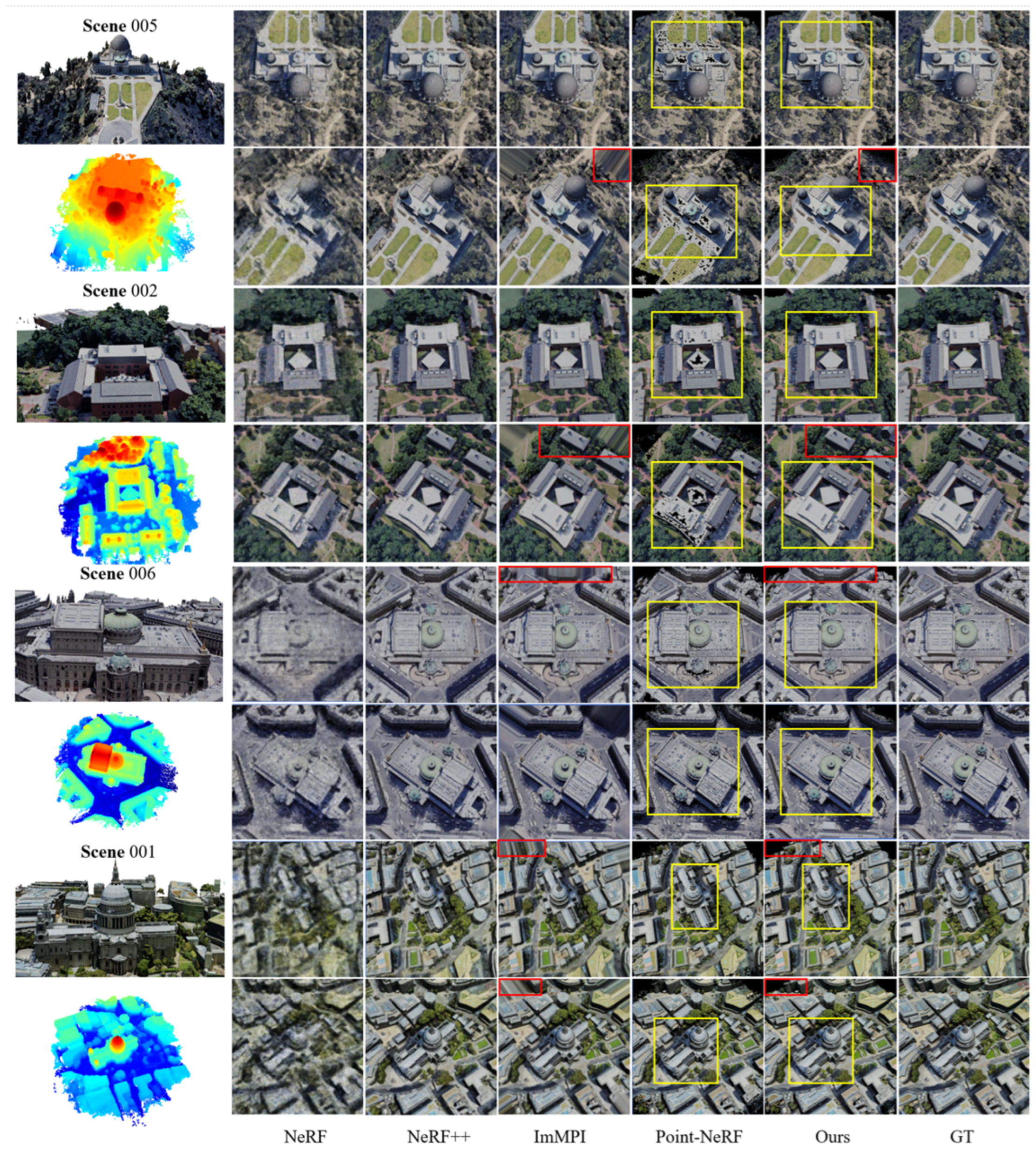
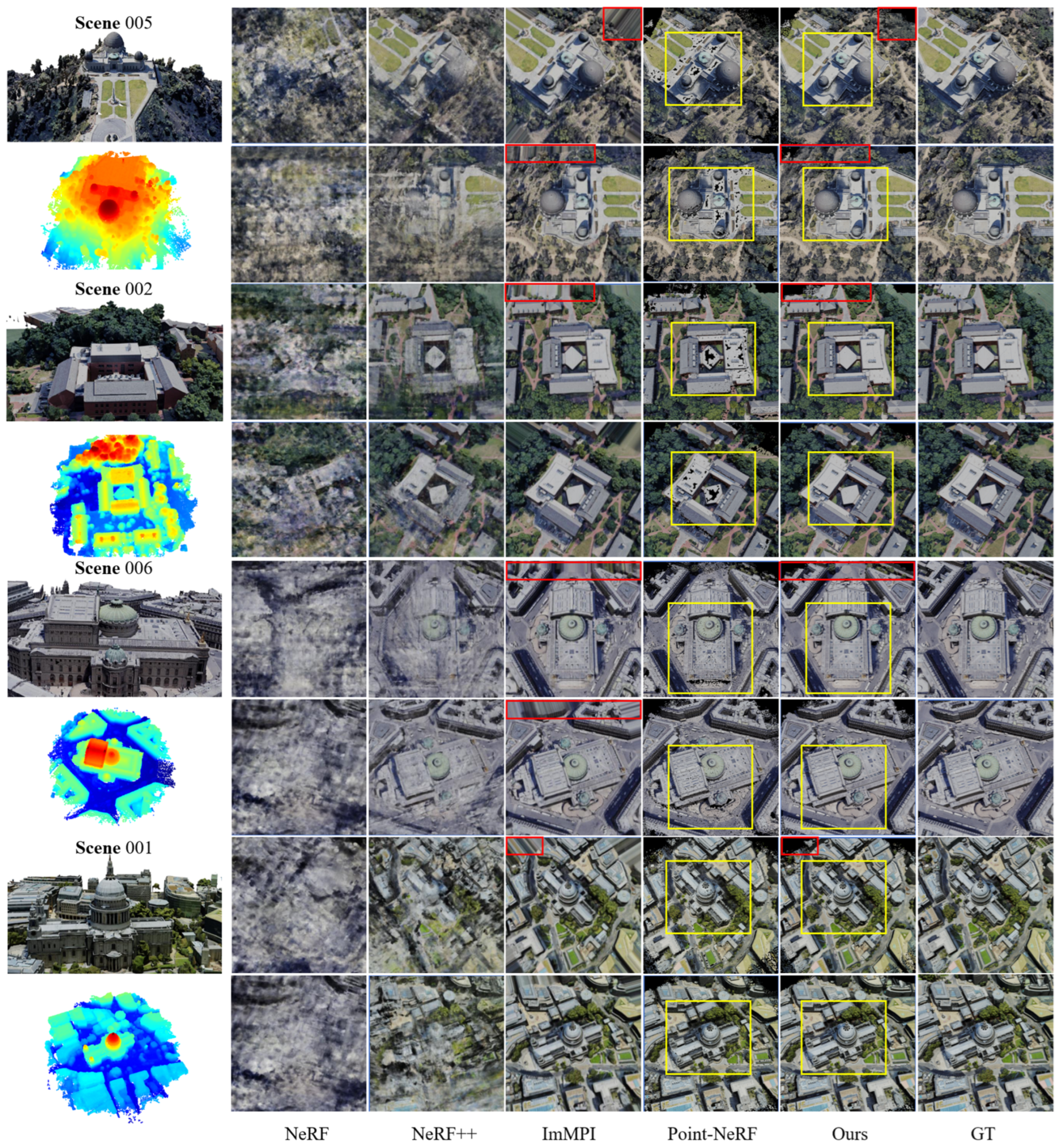
3.4. Performance Comparison

We compared our proposed method with four existing methods: NeRF [7], NeRF++ [27], ImMPI [15], and our baseline Point-NeRF [20]. The visual comparisons for the training and test sets are shown in Figure 6 and Figure 7, respectively. We also demonstrate the neural point cloud structure for the corresponding scenes. The red boxes represent comparisons between our method and ImMPI, showing that our method can reduce artifacts at the edges of the image. The yellow boxes represent comparisons between our method and the baseline, Point-NeRF. We found that NeRF [7] and NeRF++ [27] performed well on the training views but exhibited serious artifacts on the test views, indicating poor generalization. Point-NeRF [20] maintained relatively consistent performance across both the training and test sets due to stable, explicit 3D scene modeling. However, it suffered from holes in flat planes and shadows when faced with remote sensing imagery, meaning that Point-NeRF was outperformed by ImMPI. Our method effectively filled these holes and improved shadow processing, thereby achieving a more detailed perception.

In

Table 1. Quality assessment metrics of the training/test views for different methods.

Name of	PSNR			SSIM			LPIPS
Scene	ImMPI	Point-NeRF	Ours	ImMPI	Point-NeRF	Ours	ImMPI	Point-NeRF	Ours
Building #1	24.92/24.77	14.49/14.42	25.89/25.43	0.867/0.865	0.709/0.702	0.889/0.883	0.150/0.151	0.354/0.359	0.147/0.152
Building #2	23.31/22.73	19.12/18.57	24.97/24.88	0.783/0.776	0.866/0.862	0.867/0.864	0.217/0.218	0.233/0.237	0.211/0.216
College	26.17/25.71	17.57/17.52	24.92/23.84	0.820/0.817	0.813/0.806	0.825/0.818	0.201/0.203	0.272/0.274	0.198/0.205
Mountain #1	30.23/29.88	23.21/23.18	30.57/30.23	0.854/0.854	0.891/0.888	0.896/0.896	0.187/0.185	0.228/0.228	0.193/0.197
Mountain #2	29.56/29.37	22.82/22.82	29.47/29.33	0.844/0.843	0.913/0.911	0.916/0.915	0.172/0.173	0.189/0.192	0.169/0.173
Mountain #3	33.02/32.81	29.52/29.11	33.81/33.77	0.880/0.878	0.966/0.963	0.988/0.982	0.156/0.157	0.087/0.084	0.155/0.159
Observation	23.04/22.54	18.32/18.18	24.48/24.10	0.728/0.718	0.673/0.669	0.794/0.789	0.267/0.272	0.325/0.338	0.243/0.250
Church	21.60/21.04	18.87/18.82	22.62/22.57	0.729/0.720	0.838/0.834	0.849/0.843	0.254/0.258	0.262/0.265	0.236/0.245
Town #1	26.34/25.88	21.63/21.59	27.62/27.35	0.849/0.844	0.907/0.901	0.922/0.914	0.163/0.167	0.191/0.191	0.161/0.164
Town #2	25.89/25.31	20.11/20.05	26.81/26.58	0.855/0.850	0.896/0.892	0.915/0.914	0.156/0.158	0.179/0.176	0.147/0.151
Town #3	26.23/25.68	26.44/26.13	27.19/26.93	0.840/0.834	0.965/0.964	0.963/0.960	0.187/0.190	0.088/0.092	0.091/0.096
Stadium	26.69/26.50	21.38/21.12	26.31/26.12	0.878/0.876	0.873/0.869	0.888/0.887	0.123/0.125	0.168/0.173	0.145/0.164
Factory	28.15/28.08	19.22/19.22	27.65/27.53	0.908/0.907	0.891/0.889	0.910/0.902	0.109/0.109	0.191/0.193	0.129/0.131
Park	27.87/27.81	19.34/19.32	27.93/27.62	0.896/0.896	0.901/0.901	0.925/0.923	0.123/0.124	0.176/0.177	0.126/0.128
School	25.74/25.33	20.61/20.58	25.84/25.82	0.830/0.825	0.796/0.788	0.856/0.852	0.163/0.165	0.209/0.207	0.183/0.185
Downtown	24.99/24.24	20.58/20.56	25.12/25.08	0.825/0.816	0.898/0.898	0.903/0.901	0.201/0.205	0.212/0.211	0.199/0.204
mean	26.34/25.95	20.83/20.70	26.95/26.69	0.835/0.831	0.862/0.858	0.894/0.890	0.172/0.173	0.210/0.212	0.170/0.176

, we show the results of our quantitative comparison, mainly in relation to ImMPI and our baseline, Point-NeRF. First, due to the presence of holes, the performance of Point-NeRF was completely insufficient, resulting in PSNRs lower by 5.51 and 5.25 compared to ImMPI. However, it surpassed ImMPI by 0.027 in terms of the SSIM, indicating that the images rendered by explicit 3D scene representation have a more refined structure compared to the output of ImMPI. Our method significantly outperformed Point-NeRF across the 16 scenes. We achieved PSNRs that were 6.12/5.99 higher than those of Point-NeRF (training and test sets, respectively) and LPIPS values that were 0.040/0.036 lower. Thanks to the treatment of filling holes and shadows, our method maintained the advantage of Point-NeRF in terms of the SSIM, indicating that our approach can improve the quality of rendered images while preserving the integrity of spatial structural information.

4. Discussion

We now provide a detailed discussion of the innovative points of this study. First, we conduct ablation experiments on each sub-component to demonstrate the effectiveness of the method. Second, we compare the rendering efficiency consumption of the proposed method with that of other classical algorithms. Then, we separately analyze the structural consistency shadow model, the planar constraint, and inverse-projection hole-filling.

4.1. Ablation Study

We conducted ablation studies on the LEVIR_NEVS training set, as shown in

Table 2. Ablation study of sub-components.

	SC ${ }^1$	PC ${ }^2$	HF ${ }^3$	PSNR↑	SSIM↑	LPIPS↓
Init (Point-NeRF)	-			20.83	0.862	0.210
Configuration	✓			23.64	0.877	0.192
		✓		23.58	0.875	0.209
			✓	22.49	0.870	0.205
	✓	✓		24.89	0.884	0.197
	✓		✓	25.06	0.892	0.184
		✓	✓	25.42	0.903	0.188
	✓	✓	✓	26.95	0.984	0.170

¹ structural consistency shadow model; ² planar constraint; ³ inverse-projection hole-filling. Check mark indicates that the subpart is included in the current experiment, and the upward arrow indicates that the higher the value, the better, and vice versa.

. Initially, we found that all individual aspects of the proposed innovative points contributed to the overall improvement. When using the structural consistency shadow model (SC) alone, the model achieved gains of 2.81, 0.015, and −0.018 in terms of the PSNR, SSIM, and LPIPS, respectively. Meanwhile, the gains achieved using the planar constraint (PC) and inverse-projection hole-filling (HF) alone were 2.75, 0.13, and −0.001, and 1.66, 0.008, and 0.005, respectively. In the subsequent sections, we analyze these individual components in detail. Furthermore, we observed that combining these methods did not cause interference. The combination of HF and PC contributed the most to model performance, with gains of 4.59, 0.41, and 0.04. This indicates that our method can effectively address the issues present in a 3D scene structure.

4.2. Efficiency in Optimization and Rendering

We compared the optimization time and runtime speed of the proposed method against ImMPI, NeRF, NeRF++, and Point-NeRF. As shown in

Table 3. Quantitative comparison of optimization durations and rendering speeds between different methods.

Method	Image Size	Pre-Training	Optimization	Rendering
NeRF [7]	512 × 512	-	>90 min	>20 s
NeRF++ [27]	512 × 512	-	>60 min	>20 s
ImMPI [15]	512 × 512	21 h	<30 min	<1 s
Point-NeRF [20]	512 × 512	-	<60 min	12–14 s
Ours	512 × 512	-	<60 min	9–12 s

, our method outperformed NeRF and NeRF++ in terms of rendering speed and optimization duration when considering images of the same size (512 × 512). Although our method was not as fast as ImMPI in terms of rendering speed, it did not require a pre-training time of up to 21 h. For cross-scene problems, we only needed approximately 5 min to generate an initial point cloud based on COLMAP [23]. Therefore, our method demonstrates better efficiency in addressing cross-scene problems.

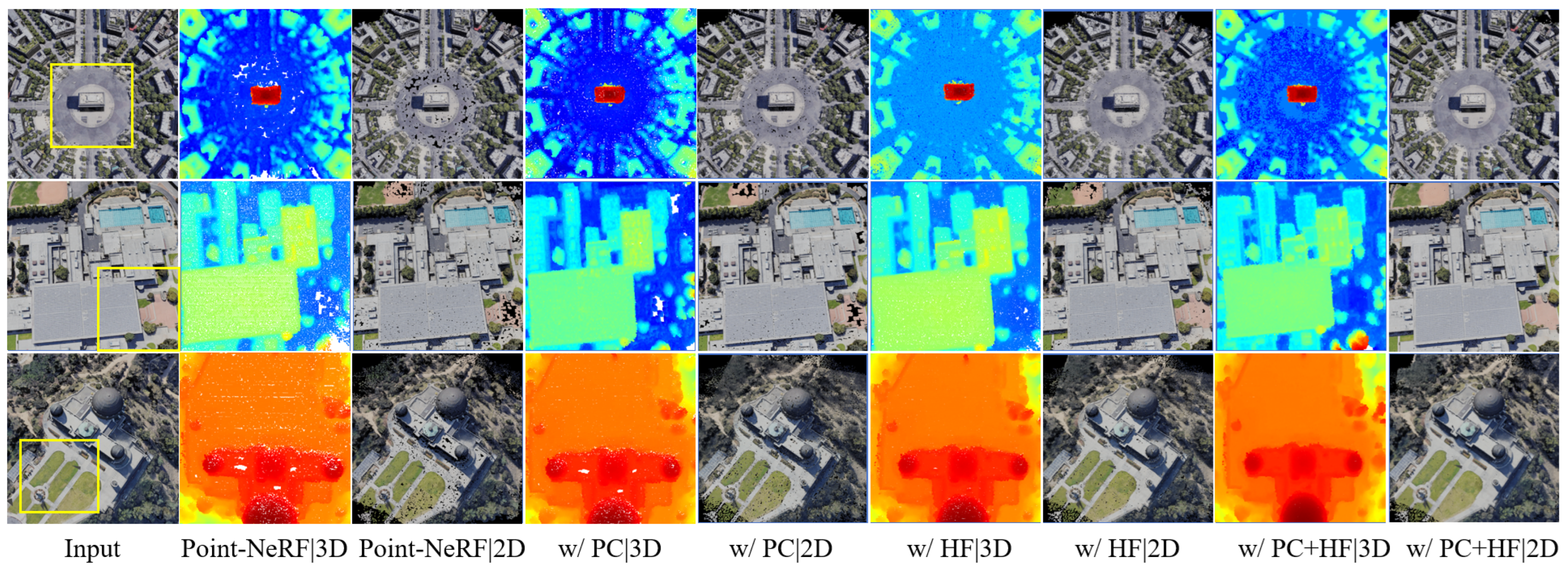
4.3. Effectiveness of Structural Consistency Shadow Model

During the rendering process, we attached two modules to output the albedo, ${\mathbf{c}}_{\mathbf{a}}$, and solar intensity, $s\left(\mathbf{r}\right)$, of the rendering points, as shown in Figure 8. The brighter the color, the higher the albedo and solar intensity values. We use two different color maps (gray and viridis) for distinction. We do not show the ambient light, as it is uniform and position-independent. As rendering is based on a 3D point cloud structure, some holes appear around the edges. However, hole-filling is not the strength of the shadow model. In the second and third rows, we can see that the structural consistency of light and shadow effectively identifies the shadow and processes the holes within it. For instance, in the input image in the first column of Figure 8, there are many holes inside the shadow of the central building. However, after correction using radiometric information, the point cloud has been supplemented. Similarly, in the input image in the second column, there are many holes within the shadow under the eaves, which, after correction, have been reduced. Our method not only achieves good perception in lower elevation areas but also performs well in downtown scenarios (as shown in the sixth column of Figure 8), helping to remove the missing parts caused by the shadowing of tall buildings.

4.4. Effectiveness of Planar Constraint and Hole-Filling

Plane constraint (PC) and hole-filling (HF), which use inverse-projection techniques, both aim to reduce failures in flat areas. For intuitive display, we selected three planar areas from the data set for demonstration: the roundabout in Scene 0 (Area #1), the square in Scene 5 (Area #2), and the factory roof in Scene 14 (Area #3). First, we show the results of both methods in Figure 9. From left to right are the images of the sampled areas, the results predicted using the original Point-NeRF model equipped with the PC/HF method, and finally, the effects of the proposed method. It is evident that the large areas of holes were significantly reduced with the addition of the PC method, and the incorporation of the HF method suppressed the presence of discrete holes. The combined use of these two methods led to the best enhancement in the model’s performance.

Figure 8. Albedo and solar intensity information calculated by the model. From top to bottom are the input images, albedo, and solar intensity. The ambient light is not shown because it is uniform and position-independent.

Figure 8. Albedo and solar intensity information calculated by the model. From top to bottom are the input images, albedo, and solar intensity. The ambient light is not shown because it is uniform and position-independent.

Figure 9. Qualitative effects of plane constraint (PC) and hole-filling (HF). We selected three planar areas: the roundabout in Scene 0 (Area #1), the square in Scene 5 (Area #2), and the factory roof in Scene 14 (Area #3). Each area is marked with the yellow rectangles. From left to right are the images of the sampled areas, the rendered (2D) and neural point (3D) results predicted using the original Point-NeRF model equipped with the PC/HF method, and finally, the effects of the proposed method.

Figure 9. Qualitative effects of plane constraint (PC) and hole-filling (HF). We selected three planar areas: the roundabout in Scene 0 (Area #1), the square in Scene 5 (Area #2), and the factory roof in Scene 14 (Area #3). Each area is marked with the yellow rectangles. From left to right are the images of the sampled areas, the rendered (2D) and neural point (3D) results predicted using the original Point-NeRF model equipped with the PC/HF method, and finally, the effects of the proposed method.

Subsequently, we analyzed the properties of the point clouds within these three areas. As shown in

Table 4. Quantitative comparison of local planar area attribution.

Test		Area #1			Area #2			Area #3
Method	Iteration	num_p	z_mean	z_var	num_p	z_mean	z_var	num_p	z_mean	z_var
Point-NeRF [20]	10 k	101,795	−22.48	15.69	153,496	−40.63	18.60	203,548	−55.83	16.58
	50 k	194,486	−21.75	12.81	203,694	−35.64	15.66	434,848	−53.61	13.52
	150 k	256,478	−20.78	8.64	289,492	−36.77	12.93	643,518	−51.84	10.96
w/PC	10 k	122,767	−20.28	13.85	183,647	−42.53	16.30	233,648	−53.64	13.64
	50 k	245,862	−19.36	10.11	262,148	−38.68	14.28	468,319	−51.62	13.25
	150 k	294,518	−19.27	8.36	331,496	−35.96	11.89	723,971	−49.36	11.30
w/HF	10 k	153,976	−23.44	14.23	203,546	−40.01	17.31	264,726	−58.16	16.17
	50 k	279,549	−21.30	11.38	364,795	−34.28	15.92	412,818	−52.11	13.76
	150 k	332,156	−19.12	8.15	369,842	−33.16	12.87	736,487	−53.19	13.89
w/PC + HF	10 k	235,716	−21.55	12.65	294,298	−35.68	15.28	301,428	−54.60	14.17
	50 k	303,674	−20.10	9.20	364,792	−33.14	13.64	453,972	−49.73	12.98
	150 k	401,498	−19.03	7.29	423,699	−32.27	12.39	782,364	−48.32	9.98
COLMAP	-	31,498	−18.63	6.97	39,483	−29.14	10.29	42,369	−42.98	7.70

, we defined the 3D scene boundaries based on inverse projection using Equation (16) and then extracted all the points within the generated neural point cloud. We counted the number of points and calculated the mean and variance of the z coordinate. These properties are presented at different training timestamps. In order to further compare the performance of Point-NeRF with the attached PC and HF methods, we also analyzed the data for each situation, along with the results generated by the traditional COLMAP [23] method. While the point cloud produced by COLMAP was relatively sparse, it could also reflect the overall properties of the area. The basic Point-NeRF progressively densified the original sparse point cloud, acquiring a 3D structure close to the real scene. However, as demonstrated in Figure 9, the rendered images that relied on these neural points suffered from many holes. After incorporating the PC and HF methods, the number of produced points at the three training timestamps was much higher. Taking Area #1 as an example, the growth rate of the point cloud quantity was 14% for the PC method, 29% after adding the HF method, and 56% with the combined use of both methods at 150,000 iterations. Similar trends were also observed in the other two scenes, indicating that our methods are capable of detecting the hole areas and, thus, can perform filling. However, increasing the number of points was not the ultimate goal. From the comparison of the statistical measures between the Point-NeRF and COLMAP point clouds, we observed that the COLMAP point clouds had a higher mean z coordinate, whereas those of Point-NeRF exhibited approximately a 5–15 m deviation, and the values from COLMAP were relatively stable. We also observed that our method adhered closely to the mean and variance of the point clouds produced by COLMAP after HF and PC processing. Taking Area #2 as an example, the z-mean value of the point cloud for this area generated by Point-NeRF was −36.77, with a variance of 12.93. After processing using our method, the mean was −32.27 and the variance was 10.29, closer to the results produced by COLMAP, thereby reflecting that the output of the neural point cloud aligned more with the actual structure. Of course, we do not rule out the possibility that the points may not be perfectly flat (for instance, there might be some inclination), but the reduction in variance indeed indicates that the elevation component of the points (in the world coordinate system) is gradually becoming consistent.

5. Conclusions

We have proposed an improved method to address the limitations of Point-NeRF in remote sensing image novel view synthesis tasks. This method tackles the problems of severe plane point loss and challenging hole processing in shadow areas by introducing plane constraint confidence handling, hole detection and filling, and a structural consistency shadow model to aid Point-NeRF in rendering. Specifically, the plane constraint confidence incorporates the original surface confidence to reduce the probability of plane points being pruned. Hole detection and filling incorporate 2D detection and inverse projection during training to identify holes and provide candidate spatial points for subsequent optimization. The shadow model, based on structural consistency, decomposes the radiance of object surfaces into albedo and irradiance, allowing the model to avoid directly predicting radiance and possess more reasonable physical properties. The experimental results demonstrate that our method can outperform the classical ImMPI algorithm in 2D novel viewpoint synthesis tasks.

In the 2D novel viewpoint synthesis task, our method achieved PSNRs of 26.95/26.93, SSIMs of 0.894/0.890, and LPIPSs of 0.170/0.176 for the training and test sets, respectively, on the LEVIR_NVS benchmark data set. Our method also generated a more accurate neural point cloud representation of the ground’s structural distribution. In subsequent research, we plan to incorporate more types of data, such as airborne LiDAR point clouds, for joint processing. We also aim to develop more efficient algorithms.

References

1. Wang, W.; Yang, N.; Zhang, Y.; Wang, F.; Cao, T.; Eklund, P. A review of road extraction from remote sensing images. J. Traffic Transp. Eng. (Engl. Ed.) 2016, 3, 271–282. [Google Scholar] [CrossRef]
2. Chen, Z.; Deng, L.; Luo, Y.; Li, D.; Junior, J.M.; Gonçalves, W.N.; Nurunnabi, A.A.M.; Li, J.; Wang, C.; Li, D. Road extraction in remote sensing data: A survey. Int. J. Appl. Earth Obs. Geoinf. 2022, 112, 102833. [Google Scholar] [CrossRef]
3. Xu, Y.; Xie, Z.; Feng, Y.; Chen, Z. Road extraction from high-resolution remote sensing imagery using deep learning. Remote Sens. 2018, 10, 1461. [Google Scholar] [CrossRef]
4. Zhang, L.; Lan, M.; Zhang, J.; Tao, D. Stagewise unsupervised domain adaptation with adversarial self-training for road segmentation of remote-sensing images. IEEE Trans. Geosci. Remote Sens. 2021, 60, 1–13. [Google Scholar] [CrossRef]
5. Wellmann, T.; Lausch, A.; Andersson, E.; Knapp, S.; Cortinovis, C.; Jache, J.; Scheuer, S.; Kremer, P.; Mascarenhas, A.; Kraemer, R.; et al. Remote sensing in urban planning: Contributions towards ecologically sound policies? Landsc. Urban Plan. 2020, 204, 103921. [Google Scholar] [CrossRef]
6. Li, K.; Wan, G.; Cheng, G.; Meng, L.; Han, J. Object detection in optical remote sensing images: A survey and a new benchmark. ISPRS J. Photogramm. Remote Sens. 2020, 159, 296–307. [Google Scholar] [CrossRef]
7. Mildenhall, B.; Srinivasan, P.P.; Tancik, M.; Barron, J.T.; Ramamoorthi, R.; Ng, R. Nerf: Representing scenes as neural radiance fields for view synthesis. Commun. ACM 2021, 65, 99–106. [Google Scholar] [CrossRef]
8. Achlioptas, P.; Diamanti, O.; Mitliagkas, I.; Guibas, L. Learning representations and generative models for 3d point clouds. In Proceedings of the International Conference on Machine Learning, ICML 2018, Stockholm, Sweden, 10–15 July 2018; pp. 40–49. [Google Scholar]
9. Qi, C.R.; Su, H.; Nießner, M.; Dai, A.; Yan, M.; Guibas, L.J. Volumetric and multi-view cnns for object classification on 3d data. In Proceedings of the IEEE Conference on Computer Vision and Pattern Recognition, Las Vegas, NV, USA, 27–30 June 2016; pp. 5648–5656. [Google Scholar]
10. Liu, L.; Gu, J.; Zaw Lin, K.; Chua, T.S.; Theobalt, C. Neural sparse voxel fields. Adv. Neural Inf. Process. Syst. 2020, 33, 15651–15663. [Google Scholar]
11. Kazhdan, M.; Bolitho, M.; Hoppe, H. Poisson surface reconstruction. In Proceedings of the Fourth Eurographics Symposium on Geometry Processing, Cagliari, Italy, 26–28 June 2006; Volume 7, p. 4. [Google Scholar]
12. Chen, Z.; Zhang, H. Learning implicit fields for generative shape modeling. In Proceedings of the IEEE/CVF Conference on Computer Vision and Pattern Recognition, Long Beach, CA, USA, 15–20 June 2019; pp. 5939–5948. [Google Scholar]
13. Levoy, M.; Hanrahan, P. Light field rendering. In Seminal Graphics Papers: Pushing the Boundaries, Volume 2; Association for Computing Machinery: New York, NY, USA, 2023; pp. 441–452. [Google Scholar]
14. Neff, T.; Stadlbauer, P.; Parger, M.; Kurz, A.; Mueller, J.H.; Chaitanya, C.R.A.; Kaplanyan, A.; Steinberger, M. DONeRF: Towards Real-Time Rendering of Compact Neural Radiance Fields using Depth Oracle Networks. Comput. Graph. Forum 2021, 40, 45–59. [Google Scholar] [CrossRef]
15. Wu, Y.; Zou, Z.; Shi, Z. Remote sensing novel view synthesis with implicit multiplane representations. IEEE Trans. Geosci. Remote Sens. 2022, 60, 1–13. [Google Scholar] [CrossRef]
16. Lv, J.; Guo, J.; Zhang, Y.; Zhao, X.; Lei, B. Neural Radiance Fields for High-Resolution Remote Sensing Novel View Synthesis. Remote Sens. 2023, 15, 3920. [Google Scholar] [CrossRef]
17. Li, X.; Li, C.; Tong, Z.; Lim, A.; Yuan, J.; Wu, Y.; Tang, J.; Huang, R. Campus3d: A photogrammetry point cloud benchmark for hierarchical understanding of outdoor scene. In Proceedings of the 28th ACM International Conference on Multimedia, Seattle, WA, USA, 12–16 October 2020; pp. 238–246. [Google Scholar]
18. Iman Zolanvari, S.; Ruano, S.; Rana, A.; Cummins, A.; da Silva, R.E.; Rahbar, M.; Smolic, A. DublinCity: Annotated LiDAR point cloud and its applications. arXiv 2019, arXiv:1909.03613. [Google Scholar]
19. Yang, G.; Xue, F.; Zhang, Q.; Xie, K.; Fu, C.W.; Huang, H. UrbanBIS: A Large-Scale Benchmark for Fine-Grained Urban Building Instance Segmentation. In ACM SIGGRAPH 2023 Conference Proceedings; Association for Computing Machinery: New York, NY, USA, 2023; pp. 1–11. [Google Scholar]
20. Xu, Q.; Xu, Z.; Philip, J.; Bi, S.; Shu, Z.; Sunkavalli, K.; Neumann, U. Point-nerf: Point-based neural radiance fields. In Proceedings of the IEEE/CVF Conference on Computer Vision and Pattern Recognition, New Orleans, LA, USA, 18–24 June 2022; pp. 5438–5448. [Google Scholar]
21. Yao, Y.; Luo, Z.; Li, S.; Fang, T.; Quan, L. Mvsnet: Depth inference for unstructured multi-view stereo. In Proceedings of the European Conference on Computer Vision (ECCV), Munich, Germany, 8–14 September 2018; pp. 767–783. [Google Scholar]
22. Simonyan, K.; Zisserman, A. Very deep convolutional networks for large-scale image recognition. arXiv 2014, arXiv:1409.1556. [Google Scholar]
23. Schonberger, J.L.; Frahm, J.M. Structure-from-motion revisited. In Proceedings of the IEEE Conference on Computer Vision and Pattern Recognition, Las Vegas, NV, USA, 27–30 June 2016; pp. 4104–4113. [Google Scholar]
24. Derksen, D.; Izzo, D. Shadow Neural Radiance Fields for Multi-View Satellite Photogrammetry. In Proceedings of the IEEE/CVF Conference on Computer Vision and Pattern Recognition (CVPR) Workshops, Nashville, TN, USA, 19–25 June 2021; pp. 1152–1161. [Google Scholar]
25. Marí, R.; Facciolo, G.; Ehret, T. Sat-NeRF: Learning Multi-View Satellite Photogrammetry with Transient Objects and Shadow Modeling Using RPC Cameras. In Proceedings of the IEEE/CVF Conference on Computer Vision and Pattern Recognition (CVPR) Workshops, New Orleans, LA, USA, 19–20 June 2022; pp. 1311–1321. [Google Scholar]
26. Marí, R.; Facciolo, G.; Ehret, T. Multi-Date Earth Observation NeRF: The Detail Is in the Shadows. In Proceedings of the IEEE/CVF Conference on Computer Vision and Pattern Recognition (CVPR) Workshops, Vancouver, BC, Canada, 18–22 June 2023; pp. 2035–2045. [Google Scholar]
27. Zhang, K.; Riegler, G.; Snavely, N.; Koltun, V. NeRF++: Analyzing and Improving Neural Radiance Fields. Clin. Orthop. Relat. Res. 2020. [Google Scholar] [CrossRef]
Figure 1. The main idea and effect of our method. A neural radiance field constructed from a point cloud often generates holes in the planes during the rendering of remote sensing images (a,c). We introduce a new neural point cloud completion method based on Point-NeRF, effectively addressing this issue (b,d). In order to eliminate the influence of different coordinate systems, the color band corresponds to the absolute elevation range of the neural point cloud; that is, if the z values of the lowest and highest points are z m i n and z m a x , respectively, the corresponding range of the color band is [0, z m a x z m i n ].
Remotesensing 16 01341 g001
Figure 2. Different effects when Point-NeRF reconstructs urban scenes and mountains. The first row contains the rendered images, and the second row contains the neural point clouds.
Remotesensing 16 01341 g002
Figure 3. The problem with Point-NeRF in reconstructing an area in shadow. Point-NeRF has difficulty dealing with shadows, especially those in shadow areas caused by sunlight.
Remotesensing 16 01341 g003
Figure 4. The main workflow of our method. We first employ COLMAP to generate a sparse point cloud and initialize the radiance field. Subsequently, we decompose the radiance into albedo and irradiance, optimizing the original ray-marching algorithm using a shadow model with structural consistency to obtain shadow-invariant features. Following this, we perform hole detection and filling on the rendered views, and we introduce a new planar confidence parameter to reduce the probability of pruning the planar points. Finally, the model is optimized by calculating the loss between the rendered radiance and the ground truth.
Remotesensing 16 01341 g004
Figure 5. Structural consistency shadow model based on point clouds.
Remotesensing 16 01341 g005
Figure 6. Qualitative comparison of training set images. These images were used during training and were rendered using the corresponding camera poses. The neural point cloud structure of each scene is demonstrated on the left. The red boxes represent comparisons between our method and ImMPI, and the yellow boxes represent comparisons between our method and the baseline, Point-NeRF.
Remotesensing 16 01341 g006
Figure 7. Qualitative comparison of test set images. The views in these images had not been seen by the models in the pre-training and optimization process. These images were used during training and were rendered using the corresponding camera poses. The neural point cloud structure of each scene is shown on the left. The red boxes represent comparisons between our method and ImMPI, and the yellow boxes represent comparisons between our method and the baseline, Point-NeRF.
Remotesensing 16 01341 g007