

Unraveling the Influence of Equatorial Waves on Post-Monsoon Sea Surface Salinity Anomalies in the Bay of Bengal

Abstract
:1. Introduction
2. Materials and Methods
2.1. Materials
2.2. Methods
3. Results
3.1. Regression and Correlation Analysis
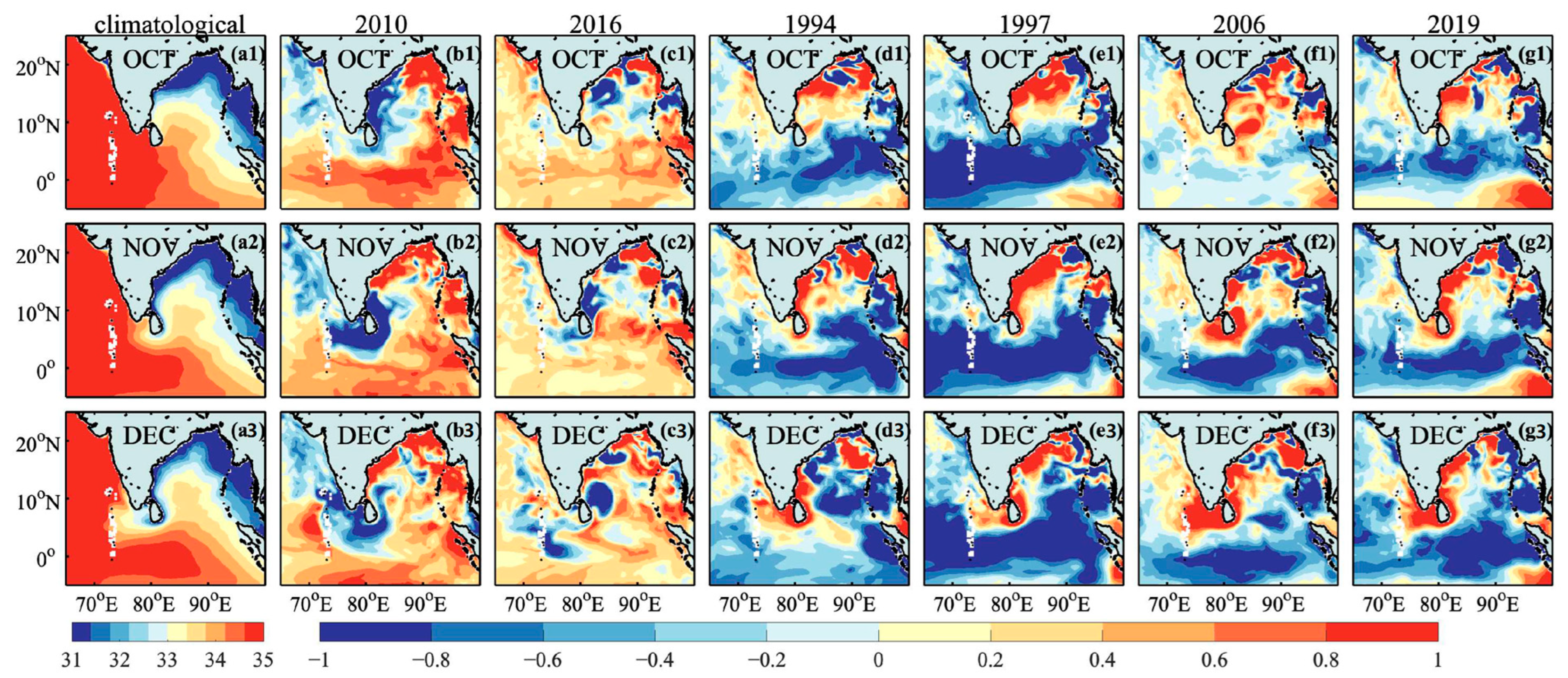
3.2. Characteristics of SSSAs in Anomalous Westerly Years and Easterly Years
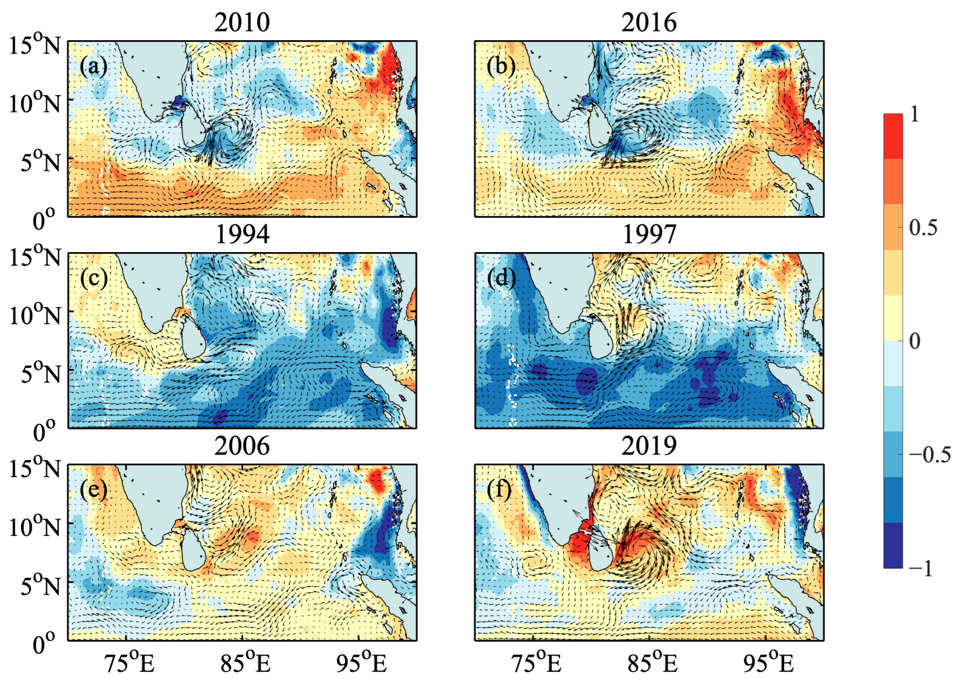
3.3. Large-Scale Currents
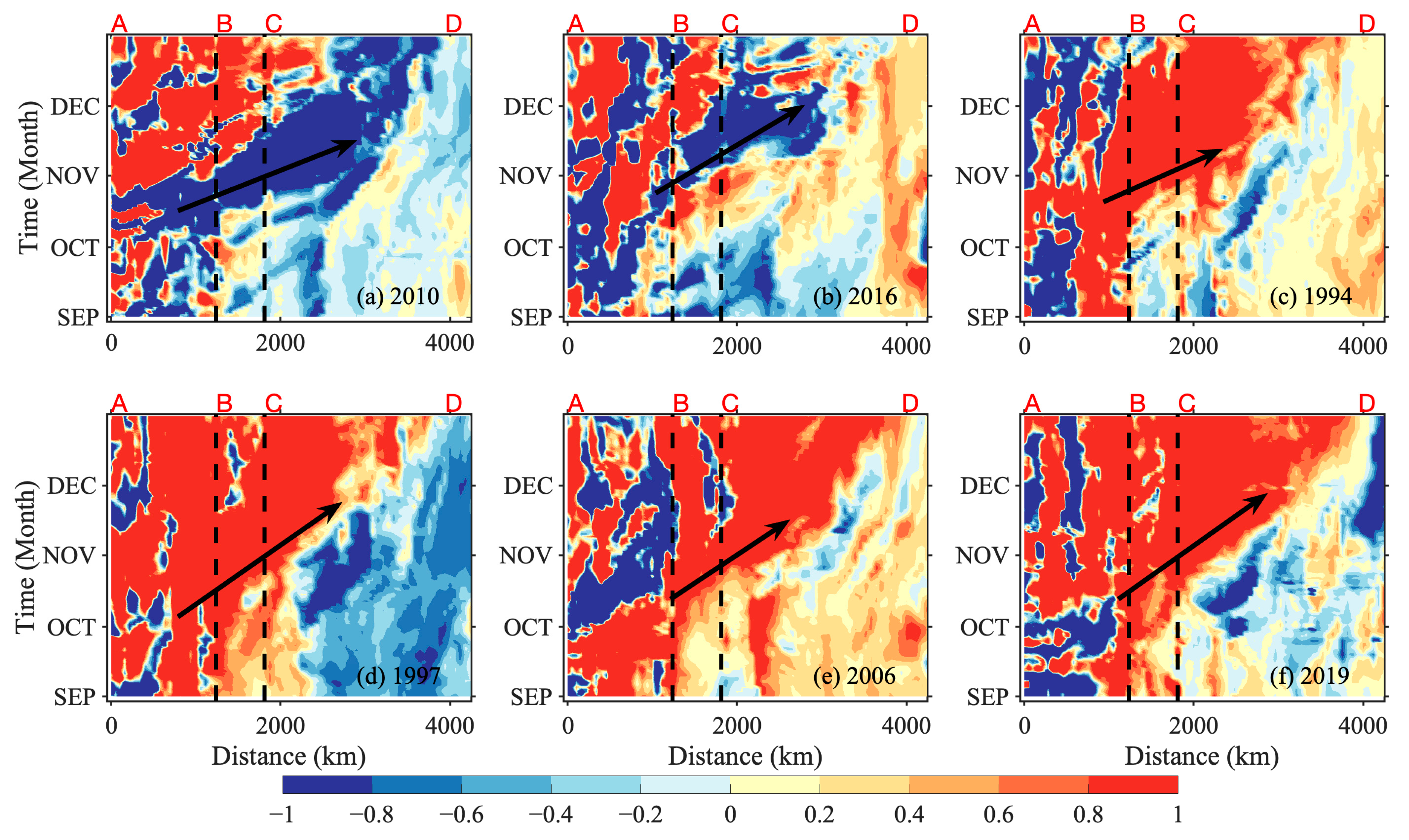
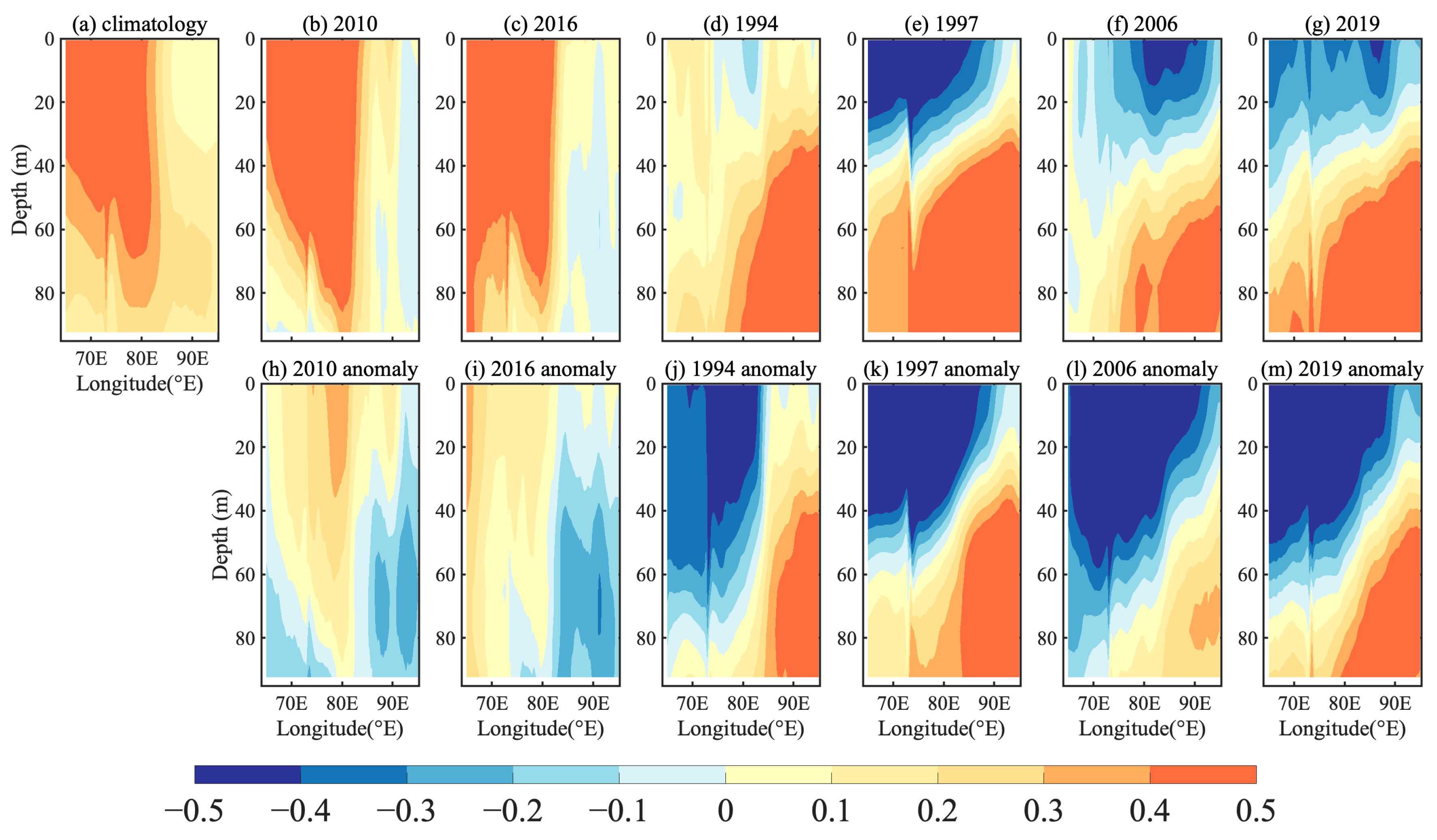
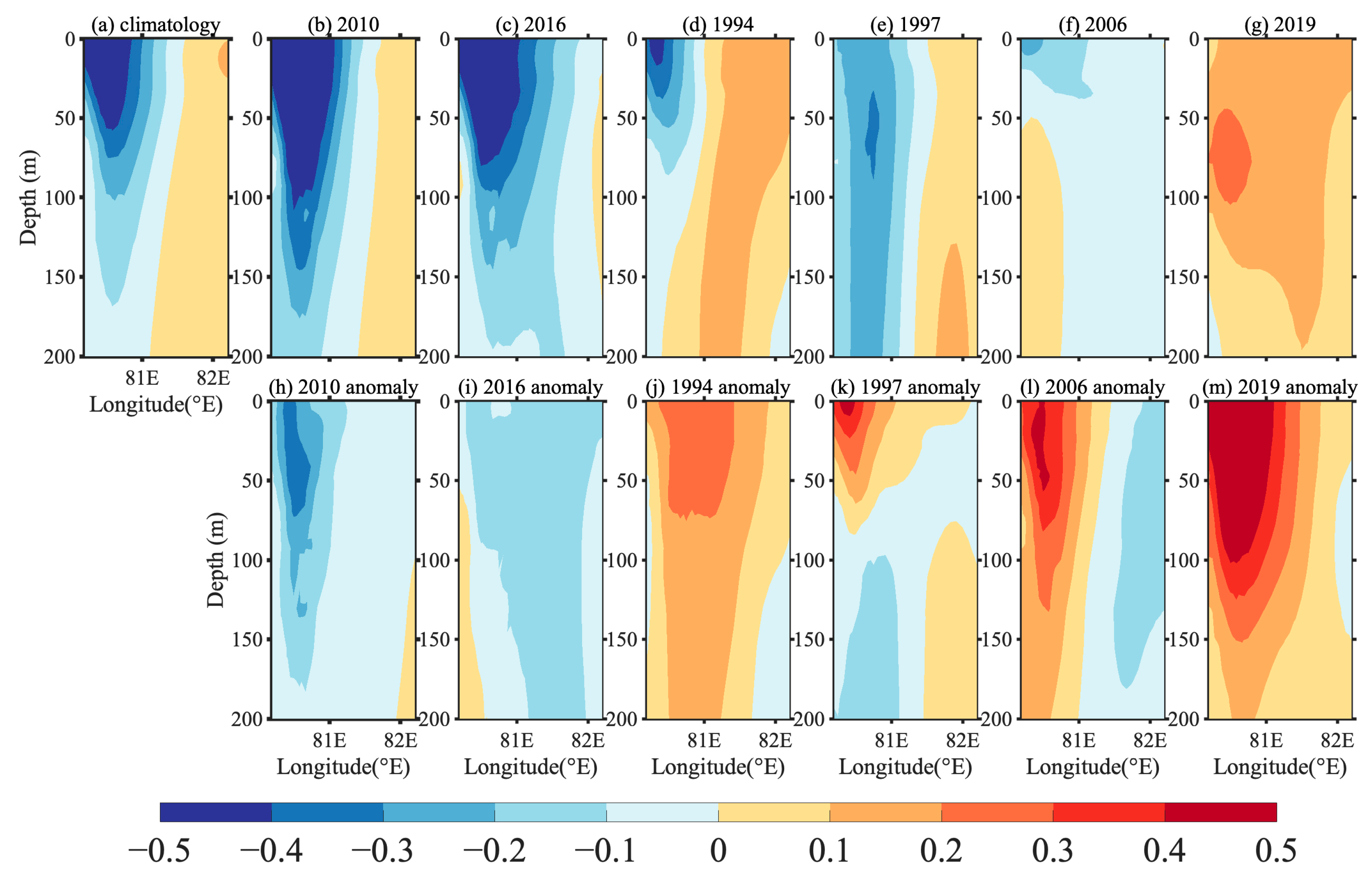
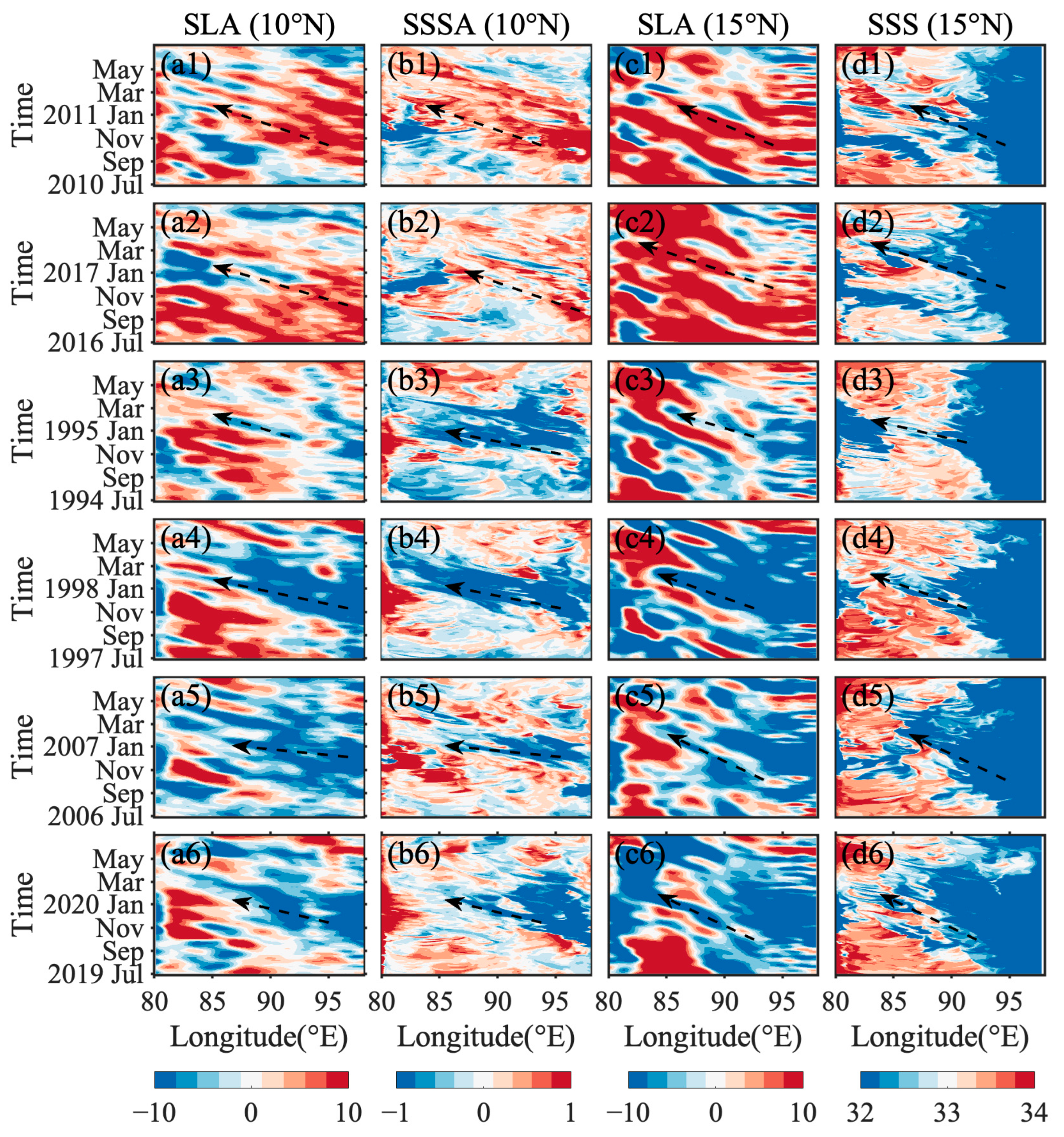
3.4. Kelvin Waves
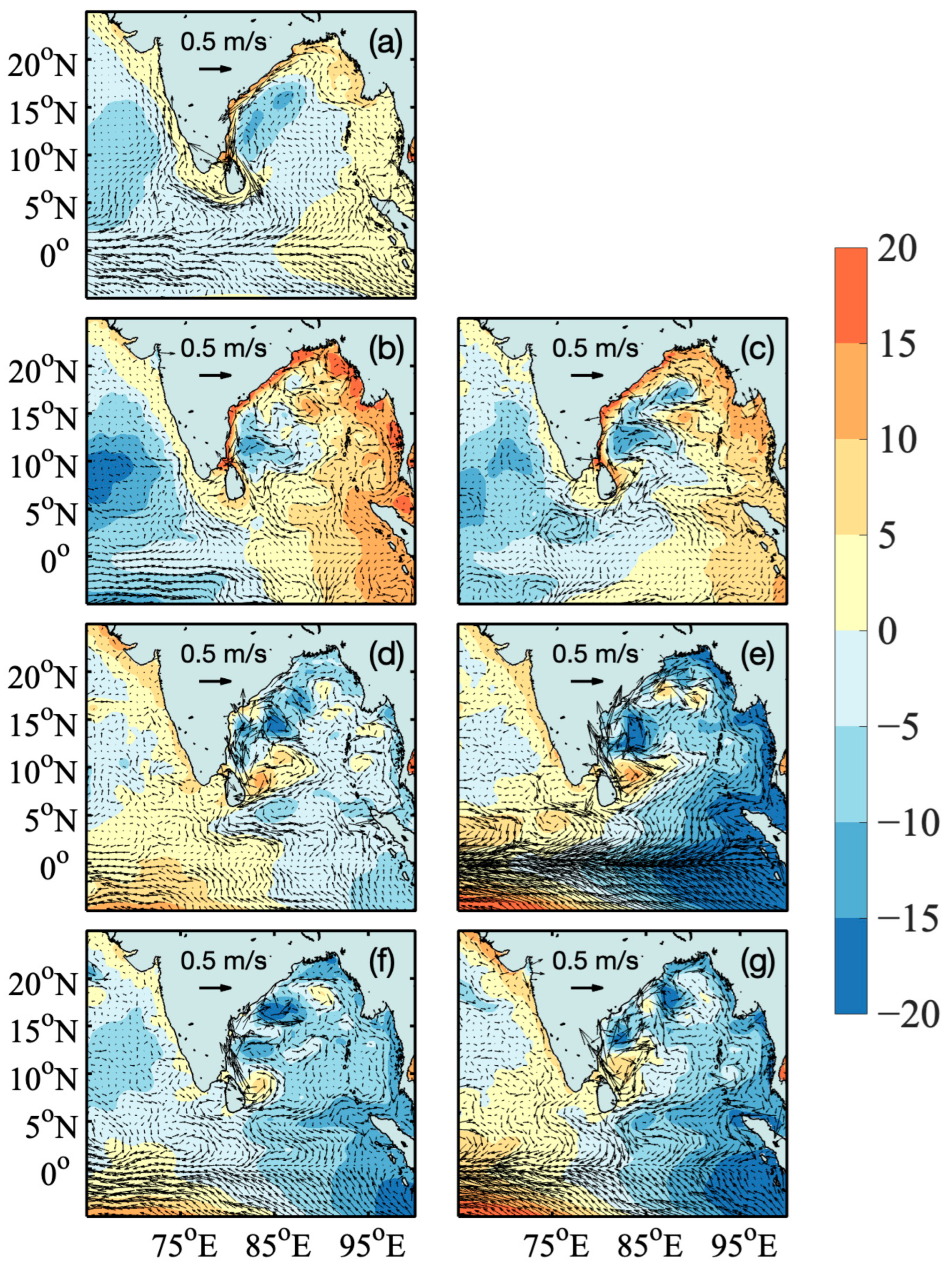
3.5. Rossby Waves
4. Discussion
Author Contributions
Funding
Data Availability Statement
Acknowledgments
Conflicts of Interest
References
- Li, Z.; Lian, T.; Ying, J.; Zhu, X.; Papa, F.; Xie, H.; Long, Y. The Cause of an Extremely Low Salinity Anomaly in the Bay of Bengal During 2012 Spring. J. Geophys. Res. Ocean. 2021, 126, e2021JC017361. [Google Scholar] [CrossRef]
- Sprintall, J.; Tomczak, M. Evidence of the barrier layer in the surface layer of the tropics. J. Geophys. Res. 1992, 97, 7305–7316. [Google Scholar] [CrossRef]
- Thadathil, P.; Muraleedharan, P.M.; Rao, R.R.; Somayajulu, Y.K.; Reddy, G.V.; Revichandran, C. Observed seasonal variability of barrier layer in the Bay of Bengal. J. Geophys. Res. 2007, 112. [Google Scholar] [CrossRef]
- Cronin, M.F.; McPhaden, M.J. Barrier layer formation during westerly wind bursts. J. Geophys. Res. Ocean. 2002, 107, SRF 21-1–SRF 21-12. [Google Scholar] [CrossRef]
- Rao, R.R. Seasonal variability of sea surface salinity and salt budget of the mixed layer of the north Indian Ocean. J. Geophys. Res. 2003, 108, 9-1–9-14. [Google Scholar] [CrossRef]
- Akhil, V.P.; Valiya Parambil, A.; Valiya Parambil, A.; Matthieu, L.; Jérôme, V.; Fabien, D.; Fabien, D.; Keerthi, M.G.; Akurathi Venkata Sai, C.; Fabrice, P.; et al. A modeling study of processes controlling the Bay of Bengal sea surface salinity interannual variability. J. Geophys. Res. 2016, 116, 3926–3947. [Google Scholar] [CrossRef]
- Akhil, V.P.; Vialard, J.; Lengaigne, M.; Keerthi, M.G.; Boutin, J.; Vergely, J.L.; Papa, F. Bay of Bengal Sea surface salinity variability using a decade of improved SMOS re-processing. Remote Sens. Environ. 2020, 248, 111964. [Google Scholar] [CrossRef]
- Chen, S.; Cha, J.; Qiu, F.; Jing, C.; Qiu, Y.; Xu, J. Sea Surface Salinity Anomaly in the Bay of Bengal during the 2010 Extremely Negative IOD Event. Remote Sens. 2022, 14, 6242. [Google Scholar] [CrossRef]
- Chaitanya, A.V.S.; Durand, F.; Mathew, S.; Gopalakrishna, V.V.; Papa, F.; Lengaigne, M.; Vialard, J.; Kranthikumar, C.; Venkatesan, R. Observed year-to-year sea surface salinity variability in the Bay of Bengal during the 2009–2014 period. Ocean Dyn. 2014, 65, 173–186. [Google Scholar] [CrossRef]
- Zhang, Z.; Wang, J.; Yuan, D. Mixed Layer Salinity Balance in the Eastern Tropical Indian Ocean. J. Geophys. Res. Ocean. 2022, 127, e2021JC018229. [Google Scholar] [CrossRef]
- Wyrtki, K. An equatorial jet in the Indian Ocean. Science 1973, 181, 262–264. [Google Scholar] [CrossRef]
- Jing, W.; Jing, W.; Jing, W. Observational bifurcation of Wyrtki Jets and its influence on the salinity balance in the eastern Indian Ocean. Atmos. Ocean. Sci. Lett. 2017, 10, 36–43. [Google Scholar] [CrossRef]
- Thompson, B.; Gnanaseelan, C.; Salvekar, P.S. Variability in the Indian Ocean circulation and salinity and its impact on SST anomalies during dipole events. J. Mar. Res. 2006, 64, 853–880. [Google Scholar] [CrossRef]
- Chatterjee, A.; Shankar, D.; McCreary, J.P.; Vinayachandran, P.N.; Mukherjee, A. Dynamics of Andaman Sea circulation and its role in connecting the equatorial Indian Ocean to the Bay of Bengal. J. Geophys. Res. Ocean. 2017, 122, 3200–3218. [Google Scholar] [CrossRef]
- Yu, L.; O’Brien, J.J.; Yang, J. On the remote forcing of the circulation in the Bay of Bengal. J. Geophys. Res. 1991, 96, 20449–20454. [Google Scholar] [CrossRef]
- Rao, R.R.; Girish Kumar, M.S.; Ravichandran, M.; Rao, A.R.; Gopalakrishna, V.V.; Thadathil, P. Interannual variability of Kelvin wave propagation in the wave guides of the equatorial Indian Ocean, the coastal Bay of Bengal and the southeastern Arabian Sea during 1993–2006. Deep Sea Res. Part I Oceanogr. Res. Pap. 2010, 57, 1–13. [Google Scholar] [CrossRef]
- Fournier, S.; Vialard, J.; Lengaigne, M.; Lee, T.; Gierach, M.M.; Chaitanya, A.V.S. Modulation of the Ganges-Brahmaputra River Plume by the Indian Ocean Dipole and Eddies Inferred From Satellite Observations. J. Geophys. Res. Ocean. 2017, 122, 9591–9604. [Google Scholar] [CrossRef]
- Sreenivas, P.; Gnanaseelan, C.; Prasad, K.V.S.R. Influence of El Niño and Indian Ocean Dipole on sea level variability in the Bay of Bengal. Glob. Planet. Chang. 2012, 80–81, 215–225. [Google Scholar] [CrossRef]
- Pant, V.; Girishkumar, M.S.; Bhaskar, T.V.S.U.; Ravichandran, M.; Fabrice, P.; Thangaprakash, V.P. Observed interannual variability of near-surface salinity in the Bay of Bengal. J. Geophys. Res. 2015, 120, 3315–3329. [Google Scholar] [CrossRef]
- Hersbach, H.; Bell, B.; Berrisford, P.; Biavati, G.; Horányi, A.; Muñoz Sabater, J.; Nicolas, J.; Peubey, C.; Radu, R.; Rozum, I.; et al. ERA5 Hourly Data on Single Levels from 1940 to Present; Copernicus Climate Change Service (C3S) Climate Data Store (CDS). 2023. Available online: https://cds.climate.copernicus.eu/cdsapp#!/dataset/10.24381/cds.adbb2d47?tab=overview (accessed on 7 April 2024).
- Xin, L.; Hu, S.; Wang, F.; Xie, W.; Hu, D.; Dong, C. Using a deep-learning approach to infer and forecast the Indonesian Throughflow transport from sea surface height. Front. Mar. Sci. 2023, 10, 1079286. [Google Scholar] [CrossRef]
- Akhil, V.P.; Lengaigne, M.; Durand, F.; Vialard, J.; Chaitanya, A.V.S.; Keerthi, M.G.; Gopalakrishna, V.V.; Boutin, J.; de Boyer Montégut, C. Assessment of seasonal and year-to-year surface salinity signals retrieved from SMOS and Aquarius missions in the Bay of Bengal. Int. J. Remote Sens. 2016, 37, 1089–1114. [Google Scholar] [CrossRef]
- Ratna, S.B.; Cherchi, A.; Osborn, T.J.; Joshi, M.; Uppara, U. The Extreme Positive Indian Ocean Dipole of 2019 and Associated Indian Summer Monsoon Rainfall Response. Geophys. Res. Lett. 2021, 48, e2020GL091497. [Google Scholar] [CrossRef]
- Ernst, P.A.; Subrahmanyam, B.; Trott, C.B. Lakshadweep High Propagation and Impacts on the Somali Current and Eddies During the Southwest Monsoon. J. Geophys. Res. Ocean. 2022, 127, e2021JC018089. [Google Scholar] [CrossRef]
- Yuhong, Z.; Yan, D.; Shaojun, Z.; Yali, Y.; Xuhua, C. Impact of Indian Ocean Dipole on the salinity budget in the equatorial Indian Ocean. J. Geophys. Res. Ocean. 2013, 118, 4911–4923. [Google Scholar] [CrossRef]
- Potemra, J.T.; Luther, M.E.; O’Brien, J.J. The seasonal circulation of the upper ocean in the Bay of Bengal. J. Geophys. Res. 1991, 96, 12667–12683. [Google Scholar] [CrossRef]
- Suresh, I.; Vialard, J.; Lengaigne, M.; Izumo, T.; Parvathi, V.; Muraleedharan, P.M. Sea Level Interannual Variability Along the West Coast of India. Geophys. Res. Lett. 2018, 45, 12440–12448. [Google Scholar] [CrossRef]
- Cheng, X.; McCreary, J.P.; Qiu, B.; Qi, Y.; Du, Y.; Chen, X. Dynamics of Eddy Generation in the Central Bay of Bengal. J. Geophys. Res. Ocean. 2018, 123, 6861–6875. [Google Scholar] [CrossRef]
- Chen, G.; Han, W.; Li, Y.; McPhaden, M.J.; Chen, J.; Wang, W.; Wang, D. Strong Intraseasonal Variability of Meridional Currents near 5°N in the Eastern Indian Ocean: Characteristics and Causes. J. Phys. Oceanogr. 2017, 47, 979–998. [Google Scholar] [CrossRef]
- Huang, H.; Wang, D.; Yang, L.; Huang, K. Enhanced Intraseasonal Variability of the Upper Layers in the Southern Bay of Bengal During the Summer 2016. J. Geophys. Res. Ocean. 2021, 126, e2021JC017459. [Google Scholar] [CrossRef]
- Li, Z.; Long, Y.; Huang, S.; Xie, H.; Zhou, Y.; Yang, B.; Bai, Y.; Zhu, X.H. A Large Winter Chlorophyll-a Bloom in the Southeastern Bay of Bengal Associated With the Extreme Indian Ocean Dipole Event in 2019. J. Geophys. Res. Ocean. 2023, 128, e2022JC018791. [Google Scholar] [CrossRef]
- Li, Y.; Han, W.; Ravichandran, M.; Wang, W.; Shinoda, T.; Lee, T. Bay of Bengal salinity stratification and Indian summer monsoon intraseasonal oscillation: 2. Impact on SST and convection. J. Geophys. Res. Ocean. 2017, 122, 4312–4328. [Google Scholar] [CrossRef]
- McPhaden, M.J.; Foltz, G.R. Intraseasonal variations in the surface layer heat balance of the central equatorial Indian Ocean: The importance of zonal advection and vertical mixing. Geophys. Res. Lett. 2013, 40, 2737–2741. [Google Scholar] [CrossRef]
- Han, W.; Li, Y.; Wang, W.; Ravichandran, M. Intraseasonal Variability of SST and Precipitation in the Arabian Sea during the Indian Summer Monsoon: Impact of Ocean Mixed Layer Depth. J. Clim. 2016, 29, 7889–7910. [Google Scholar] [CrossRef]
- Ivanova, D.P.; McClean, J.L.; Sprintall, J.; Chen, R. The Oceanic Barrier Layer in the Eastern Indian Ocean as a Predictor for Rainfall Over Indonesia and Australia. Geophys. Res. Lett. 2021, 48, e2021GL094519. [Google Scholar] [CrossRef]
- Rao, R.; Sivakumar, R. On the possible mechanisms of the evolution of a mini-warm pool during the pre-summer monsoon season and the genesis of onset vortex in the South-Eastern Arabian Sea. Q. J. R. Meteorol. Soc. 1999, 125, 787–809. [Google Scholar]


| Parameter | Source | Resolution | Time Period |
|---|---|---|---|
| Zonal wind at 10 m | https://cds.climate.copernicus.eu accessed on 10 April 2023 | Hourly, 0.25° × 0.25° | 1991–2021 |
| SMOS SSS | https://earth.esa.int/ accessed on 15 April 2022 | 2010–2020 | |
| CMEMS current, salinity, and potential temperature | http://marine.copernicus.eu accessed on 23 March 2023 | Daily, 1/12° × 1/12°, 50 vertical levels | 1993–2020 |
| AVISO SLA, geostrophic zonal and meridional currents | https://www.aviso.altimetry.fr/ accessed on 20 March 2023 | Daily, 0.25° × 0.25° | 1993–2020 |
Disclaimer/Publisher’s Note: The statements, opinions and data contained in all publications are solely those of the individual author(s) and contributor(s) and not of MDPI and/or the editor(s). MDPI and/or the editor(s) disclaim responsibility for any injury to people or property resulting from any ideas, methods, instructions or products referred to in the content. |
© 2024 by the authors. Licensee MDPI, Basel, Switzerland. This article is an open access article distributed under the terms and conditions of the Creative Commons Attribution (CC BY) license (https://creativecommons.org/licenses/by/4.0/).
Share and Cite
Chen, S.; Qiu, F.; Jing, C.; Qiu, Y.; Zhang, J. Unraveling the Influence of Equatorial Waves on Post-Monsoon Sea Surface Salinity Anomalies in the Bay of Bengal. Remote Sens. 2024, 16, 1348. https://doi.org/10.3390/rs16081348
Chen S, Qiu F, Jing C, Qiu Y, Zhang J. Unraveling the Influence of Equatorial Waves on Post-Monsoon Sea Surface Salinity Anomalies in the Bay of Bengal. Remote Sensing. 2024; 16(8):1348. https://doi.org/10.3390/rs16081348
Chicago/Turabian StyleChen, Shuling, Fuwen Qiu, Chunsheng Jing, Yun Qiu, and Junpeng Zhang. 2024. "Unraveling the Influence of Equatorial Waves on Post-Monsoon Sea Surface Salinity Anomalies in the Bay of Bengal" Remote Sensing 16, no. 8: 1348. https://doi.org/10.3390/rs16081348