

Channel Estimation for Underwater Acoustic Communications in Impulsive Noise Environments: A Sparse, Robust, and Efficient Alternating Direction Method of Multipliers-Based Approach


Abstract
1. Introduction
- We introduce a robust algorithm by reformulating the channel estimation problem as an optimization problem, which offers enhanced resilience to outliers. This new optimization problem is adeptly tackled using the ADMM framework with the Accelerated Proximal Gradient (APG) method [34]. Furthermore, we incorporate a non-monotone line search strategy to increase the convergence speed as well as improve the robustness, particularly for ill-conditioned problems. The proposed method is low in complexity and has robust performance in challenging noise conditions.
- We evaluate the performance of the proposed algorithm in various scenarios including estimating channel impulse response (CIR) and Delay-Doppler (DD) spread functions for single-carrier systems through simulations as well as at-sea experimental validations for channel estimation in OFDM systems. The results demonstrate the fast convergence speed and high accuracy of the proposed method in both AWGN and impulsive noise environments, making it well-suited for robust channel estimations for diverse UWA channel models and communication schemes in practical applications.
2. Preliminaries
2.1. Channel Estimation in UAC Systems
2.2. Compressed Sensing Approach
3. Details of the Proposed Algorithm
3.1. General Framework
3.2. Update of Primal Variable:
| Algorithm 1 Update of Primary Variable x: Monotone Strategy [28] |
| Iteration 0: Set , , and . |
| … |
| Iteration k: Get , , and from previous iteration. |
| 1: Compute the gradient using (22). |
| 2: Backtracking Line Search: find the minimum number of iterations such that with |
| and |
| 3: Set . |
| Algorithm 2 Update of Primary Variable x: Non-monotone Strategy | |
| Iteration 0: Set , , , and . | |
| … | |
| Iteration k: Get , , , and from previous iteration. | |
| 1: | Compute the extrapolation point by (25) and the gradient by (22), respectively. |
| 2: | Backtracking Line Search: find the minimum number of iterations such that with and |
| 3: | if then |
| 4: | set |
| 5: | else |
| 6: | Compute the gradient by (22). |
| 7: | Backtracking Line Search: find the minimum number of iterations such that with and |
| 8: | Compute and
|
| 9: | end if |
| 10: | Update the extrapolation parameter by (26), and and by (29). |
3.3. Update of Auxiliary Variable:
| Algorithm 3 Update of Auxiliary Variable z |
| Iteration 0: Set , . |
| … |
| Iteration k: Get , , , , and from previous iteration. |
| 1: Compute the extrapolation point by (33) and the gradient by (32). |
| 2: Evaluate the proximal operator: |
| 3: Compute by (17) and |
| 4: Update the extrapolation parameter by (26). |
3.4. Residues, Stopping Criteria, and Penalty Parameter Tuning
| Algorithm 4 Proposed Algorithm |
|
3.5. Computational Complexity
4. Numerical Simulations
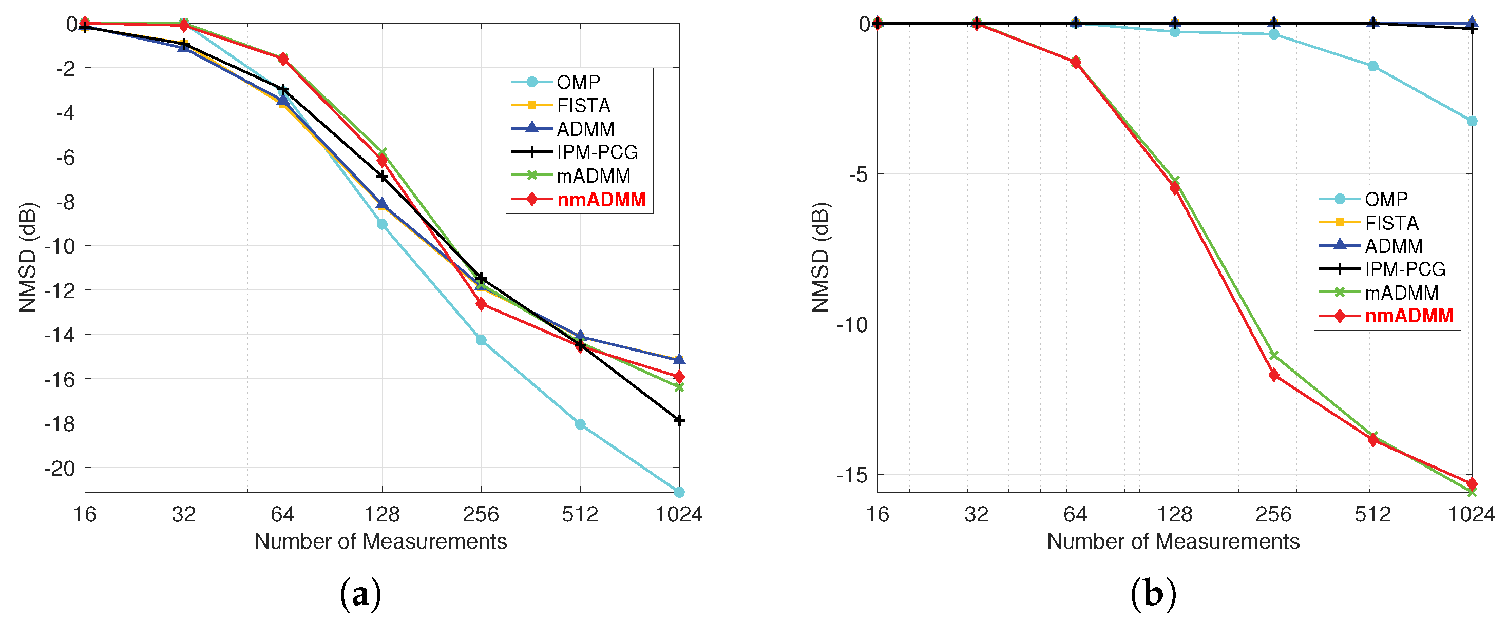
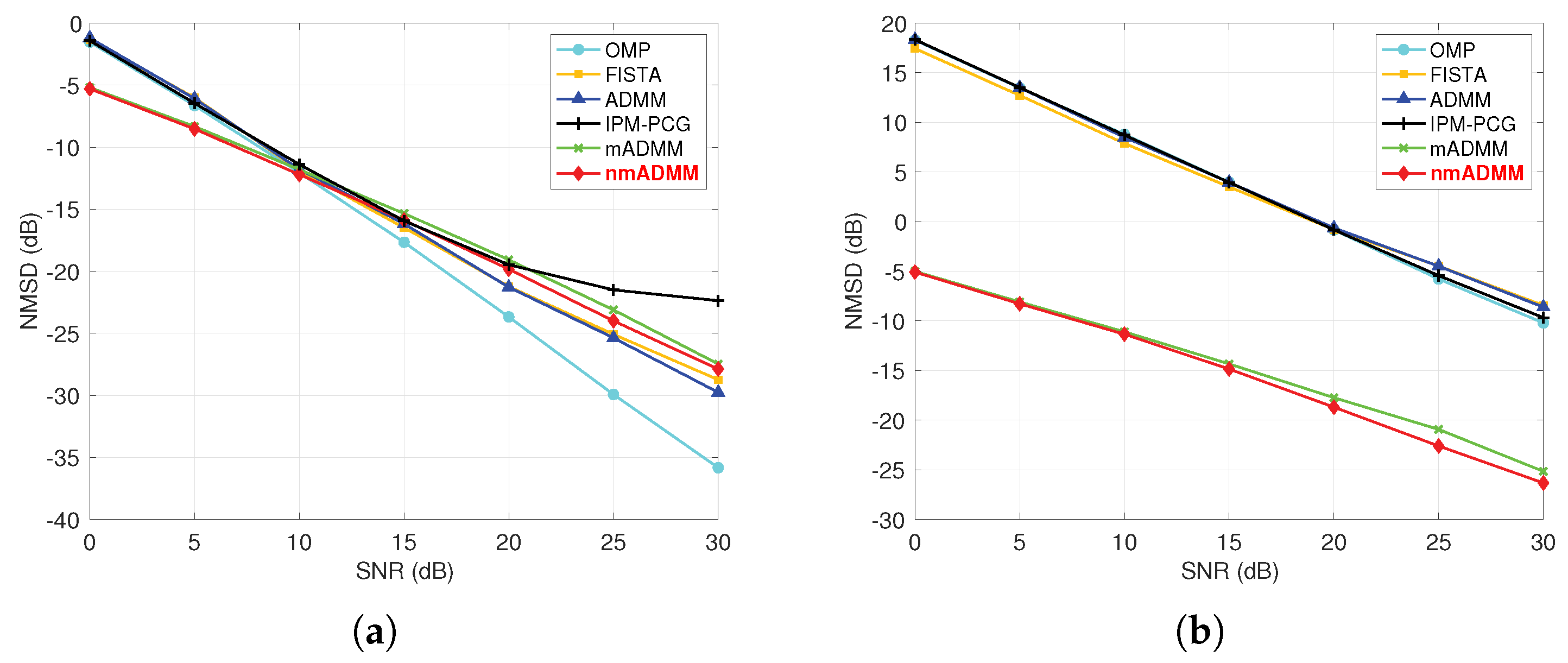
4.1. Simulation I: CIR Estimation in Single-Carrier System
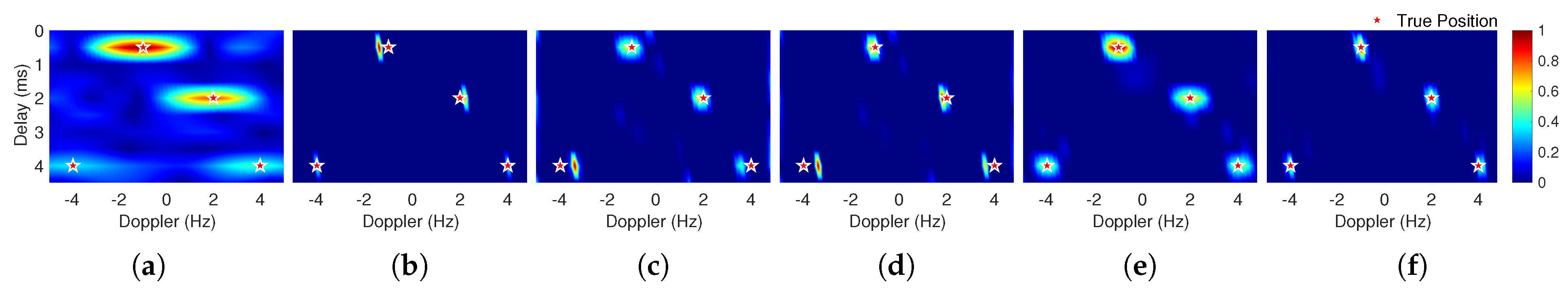
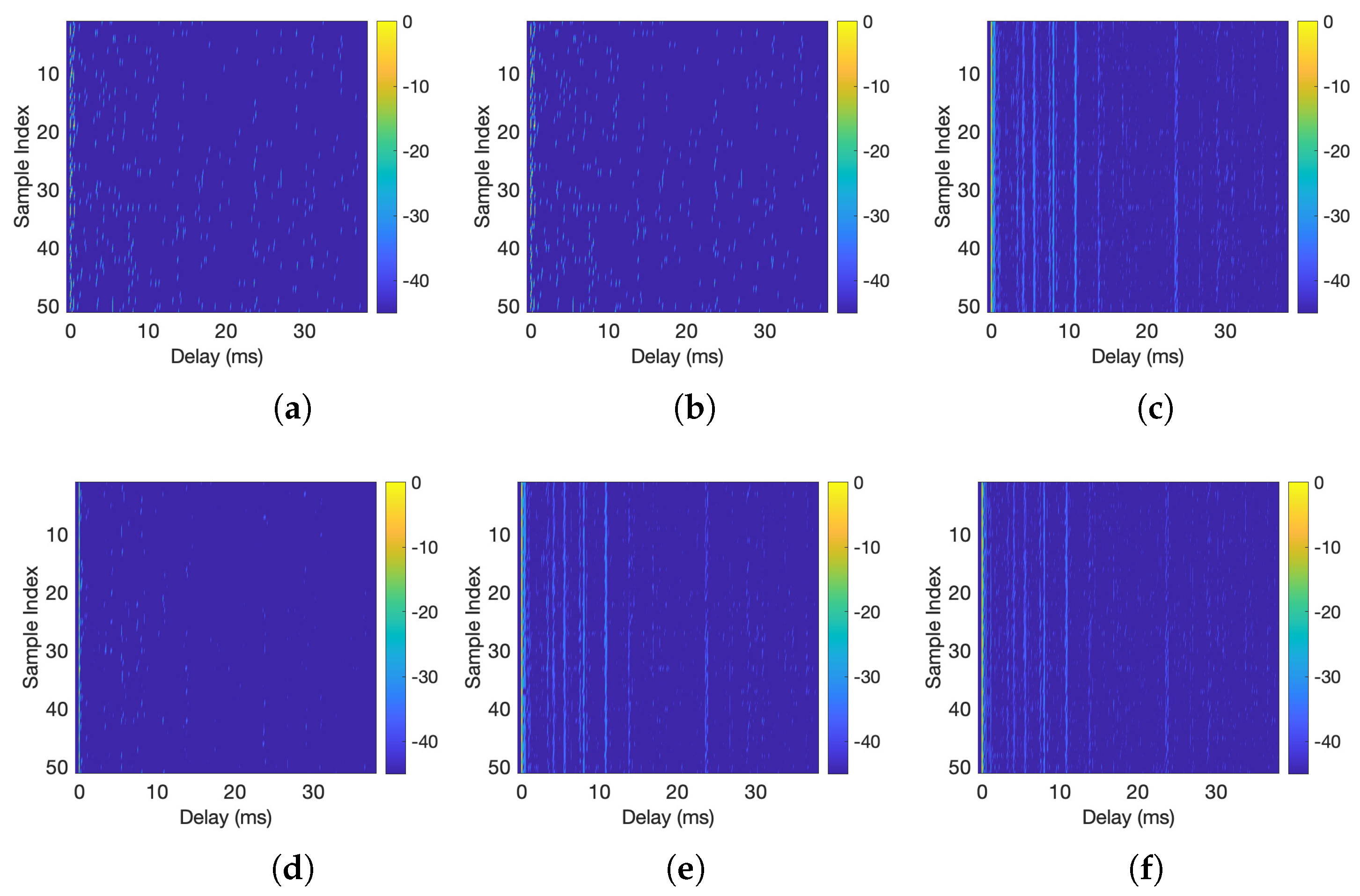
4.2. Simulation II: Doubly Spread Channel Estimation
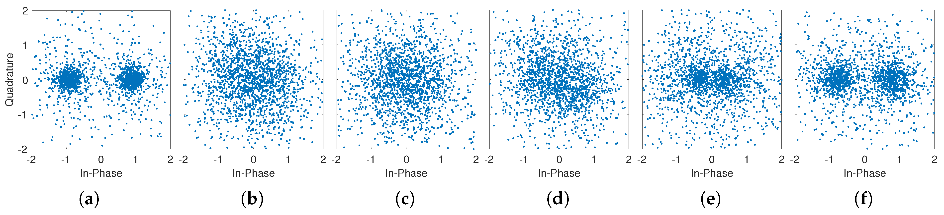
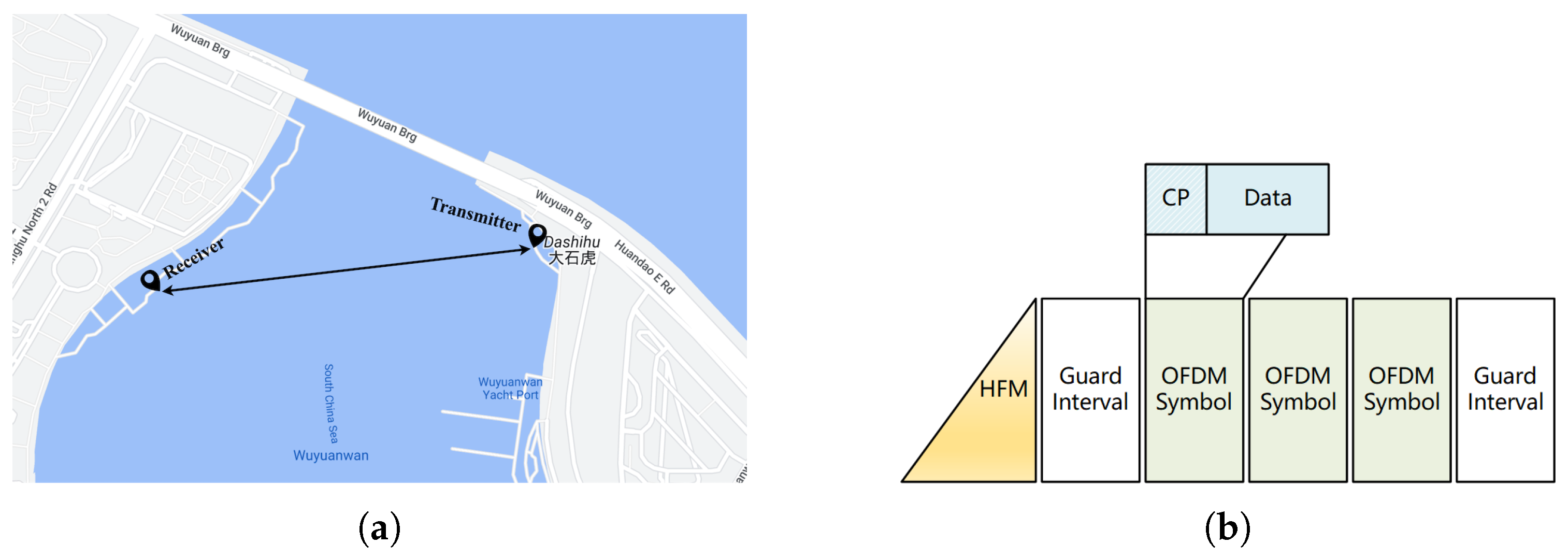
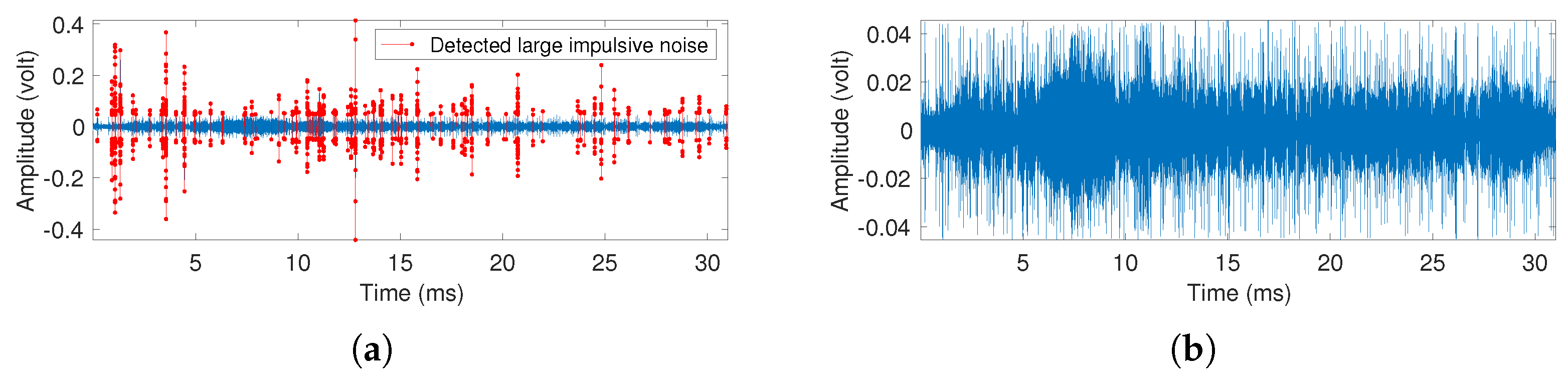
5. At-Sea Experiment
6. Conclusions
Author Contributions
Funding
Data Availability Statement
Acknowledgments
Conflicts of Interest
References
- Jahanbakht, M.; Xiang, W.; Hanzo, L.; Rahimi Azghadi, M. Internet of Underwater Things and Big Marine Data Analytics—A Comprehensive Survey. IEEE Commun. Surv. Tutor. 2021, 23, 904–956. [Google Scholar] [CrossRef]
- Zhou, Y.; Wang, R.; Yang, X.; Tong, F. Orthogonal Projection and Distributed Compressed Sensing-Based Impulsive Noise Estimation for Underwater Acoustic OSDM Communication. IEEE Internet Things J. 2023, 10, 22279–22293. [Google Scholar] [CrossRef]
- Bello, O.; Zeadally, S. Internet of Underwater Things Communication: Architecture, Technologies, Research Challenges and Future Opportunities. Ad Hoc Netw. 2022, 135, 102933. [Google Scholar] [CrossRef]
- Wei, X.; Guo, H.; Wang, X.; Wang, X.; Qiu, M. Reliable Data Collection Techniques in Underwater Wireless Sensor Networks: A Survey. IEEE Commun. Surv. Tutor. 2022, 24, 404–431. [Google Scholar] [CrossRef]
- Ouyang, D.; Li, Y.; Wang, Z. Channel Estimation for Underwater Acoustic OFDM Communications: An Image Super-Resolution Approach. In Proceedings of the ICC 2021—IEEE International Conference on Communications, Montreal, QC, Canada, 14–23 June 2021; pp. 1–6. [Google Scholar]
- Huang, S.H.; Tsao, J.; Yang, T.C.; Cheng, S.W. Model-Based Signal Subspace Channel Tracking for Correlated Underwater Acoustic Communication Channels. IEEE J. Ocean. Eng. 2014, 39, 343–356. [Google Scholar] [CrossRef]
- Wu, F.Y.; Tian, T.; Su, B.X.; Song, Y.C. Hadamard–Viterbi Joint Soft Decoding for MFSK Underwater Acoustic Communications. Remote Sens. 2022, 14, 6038. [Google Scholar] [CrossRef]
- Kaddouri, S.; Beaujean, P.P.J.; Bouvet, P.J.; Real, G. Least Square and Trended Doppler Estimation in Fading Channel for High-Frequency Underwater Acoustic Communications. IEEE J. Ocean. Eng. 2014, 39, 179–188. [Google Scholar] [CrossRef]
- Athaudage, C.; Jayalath, A. Enhanced MMSE Channel Estimation Using Timing Error Statistics for Wireless OFDM Systems. IEEE Trans. Broadcast. 2004, 50, 369–376. [Google Scholar] [CrossRef]
- Panayirci, E.; Altabbaa, M.T.; Uysal, M.; Poor, H.V. Sparse Channel Estimation for OFDM-Based Underwater Acoustic Systems in Rician Fading with a New OMP-MAP Algorithm. IEEE Trans. Signal Process. 2019, 67, 1550–1565. [Google Scholar] [CrossRef]
- Wu, F.Y.; Yang, K.; Tong, F.; Tian, T. Compressed Sensing of Delay and Doppler Spreading in Underwater Acoustic Channels. IEEE Access 2018, 6, 36031–36038. [Google Scholar] [CrossRef]
- Li, W.; Preisig, J.C. Estimation of Rapidly Time-Varying Sparse Channels. IEEE J. Ocean. Eng. 2007, 32, 927–939. [Google Scholar] [CrossRef]
- Sun, Q.; Wu, F.Y.; Yang, K.; Ma, Y. Estimation of Multipath Delay-Doppler Parameters from Moving LFM Signals in Shallow Water. Ocean Eng. 2021, 232, 109125. [Google Scholar] [CrossRef]
- Wang, Z.; Li, Y.; Wang, C.; Ouyang, D.; Huang, Y. A-OMP: An Adaptive OMP Algorithm for Underwater Acoustic OFDM Channel Estimation. IEEE Wirel. Commun. Lett. 2021, 10, 1761–1765. [Google Scholar] [CrossRef]
- Cai, T.T.; Wang, L. Orthogonal Matching Pursuit for Sparse Signal Recovery With Noise. IEEE Trans. Inf. Theory 2011, 57, 4680–4688. [Google Scholar] [CrossRef]
- Wu, F.Y.; Song, Y.C.; Yang, K. An Effective Framework for Underwater Acoustic Data Acquisition. Appl. Acoust. 2021, 182, 108235. [Google Scholar] [CrossRef]
- Donoho, D.L.; Tsaig, Y.; Drori, I.; Starck, J.L. Sparse Solution of Underdetermined Systems of Linear Equations by Stagewise Orthogonal Matching Pursuit. IEEE Trans. Inf. Theory 2012, 58, 1094–1121. [Google Scholar] [CrossRef]
- Fletcher, A.K.; Rangan, S.; Goyal, V.K. Necessary and Sufficient Conditions for Sparsity Pattern Recovery. IEEE Trans. Inf. Theory 2009, 55, 5758–5772. [Google Scholar] [CrossRef]
- Ben-Haim, Z.; Eldar, Y.C.; Elad, M. Coherence-Based Performance Guarantees for Estimating a Sparse Vector under Random Noise. IEEE Trans. Signal Process. 2010, 58, 5030–5043. [Google Scholar] [CrossRef]
- Berger, C.R.; Zhou, S.; Preisig, J.C.; Willett, P. Sparse Channel Estimation for Multicarrier Underwater Acoustic Communication: From Subspace Methods to Compressed Sensing. IEEE Trans. Signal Process. 2010, 58, 1708–1721. [Google Scholar] [CrossRef]
- Kim, S.J.; Koh, K.; Lustig, M.; Boyd, S.; Gorinevsky, D. An Interior-Point Method for Large-Scale-Regularized Least Squares. IEEE J. Sel. Top. Signal Process. 2007, 1, 606–617. [Google Scholar] [CrossRef]
- Zheng, P.; Lyu, X.; Gong, Y. Trainable Proximal Gradient Descent-Based Channel Estimation for mmWave Massive MIMO Systems. IEEE Wirel. Commun. Lett. 2023, 12, 1781–1785. [Google Scholar] [CrossRef]
- Beck, A.; Teboulle, M. A Fast Iterative Shrinkage-Thresholding Algorithm for Linear Inverse Problems. SIAM J. Imaging Sci. 2009, 2, 183–202. [Google Scholar] [CrossRef]
- Liu, H.; Zhang, J.; Wu, Q.; Xiao, H.; Ai, B. ADMM Based Channel Estimation for RISs Aided Millimeter Wave Communications. IEEE Commun. Lett. 2021, 25, 2894–2898. [Google Scholar] [CrossRef]
- Boyd, S. Distributed Optimization and Statistical Learning via the Alternating Direction Method of Multipliers. Found. Trends Mach. Learn. 2010, 3, 1–122. [Google Scholar] [CrossRef]
- Khan, M.R.; Das, B.; Pati, B.B. Channel Estimation Strategies for Underwater Acoustic (UWA) Communication: An Overview. J. Frankl. Inst. 2020, 357, 7229–7265. [Google Scholar] [CrossRef]
- Kuai, X.; Sun, H.; Zhou, S.; Cheng, E. Impulsive Noise Mitigation in Underwater Acoustic OFDM Systems. IEEE Trans. Veh. Technol. 2016, 65, 8190–8202. [Google Scholar] [CrossRef]
- Tian, T.; Raj, A.; Xavier, B.M.; Zhang, Y.; Wu, F.Y.; Yang, K. A Robust ADMM-Based Optimization Algorithm For Underwater Acoustic Channel Estimation. In Proceedings of the OCEANS 2023—Limerick IEEE Conference, Limerick, Ireland, 5–8 June 2023; pp. 1–5. [Google Scholar]
- Ye, H.; Li, G.Y.; Juang, B.H. Power of Deep Learning for Channel Estimation and Signal Detection in OFDM Systems. IEEE Wirel. Commun. Lett. 2018, 7, 114–117. [Google Scholar] [CrossRef]
- Jiang, R.; Wang, X.; Cao, S.; Zhao, J.; Li, X. Deep Neural Networks for Channel Estimation in Underwater Acoustic OFDM Systems. IEEE Access 2019, 7, 23579–23594. [Google Scholar] [CrossRef]
- Liu, L.; Cai, L.; Ma, L.; Qiao, G. Channel State Information Prediction for Adaptive Underwater Acoustic Downlink OFDMA System: Deep Neural Networks Based Approach. IEEE Trans. Veh. Technol. 2021, 70, 9063–9076. [Google Scholar] [CrossRef]
- Lv, X.; Li, Y.; Wu, Y.; Wang, X.; Liang, H. Joint Channel Estimation and Impulsive Noise Mitigation Method for OFDM Systems Using Sparse Bayesian Learning. IEEE Access 2019, 7, 74500–74510. [Google Scholar] [CrossRef]
- Chen, P.; Rong, Y.; Nordholm, S.; He, Z. Joint Channel and Impulsive Noise Estimation in Underwater Acoustic OFDM Systems. IEEE Trans. Veh. Technol. 2017, 66, 10567–10571. [Google Scholar] [CrossRef]
- Lee, J.; Park, C.; Ryu, E. A Geometric Structure of Acceleration and Its Role in Making Gradients Small Fast. Neural Inf. Process. Syst. 2021, 34, 11999–12012. [Google Scholar]
- Zhang, Y.; Venkatesan, R.; Dobre, O.A.; Li, C. Efficient Estimation and Prediction for Sparse Time-Varying Underwater Acoustic Channels. IEEE J. Ocean. Eng. 2020, 45, 1112–1125. [Google Scholar] [CrossRef]
- Parikh, N.; Boyd, S. Proximal Algorithms. Found. Trends Optim. 2014, 1, 127–239. [Google Scholar] [CrossRef]
- Wen, F.; Liu, P.; Liu, Y.; Qiu, R.C.; Yu, W. Robust Sparse Recovery in Impulsive Noise via ℓp-ℓ1 Optimization. IEEE Trans. Signal Process. 2017, 65, 105–118. [Google Scholar] [CrossRef]
- Borsic, A.; Adler, A. A Primal–Dual Interior-Point Framework for Using the L1 or L2 Norm on the Data and Regularization Terms of Inverse Problems. Inverse Probl. 2012, 28, 095011. [Google Scholar] [CrossRef]
- Wang, S.; Liu, Q.; Xia, Y.; Dong, P.; Luo, J.; Huang, Q.; Feng, D.D. Dictionary Learning Based Impulse Noise Removal via L1–L1 Minimization. Signal Process. 2013, 93, 2696–2708. [Google Scholar] [CrossRef]
- Jiang, J.; Wang, Z.; Chen, C.; Lu, T. L1-L1 Norms for Face Super-Resolution with Mixed Gaussian-impulse Noise. In Proceedings of the 41st IEEE International Conference on Acoustics, Speech and Signal Processing (ICASSP 2016), Shanghai, China, 20–25 March 2016; pp. 2089–2093. [Google Scholar]
- Zhang, H.; Hager, W.W. A Nonmonotone Line Search Technique and Its Application to Unconstrained Optimization. SIAM J. Optim. 2004, 14, 1043–1056. [Google Scholar] [CrossRef]
- Li, H.; Lin, Z. Accelerated Proximal Gradient Methods for Nonconvex Programming. In Proceedings of the Advances in Neural Information Processing Systems 28 (NIPS 2015), Montréal, QC, Canada, 7–12 December 2015; Volume 28. [Google Scholar]
- Zhou, S.; Wang, Z. OFDM for Underwater Acoustic Communications; Wiley: Hoboken, NJ, USA, 2014. [Google Scholar]
- Zeng, W.J.; Xu, W. Fast Estimation of Sparse Doubly Spread Acoustic Channels. J. Acoust. Soc. Amer. 2012, 131, 303–317. [Google Scholar] [CrossRef]
- Emadi, M.; Miandji, E.; Unger, J. A Performance Guarantee for Orthogonal Matching Pursuit Using Mutual Coherence. Circuits Syst. Signal Process. 2018, 37, 1562–1574. [Google Scholar] [CrossRef]
- Donoho, D.L.; Elad, M. Optimally Sparse Representation in General (Nonorthogonal) Dictionaries via ℓ1 Minimization. Proc. Natl. Acad. Sci. USA 2003, 100, 2197–2202. [Google Scholar] [CrossRef]
- Li, B.; Zhou, S.; Stojanovic, M.; Freitag, L.; Willett, P. Multicarrier Communication Over Underwater Acoustic Channels with Nonuniform Doppler Shifts. IEEE J. Ocean. Eng. 2008, 33, 198–209. [Google Scholar]
- Jia, S.; Zou, S.; Zhang, X.; Da, L. Underwater Acoustic Channel Estimation Based on Sparse Bayesian Learning Algorithm. IEEE Access 2023, 11, 7829–7836. [Google Scholar] [CrossRef]


| Method | # Iter. | Runtime (s) | NMSD (dB) |
|---|---|---|---|
| OMP [15] | 64/64 | 0.32/0.32 | −12.05/8.85 |
| FISTA [23] | 43/40 | 0.11/0.17 | −11.89/7.85 |
| ADMM [25] | 35/23 | 0.12/0.11 | −11.83/8.45 |
| IPM-PCG [21] | 24/21 | 11.86/24.66 | −11.48/8.67 |
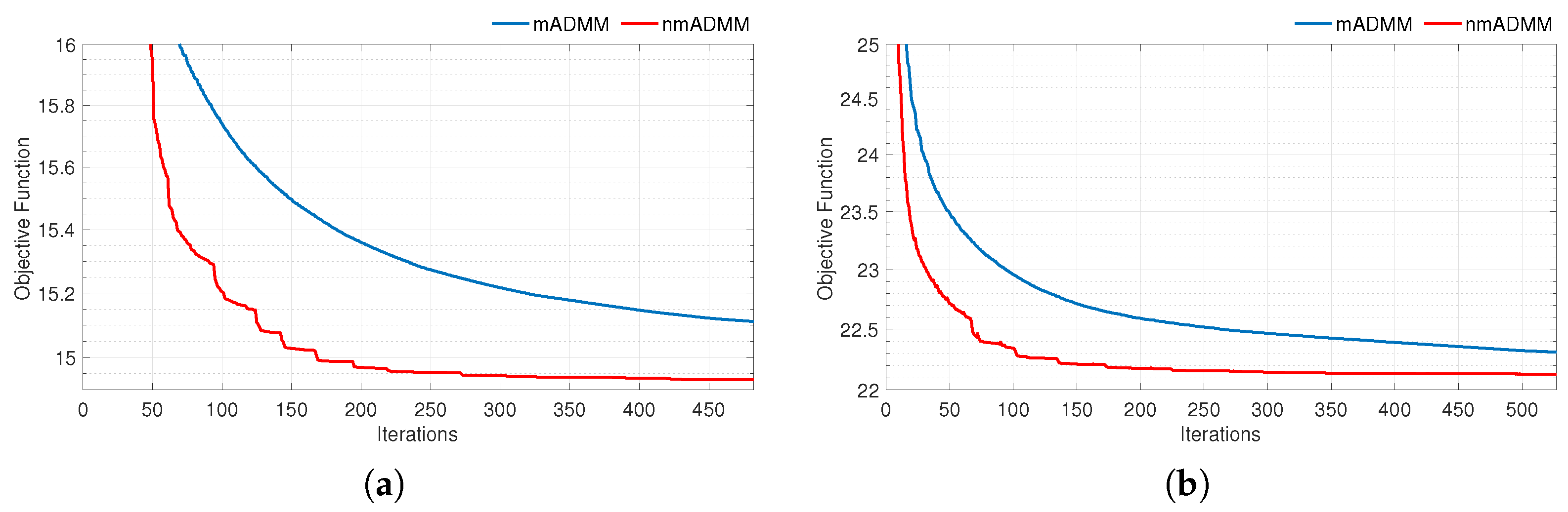
| mADMM [28] | 54/57 | 0.23/0.25 | −12.20/−11.25 |
| nmADMM | 43/42 | 0.31/0.33 | −12.22/−11.49 |
| Path No. | 1 | 2 | 3 | 4 |
|---|---|---|---|---|
| Delays (ms) | 0.5 | 2 | 4 | 4 |
| Doppler shift (Hz) | −1 | 2 | −4 | 4 |
| Modulus of amplitude | 1 | 0.8 | 0.5 | 0.5 |
| Method | # Iter. | Runtime (s) | # Err. | BER (%) |
|---|---|---|---|---|
| Ground Truth | -/- | -/- | 0/179 | 0/8.75 |
| OMP [15] | 4/4 | 0.004/0.004 | 179/791 | 8.95/39.55 |
| FISTA [23] | 564/835 | 1.16/1.54 | 9/729 | 0.45/36.45 |
| ADMM [25] | 662/610 | 0.51/0.63 | 0/619 | 0/30.95 |
| mADMM [28] | 1577/2193 | 5.85/7.89 | 557/547 | 27.85/27.35 |
| nmADMM | 481/527 | 3.15/3.51 | 0/252 | 0/12.60 |
| INR = 15 dB | INR = 25 dB | |||||
|---|---|---|---|---|---|---|
| q | 0.01 | 0.005 | 0.001 | 0.01 | 0.005 | 0.001 |
| Ground Truth | 2.10 | 0.80 | 0.30 | 18.80 | 8.85 | 2.50 |
| OMP [15] | 36.25 | 34.95 | 10.25 | 48.60 | 47.20 | 35.85 |
| FISTA [23] | 27.85 | 11.65 | 0.50 | 55.35 | 45.80 | 8.35 |
| ADMM [25] | 27.65 | 13.55 | 0.55 | 55.25 | 42.85 | 8.10 |
| mADMM [28] | 5.70 | 4.30 | 3.35 | 23.90 | 15.15 | 8.30 |
| nmADMM | 5.25 | 2.05 | 0.45 | 22.15 | 13.50 | 3.85 |
| Method | # Iter. | Runtime (s) | SER (%) |
|---|---|---|---|
| OMP [15] | 74 | 0.3152 | 10.68 |
| A-OMP [14] | 85 | 0.56 | 7.45 |
| FISTA [23] | 24 | 1.0852 | 5.87 |
| FM-SBL [48] | 57 | 9.73 | 5.83 |
| ADMM [25] | 47 | 13.1543 | 6.61 |
| nmADMM | 32 | 1.4681 | 4.48 |
Disclaimer/Publisher’s Note: The statements, opinions and data contained in all publications are solely those of the individual author(s) and contributor(s) and not of MDPI and/or the editor(s). MDPI and/or the editor(s) disclaim responsibility for any injury to people or property resulting from any ideas, methods, instructions or products referred to in the content. |
© 2024 by the authors. Licensee MDPI, Basel, Switzerland. This article is an open access article distributed under the terms and conditions of the Creative Commons Attribution (CC BY) license (https://creativecommons.org/licenses/by/4.0/).
Share and Cite
Tian, T.; Yang, K.; Wu, F.-Y.; Zhang, Y. Channel Estimation for Underwater Acoustic Communications in Impulsive Noise Environments: A Sparse, Robust, and Efficient Alternating Direction Method of Multipliers-Based Approach. Remote Sens. 2024, 16, 1380. https://doi.org/10.3390/rs16081380
Tian T, Yang K, Wu F-Y, Zhang Y. Channel Estimation for Underwater Acoustic Communications in Impulsive Noise Environments: A Sparse, Robust, and Efficient Alternating Direction Method of Multipliers-Based Approach. Remote Sensing. 2024; 16(8):1380. https://doi.org/10.3390/rs16081380
Chicago/Turabian StyleTian, Tian, Kunde Yang, Fei-Yun Wu, and Ying Zhang. 2024. "Channel Estimation for Underwater Acoustic Communications in Impulsive Noise Environments: A Sparse, Robust, and Efficient Alternating Direction Method of Multipliers-Based Approach" Remote Sensing 16, no. 8: 1380. https://doi.org/10.3390/rs16081380
APA StyleTian, T., Yang, K., Wu, F.-Y., & Zhang, Y. (2024). Channel Estimation for Underwater Acoustic Communications in Impulsive Noise Environments: A Sparse, Robust, and Efficient Alternating Direction Method of Multipliers-Based Approach. Remote Sensing, 16(8), 1380. https://doi.org/10.3390/rs16081380