A Deep Learning Localization Method for Acoustic Source via Improved Input Features and Network Structure

Abstract

Shallow water passive source localization is an essential problem in underwater detection and localization. Traditional matched-field processing (MFP) methods are sensitive to environment mismatches. Many neural network localization methods still have room for improvement in accuracy if they are further adjusted to underwater acoustic characteristics. To address these problems, we propose a deep learning localization method via improved input features and network structure, which can effectively estimate the depth and the closest point of approach (CPA) range of the acoustic source. Firstly, we put forward a feature preprocessing scheme to enhance the localization accuracy and robustness. Secondly, we design a deep learning network structure to improve the localization accuracy further. Finally, we propose a method of visualizing the network to optimize the estimated localization results. Simulations show that the accuracy of the proposed method is better than other compared features and network structures, and the robustness is significantly better than that of the MFP methods. Experimental results further prove the effectiveness of the proposed method.

1. Introduction

Passive source localization in shallow water has always been an essential problem in underwater acoustic detection and localization [1,2]. The matched-field processing (MFP) methods constitute the most common methods, which utilize the acoustic propagation model to generate the replica field and then match it with the measured field to obtain a two-dimensional ambiguity plane whose peaks indicate the source localization [3,4]. An incoherent matched-field processor can effectively enhance the main lobe ratio and improve localization performance when extending single-frequency MFP methods to multifrequency MFP methods [5,6]. Furthermore, the matched-phase coherent processor has been proven to be superior than the incoherent matched-field processor when there is a mismatch between the environment and variations in noise levels [7,8]. Gregory J. Orris et al. [9] proposed a magnitude crossfrequency processor, which reduced the side lobe more effectively than the conventional matched-phase coherent processor. Chen et al. [10] proposed a matched-phase coherent processor based on the phase descent search, which achieved lower complexity than the simulated annealing algorithm while possessing high localization accuracy. However, there are two major unavoidable drawbacks with respect to the existing MFP methods. First, the localization performance is heavily dependent on the environment parameters and has limited resistance to environment mismatches, thus making the MFP methods difficult to apply in the complex ocean environment [11,12]. Second, the improved algorithms usually require a large amount of running time [13].

In recent years, the artificial intelligence (AI) localization methods have gradually gained importance [14,15,16]. In underwater source localization, unlike the MFP methods that utilize sound propagation models, AI methods are data-driven and directly learn the relationship between input features and source position through powerful nonlinear fitting capabilities [17,18]. Neural networks are widely used models in AI and have been employed in various localization scenarios to achieve higher accuracy in localization and stronger resistance against environment mismatches compared to the MFP methods [19,20]. Niu et al. [21] used a feedforward neural network to estimate the horizontal distance between a target and a vertical linear array (VLA) in shallow water, thus surpassing the accuracy of the MFP methods in simulations and the Noise09 experiment. Zhu et al. [22] used a two-step semisupervised framework for underwater source localization, and they proposed an interpretable feature selection method based on principal component regression (PCR) to accelerate the training stage operation time in the SWellEx-96 experiment. T.B. Neilsen et al. [23] used a convolutional neural network of multitask learning (CNN-MTL) to estimate parameters such as distance, velocity, and seabed type of a moving target simultaneously. The SBCEX 2017 experiment verified the ability of CNN-MTL by using a 75 min midfrequency source.

With the rapid development of computer arithmetic power, deep learning has become the mainstream trend for a variety of research fields, especially in signal processing such as images and speech [24]. In recent years, it has also been used in underwater acoustic localization [25,26]. Niu et al. [27] used ResNet50 in a shallow water environment to estimate the depth and range of a multifrequency source by using the source magnitude. The method obtained better localization performance than SAGA (a software package for MFP), which has been verified in the 2011 Yellow Sea experiment. Huang et al. [28] used a time delay neural network (TDNN) and a convolutional and deep neural network (CNN-DNN) to estimate the depth and the range of a wideband source. The network trained on the simulation data achieved a fairly good performance on the 1999 Yellow Sea experiment, which estimated a near-surface vessel at a distance of 12 km. However, many researchers directly apply the classical feature processing schemes and deep network structures to underwater acoustic localization problems without making sufficient improvements based on underwater acoustic characteristics. On the one hand, the underwater acoustic features make it more difficult to establish mapping relationships than traditional image and speech features. If the classical feature scheme and network structure are used directly, the localization accuracy may not be high enough. Therefore, it is necessary to design the input features and the network structure based on the underwater acoustic scene [29]. On the other hand, the ability of deep learning method depends on the quantity and diversity of training samples, but ensuring that the underwater acoustic data meet such requirements is difficult. The challenge lies in obtaining a deep learning method with strong robustness [30].

To address the shortcomings of the existing localization methods, we propose a deep learning localization method via improved input features and network structure. The proposed method can estimate the depth and the closest point of approach (CPA) range of an acoustic source, and it excels in achieving high accuracy and robustness in shallow water passive source localization problems. The main contributions of the proposed method are summarized in the following three aspects:

• A feature preprocessing scheme is proposed. To improve the localization accuracy, the feature processing step creates the multitime pressure and eigenvector feature (MTPEF). To enhance the localization robustness, the feature augmentation step expands the training datasets in environment parameters and target motion parameters.
• An inception and residual in-series network (IRSNet) is designed. To further improve the localization accuracy, the main module IRS concatenates inception modules and residual modules in the series, and the number of network parameters has been adjusted to account for the acoustic source localization problem.
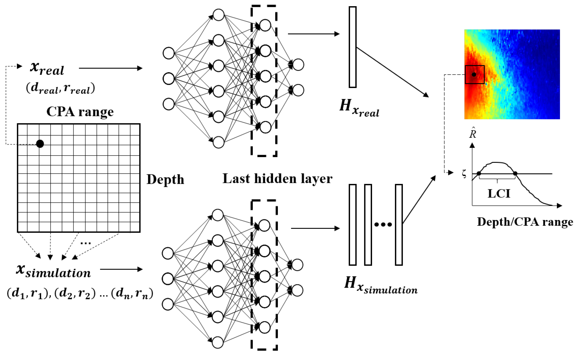
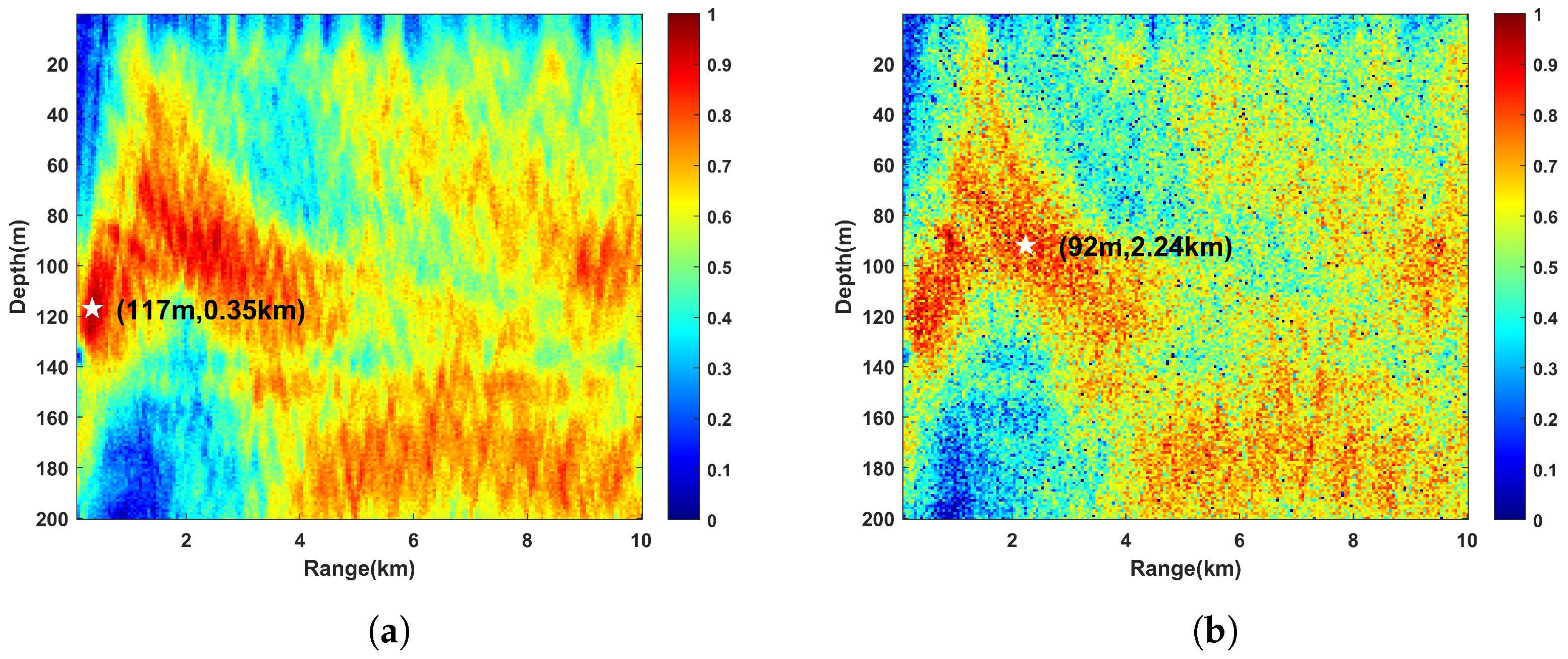
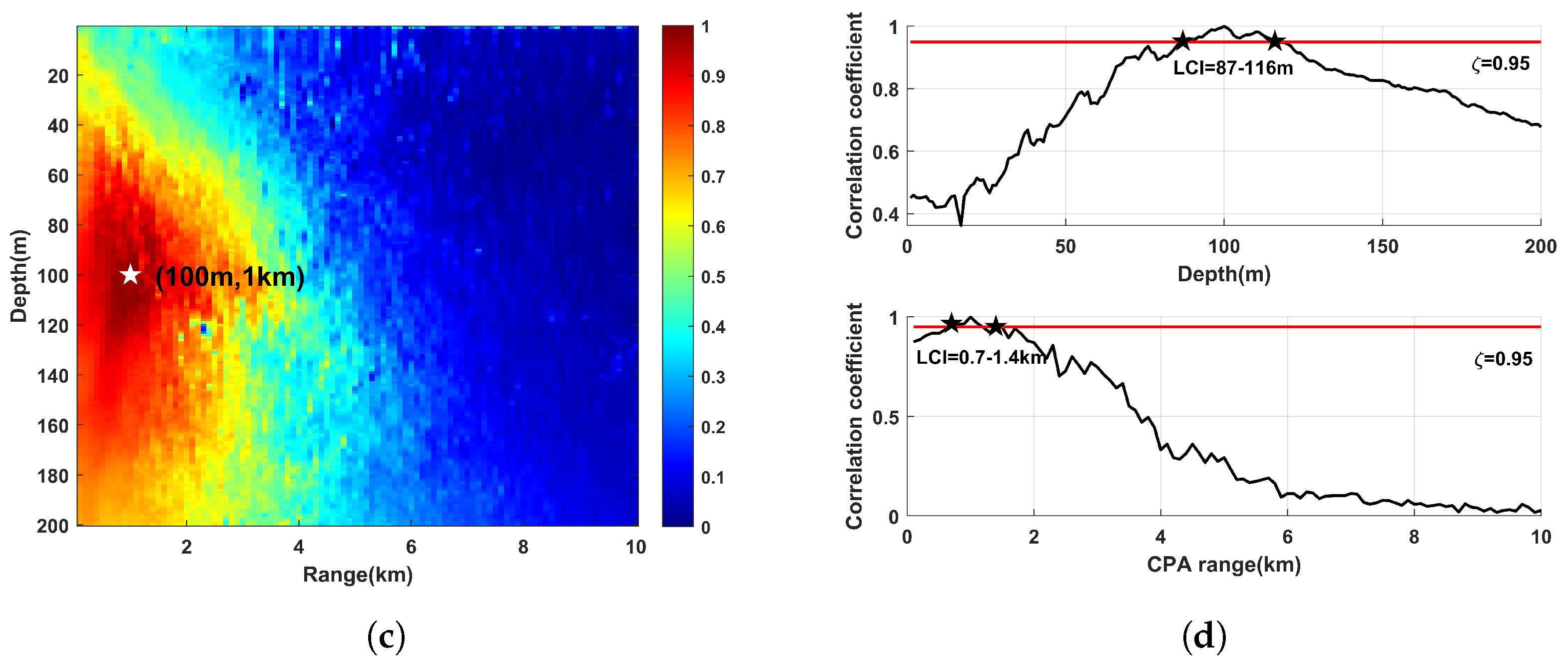
• A visualization method of the network is presented using hidden layer features. To optimize the estimated localization results, the localization confidence interval (LCI) is defined using the visualization method and can obtain the source position interval of high confidence.

The simulation and experimental results have shown that the proposed method has better localization accuracy compared to three other features and ten network structures, and significantly improves the localization robustness compared to the improved MFP methods when there is a mismatch in the environment. Additionally, the visualization method further provides high confidence localization intervals. The capability of the proposed method has been further verified by the SWellEx-96 experiment.

The rest of the paper is organized as follows. Section 2 describes the materials and methods of the proposed method. Section 3 shows the simulation and experimental results. Section 4 introduces the discussion of the method. Section 5 summarizes the paper.

2. Materials and Methods

2.1. Features Preprocessing Module Design

In this section, we design a feature preprocessing scheme that includes feature processing and feature augmentation. Firstly, we design a composite input feature MTPEF in the feature processing step. It is preprocessed from the raw time domain signals received using VLAs, which can improve the localization accuracy. Secondly, we expand the training datasets in the feature augmentation step. It can enhance the robustness of environment parameters and target motion parameters.

2.1.1. Conventional Features

Consider a single acoustic source with several line spectrums; the signal is received by the VLA. The complex pressure at frequency f obtained by array element l can be modeled as a combination of the source term s and noise $\epsilon$

$$p_l\left(f\right)=s(f,l,\mu ,\eta )+\epsilon .$$

(1)

In Equation (1), $\mu$ represents the set of target information (distance, depth, etc.). $\eta$ represents the set of environment parameters and target motion parameters. At every sampling time, the signal with F frequency points received by L element VLAs can be processed as F×L dimensional complex pressures:

$$\mathit{P}=\left[\begin{array}{cccc}{p}_1\left(f_1\right)& p_2\left(f_1\right)& \cdots & p_L\left(f_1\right)\\ p_1\left(f_2\right)& p_2\left(f_2\right)& \cdots & p_L\left(f_2\right)\\ ⋮& ⋮& \ddots & ⋮\\ p_1\left(F\right)& p_2\left(F\right)& \cdots & p_L\left(F\right)\end{array}\right]=\left[\begin{array}{c}\mathit{p}\left(f_1\right)\\ \mathit{p}\left(f_2\right)\\ ⋮\\ \mathit{p}\left(F\right)\end{array}\right].$$

(2)

The input features for localization should reduce the effect of source amplitude, so the complex pressures are always normalized, and the normalized sample covariance matrices (SCMs) form the conjugate symmetric matrix [21]:

$$\widehat{\mathit{p}}\left(f\right)=\frac{\mathit{p}\left(f\right)}{{∥\mathit{p}\left(f\right)∥}_2}=\frac{\mathit{p}\left(f\right)}{\sqrt{{\sum }_{l=1}^L{\left|p_l\left(f\right)\right|}^2}}.$$

(3)

$$\mathit{C}\left(\mathit{f}\right)=\widehat{\mathit{p}}{\left(f\right)}^{+}\widehat{\mathit{p}}\left(f\right).$$

(4)

In Equation (4), ${\left(·\right)}^{+}$ stands for Hermitian transpose, and the matrix $\mathit{C}\left(f\right)$ reflects the amplitude and phase difference of sound pressure between each element, but it also contains noise and interference information. Eigenvalue decomposition can effectively retain the critical information [28].

$$\begin{array}{cc}\hfill \mathit{C}\left(f\right)& ={{\mathsf{\Lambda }}_f}^{+}{\mathsf{\Sigma }}_f{\mathsf{\Lambda }}_f\hfill \\ \hfill & ={\left[\begin{array}{c}{\mathit{e}}_{f1}\\ {\mathit{e}}_{f2}\\ ⋮\\ {\mathit{e}}_{fL}\end{array}\right]}^{+}\left[\begin{array}{cccc}{\lambda }_{f1}& 0& \cdots & 0\\ 0& {\lambda }_{f2}& \cdots & 0\\ ⋮& ⋮& \ddots & ⋮\\ 0& 0& \cdots & {\lambda }_{fL}\end{array}\right]\left[\begin{array}{c}{\mathit{e}}_{f1}\\ {\mathit{e}}_{f2}\\ ⋮\\ {\mathit{e}}_{fL}\end{array}\right]\hfill \end{array}.$$

(5)

In Equation (5), ${\mathsf{\Sigma }}_f$ represents the eigenvalue diagonal matrix, and ${\lambda }_{f1}\ge {\lambda }_{f2}\ge \cdots \ge {\lambda }_{fL}$. ${\mathsf{\Sigma }}_f$ represents the eigenvector. For a single source, the eigenvector ${\mathit{e}}_{f1}$ corresponding to the largest eigenvalue ${\lambda }_{f1}$ contains the most signal information.

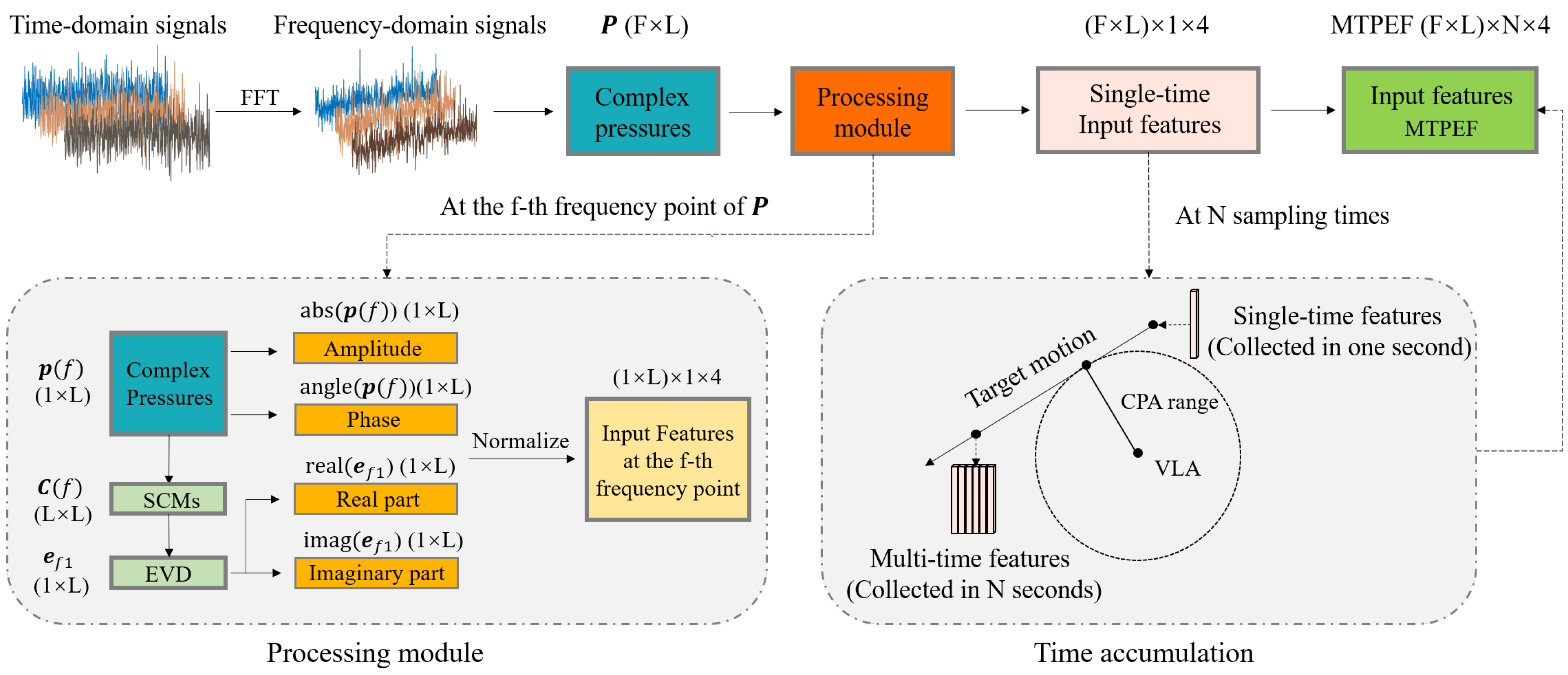
2.1.2. Features Processing

Based on the above feature processing methods, we proposed the MTPEF as an input feature. The design of the MTPEF includes the following two parts [31]:

• We used complex pressure and eigenvector features at each sampling time as single-time input features. The complex pressure features are general features without complex preprocessing and retain much of the original information. The eigenvector features are specific features created by the SCMs using eigenvalue decomposition. They consume some original information but can better represent the nonlinear mapping relationship. When using the deep learning model, combining general and specific features often performs better than the features used alone.
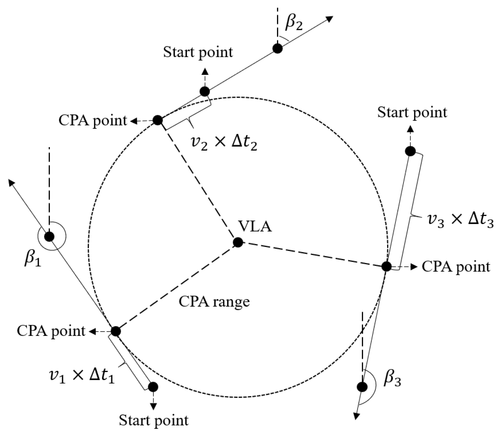
• We extended the single-time features to multitime features. In general, as the source moves for a period of time, the depth can be regarded as a constant, and the distance between the VLA and the source will change. The CPA range is a constant in this process, which can replace the distance. For the depth and the CPA range, the extension of the time domain dimension is equivalent to increasing the original information, and it will make the nonlinear relationship mentioned in Equation (1) more stable to learn.

The overall feature processing step is shown in Figure 1. Firstly, Fast Fourier Transform (FFT) was used to obtain complex pressures from the raw time domain signals collected by VLA. Secondly, the complex pressures were converted to the SCMs by Equations (3) and (4), and then we reduced the dimension of the SCMs to obtain ${\mathit{e}}_{f1}$ by Equation (5). Finally, the composite features of each sampling time were normalized, and the MTPEF was formed by multiple normalization composite single-time features. In addition, the network model cannot directly take complex numbers as input features, so the MTPEF was composed of four parts at each frequency point: the complex pressures amplitude abs($\mathit{p}\left(f\right)$), the complex pressures phase($\mathit{p}\left(f\right)$), the real part of eigenvector features real(${\mathit{e}}_{f1}$), and the imaginary part imag(${\mathit{e}}_{f1}$). Assuming that the single acoustic source is in uniform linear motion; the L-element VLA can obtain (F × L) × N × 4 dimension input features from F frequency points at N sampling times. The estimators of the network are the depth and the CPA range, which are normalized as labels.

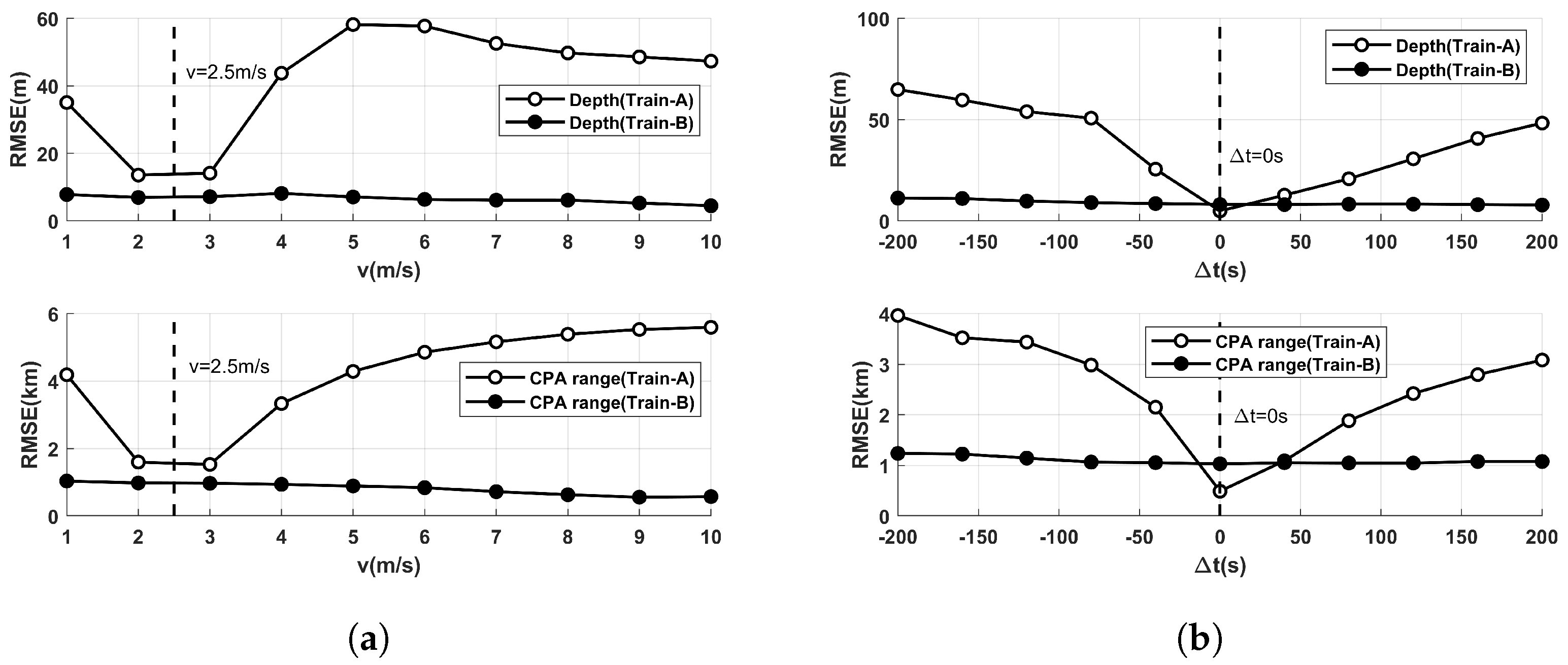
2.1.3. Features Augmentation

From the probabilistic standpoint, the network model learns the nonlinear relationship between $\mu$ and $p_l\left(f\right)$, in other words, the distribution of $P\left(\mu |p_l\left(f\right)\right)$ [32]. In Equation (1), $\eta$ can influence the distribution; therefore, training the network model in various $\eta$ cases of input features is an effective way to improve the robustness. The feature augmentation only needs to select parameters with a more significant impact, because not all parameters in $\eta$ impact the localization results. A sensitivity analysis of environmental parameters and location results has been studied. It has been verified in [27] that the water depth, the substrate thickness, and the sound velocity at the top of the substrate greatly impact the localization results.

On this basis, we analyzed the sensitivity of the target motion parameters. We assumed that the target motion trajectory is approximated as a certain tangent line on the circle centered at the location of the VLA and radiused at the CPA range. As shown in Figure 2, while maintaining the same depth and the CPA range, the target motion has various possibilities. Figure 3 gives the input features corresponding to various motion parameters when the simulation source position is the same (depth = 100 m and CPA range = 1 km); the simulation input features were built by using the parameters mentioned in Section 2.3.1. The following conclusions can be drawn about the sensitivity analysis of motion parameters:

• The input features almost did not change with the source course $\beta$, as can be seen by comparing Figure 3a and Figure 3b.
• The source velocity v changed; then, the visualized stripes of the input features changed accordingly, as can be seen by comparing Figure 3a and Figure 3c.
• The shape of the visualized stripes was almost unchanged, but an overall translation ensued with the change in the starting point of the target, as can be seen by comparing Figure 3a and Figure 3d.

In summary, the change in the source velocity v and the starting point greatly impacted the input features, which we need to further augment to enhance the robustness. Assuming that the starting point is at CPA time, the change in the starting point can be represented by the time difference $\Delta t$ between the starting point and the CPA time.

Figure 2. The overall feature processing flow of the MTPEF.

Figure 2. The overall feature processing flow of the MTPEF.

Figure 3. The simulation input feature maps in different target motion parameters: (a) $v=2.5$ m/s, $\Delta t=0$ s, $\beta ={30}^{\circ }$. (b) $v=2.5$ m/s, $\Delta t=0$ s, $\beta ={120}^{\circ }$. (c) $v=5$ m/s, $\Delta t=0$ s, $\beta ={30}^{\circ }$. (d) $v=2.5$ m/s, $\Delta t=-30$ s, $\beta ={30}^{\circ }$.

Figure 3. The simulation input feature maps in different target motion parameters: (a) $v=2.5$ m/s, $\Delta t=0$ s, $\beta ={30}^{\circ }$. (b) $v=2.5$ m/s, $\Delta t=0$ s, $\beta ={120}^{\circ }$. (c) $v=5$ m/s, $\Delta t=0$ s, $\beta ={30}^{\circ }$. (d) $v=2.5$ m/s, $\Delta t=-30$ s, $\beta ={30}^{\circ }$.

2.2. Deep Learning Network Design

In this section, we design a deep network structure IRSNet for underwater acoustic localization. The main module of the proposed network not only has the ability of the inception module to learn multiple scale features simultaneously but also has the ability of the residual module to inhibit overfitting. In addition, we propose a network visualization method and define the LCI to optimize the estimated localization results.

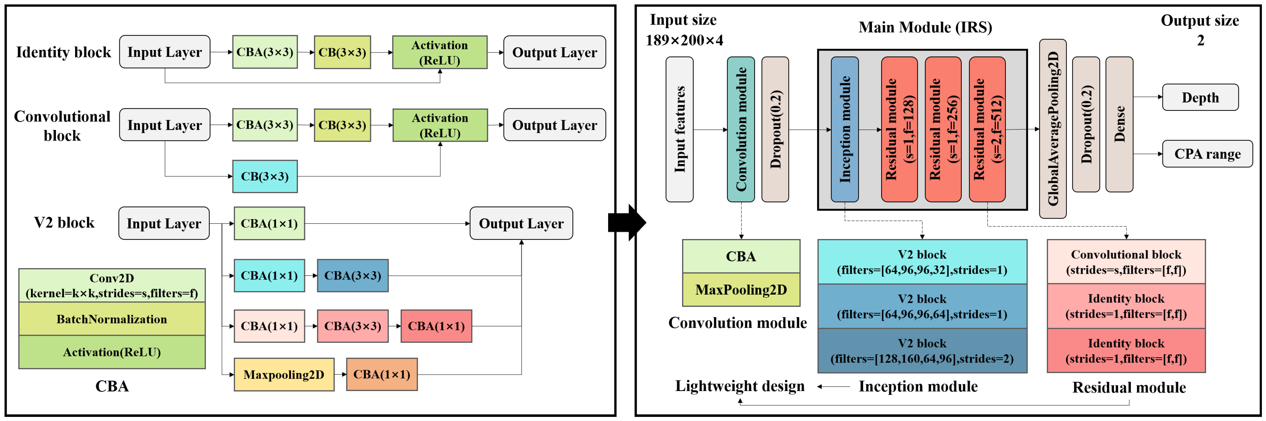
2.2.1. Residual Module and Inception Module

The convolutional structure is good at abstracting advanced features from simple edge information, and the essence is to use convolutional kernels as filters to multiply the input features to achieve edge detection, sharpening, and blurring. Therefore, convolutional neural networks are suitable for processing image features, including pseudo image features made by feature splicing [33]. Deep neural networks can capture richer semantic features than shallow neural networks. However, the increase in the number of layers of the network causes the critical information of the input features to be lost layer by layer, thus making the network more difficult to converge [34]. The residual module and the inception module are effective structures for solving the convergence problem of deep neural networks [35,36,37,38].

The residual module proposes a jump connection residual structure, which mitigates the information loss by learning the residuals of $x\to F\left(x\right)+x$ instead of the mapping relations of $x\to F\left(x\right)$. The residual structure can effectively suppress overfitting, and the deepening of layers will not cause the vanishing gradient problem, which will affect the performance of the network. The inception module proposes a multiscale convolutional kernel structure, which uses multiple convolutional kernels of different sizes in parallel at the same network level and utilizes convolutional kernels with varying fields of view to filter the same input features so that the critical information can be retained as much as possible.

However, the classical deep network structures based on these two modules are relatively complex, which not only dramatically increases the training time and the difficulty of training but also does not apply to such model complexity in some application scenarios. So, it is necessary to adjust the deep network structure according to the characteristics of the underwater acoustic localization problem.

2.2.2. Inception and Residual in Series Network

According to the characteristics of the underwater acoustic localization problem based on VLA, we designed a deep network structure IRSNet. The key points for designing the structure can be summarized as follows:

• The input features designed in Section 2.1 can be considered as image features that contain localization information for a period of time. To improve the understanding of features, the multiscale kernel was used to understand the information of different time and characteristic scales in input features. To prevent the abnormal degradation of network performance when deepening the layers, the structure of the residual module is the most suitable structure for suppressing overfitting.
• The complexity of the deep network structure should be appropriate: being too simple or too complex will affect network performance. To balance localization accuracy and training time, we carried out a lightweight design of the deep network structure and improved the training speed without losing the network localization accuracy.
• The IRS module was designed in series form rather than the nested form in [39]. This is because nested modules are very complex: the amount of training data for underwater acoustic localization problems makes it difficult to make the model converge.

Figure 4 presents the overall structure of the proposed IRSNet. The convolution module consists of the convolution, batch normalization, and activation (CBA) combination structure and max pooling structure. The main module IRS contains an improved inception module and residual module, which has been designed to be lightweight. The inception module consists of two V2 blocks with strides = 1 and one V2 block with strides = 2. The residual module can be decomposed into convolutional blocks and identity blocks. The global average pooling module replaces the average pooling module for rapid dimensionality reduction. The underwater acoustic localization can be regarded as a regression problem, and the output layer contains two neurons to estimate the depth and the CPA range. The activation function does not exist in the output layer.

2.2.3. Localization Confidence Interval for Visualization

Unlike the MFP methods, the neural network method gives localization results directly. But in a sense, the results are hard to trust because they do not show any calculation process. Although the calculation process of the neural network is a black box, there are also methods to prove that the network has learned the relationship between the input features and the label. It has been demonstrated in the study of convolutional neural network visualization that the features learned by the network close to the input layer are low-level features [40]. The features learned by the layers close to the output layer are discriminative vital features, which can reflect the mapping relationship between the input features and the quantity to be estimated.

In underwater acoustic localization, the crosscorrelation between the last hidden layer features, can prove the ability of the network. The grid points with a higher correlation value are more likely to correspond to the position of the measured source. The last hidden layer features are used to visualize the localization results of the network, and the visualization results can be regarded as a two-dimensional ambiguity plane similar to the MFP methods. The LCI is defined by setting a threshold for the visualization results. It is calculated by the formula

$$\left\{\begin{array}{c}\mathit{R}\left(m\right)=\frac{1}{N}{\sum }_{n=0}^{N-1}{\mathit{H}}_{x_{simulation}}\left(n\right){\mathit{H}}_{x_{real}}(n-m)\hfill \\ \widehat{\mathit{R}}=(\mathit{R}-min\left(\mathit{R}\right))/(max\left(\mathit{R}\right)-min\left(\mathit{R}\right))\hfill \\ \mathit{LCI}=\widehat{\mathit{R}}\left(find(\widehat{\mathit{R}}\ge \zeta )\right)\hfill \end{array}\right..$$

(6)

In (6), ${\mathit{H}}_{x_{simulation}}$ and ${\mathit{H}}_{x_{real}}$ represent the last hidden layer features for all the grid points and the measured source, respectively. $\mathit{R}\left(m\right)$ represents the crosscorrelation between the nth point of ${\mathit{H}}_{x_{simulation}}$ and the $(n-m)$th point of ${\mathit{H}}_{x_{simulation}}$. $\widehat{\mathit{R}}$ represents the normalized results of $\widehat{\mathit{R}}$. $\zeta$ represents the threshold.

The overall processing flow is shown in Figure 5. First, the measured source and the simulation source at grid points $\left(d_{real},r_{real}\right)$ and $\left(d_1,r_1\right),\left(d_2,r_2\right)\cdots \left(d_n,r_n\right)$ were preprocessed into input features $x_{real}$ and $x_{simulation}$. Second, the last hidden layer features were obtained through the trained network. Then, the visual localization results were obtained by the hidden features ${\mathit{H}}_{x_{real}}$ and ${\mathit{H}}_{x_{simulation}}$ via the crosscorrelation $\widehat{\mathit{R}}$. In addition, the region with a correlation value above the threshold $\zeta$ is defined as the LCI. It can give the localization interval with high confidence. If there is more than one region above the threshold, the envelope that has the largest correlation value will be taken as the LCI.

2.3. Experimental Settings

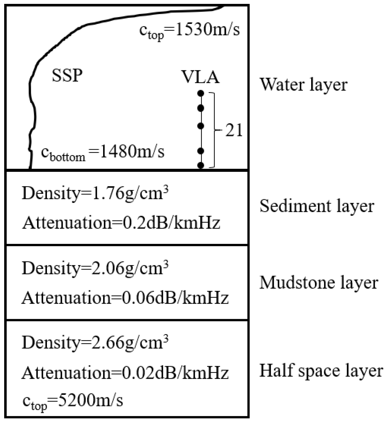
2.3.1. Simulation Datasets

In our experiments, we trained the neural network model on simulation datasets, which were built with reference to the SWellEx-96 experiment environment. The shallow waveguide environment was simulated with a seafloor substrate consisting of a sediment layer, a mudstone layer, and a fluid half space, as shown in Figure 6. The 21-element VLA covers the depth range of 94–216 m, and the spacing of the array elements is about 5.6 m. The frequency of the simulation source consists of several single frequency points, with the following nine specific values: 112 Hz, 130 Hz, 148 Hz, 166 Hz, 201 Hz, 235 Hz, 283 Hz, 338 Hz, and 388 Hz. The source motion duration was chosen to be N = 200 s, so the input features have a dimension of 189 × 200 × 4 in each case.

We created two training datasets named Train-A and Train-B. Both training datasets take into account the influence of the environment parameter changes on localization performance, but the target motion parameters were regarded as fixed constants (set $v=2.5$ m/s and $\Delta t=0$ s) in Train-A, while the influence of the target motion parameter changes was considered in Train–B. Both the environment parameters and motion parameters were randomly perturbed within the given range.

In the training datasets, 50 points were evenly selected in the depth range of 1–200 m, and 100 points were evenly selected in the distance range of 0.1–10 km. The validation datasets and test datasets both include two types of targets: fixed depth and variable CPA range targets, as well as fixed CPA range and variable depth targets. The depth covers the range of 1–200 m in steps of 1 m, and the CPA range covers the range of 0.1–10 km in steps of 0.05 km. The specific parameter settings of those simulation datasets are shown in

Table 1. The parameters for simulation datasets.

Environment and Target Motion Parameters	Train-A	Train-B	Validation Dataset
Water layer depth (m)	220	220–240	220
Sediment layer depth (m)	19	10–30	19
Sound velocity at the top of sediment layer (m/s)	1550	1530–1570	1550
Mudstone layer depth (m)	800	780–820	800
Sound velocity at the top of mudstone layer (m/s)	1881	1860–1900	1881
Source velocity (m/s)	2.5	1–10	2.5
Time difference (s)	0	(−200)–200	0

.

2.3.2. Network Training

The neural network model was built in the Keras 2.6.0 and Python 3.7.0 environments. The GPU is NVIDIA (NVIDIA Corporation, Santa Clara, CA, USA) GeForce RTX 2060. The initial values of the neural network model parameters were set as random numbers with zero mean and a variance of 1. The training epochs were set to 200, and the early-stopping module was used, which orders the training stops when the validation loss function does not decrease in more than 10 epochs. For every 5 epochs, the validation loss function did not decrease, so the learning rate decreased to 0.1 of the original one. The batch size was set to 8, and Adam was chosen as the optimizer.

The training datasets had almost the same influence trends on different network models. In order to save training time, a baseline network OriginNet was constructed to analyze the influence of the training datasets. The structure of the baseline network OriginNet differs only in the main module shown in Figure 4, which consists of five CBA blocks rather than the IRS module.

2.3.3. Evaluation Metrics

An evaluation metric was defined to measure the localization performance of the proposed method. The root mean square error (RMSE) is the metric that can intuitively reflect the strengths and weaknesses of the localization performance. The RMSE for the depth and the CPA range can be expressed as

$$\mathrm{RMS}{\mathrm{E}}_{depth}=\sqrt{\frac{1}{M}{\sum }_{m=1}^M{(A_{1}f{\left({\mathit{x}}_m\right)}_1-A_1{\left({\mathit{y}}_m\right)}_1)}^2},$$

(7)

$$\mathrm{RMS}{\mathrm{E}}_{CPA}=\sqrt{\frac{1}{M}{\sum }_{m=1}^M{(A_{2}f{\left({\mathit{x}}_m\right)}_2-A_2{\left({\mathit{y}}_m\right)}_2)}^2},$$

(8)

where M is the number of samples in the test dataset, and $A_1$ and $A_2$ are the constants that restore the estimation values to the true scale. $f{\left({\mathit{x}}_m\right)}_1$ and $f{\left({\mathit{x}}_m\right)}_2$ represent the mth estimation result for the depth and the CPA range.${\left({\mathit{y}}_m\right)}_1$ and ${\left({\mathit{y}}_m\right)}_2$ are the corresponding labels.

3. Results

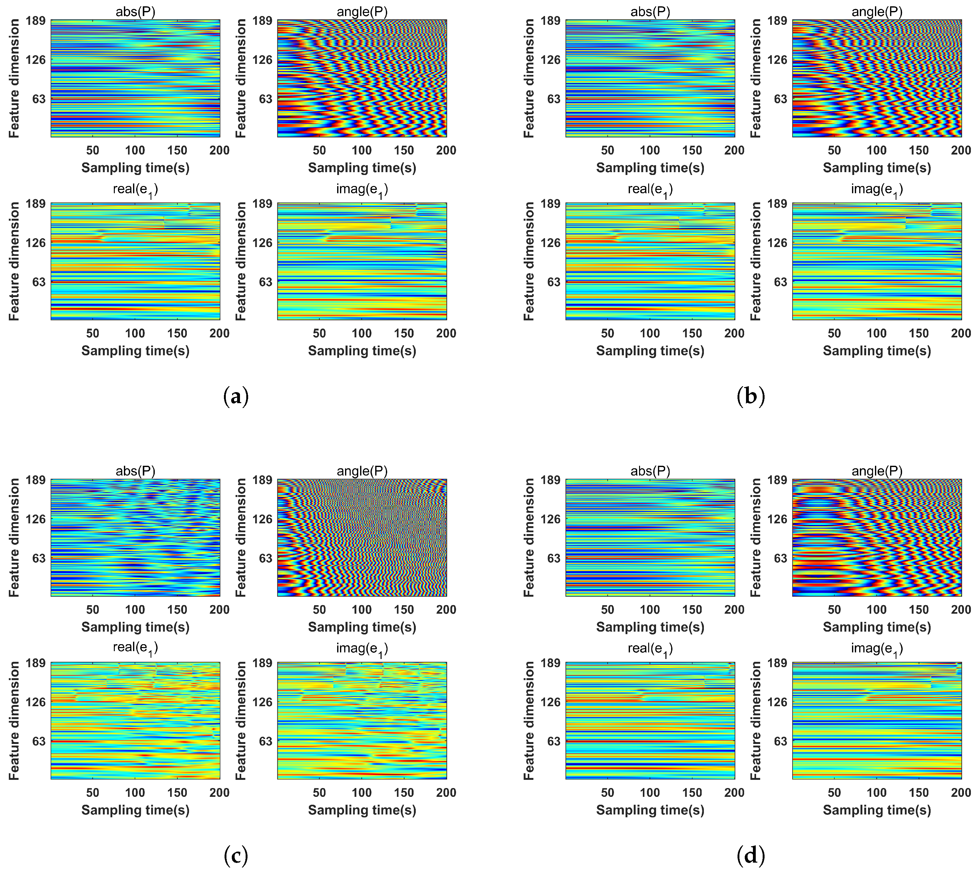
3.1. Different Input Features

In this section, we conduct two comparative experiments: the first comparing the localization performance of the proposed MTPEF features with other features and the second comparing the MTPEF features before and after augmentation. The localization performance is evaluated by RMSE.

In the first experiment, we contrasted the proposed MTPEF features with the following three features: the pressure and eigenvector feature (PEF), the multitime pressure feature (MTPF), and the multitime eigenvector feature (MTEF); the RMSE values trained on OriginNet are shown in

Table 2. The comparison of different input features.

Features	Element (at Each Frequency Point)	${\mathbf{RMSE}}_{\mathbf{depth}}$ (m)	${\mathbf{RMSE}}_{\mathbf{CPA}}$ (km)
PEF	${\left[\mathrm{abs}\left(\mathit{p}\left(f\right)\right)\mathrm{angle}\left(\mathit{p}\left(f\right)\right)\mathrm{real}\left({\mathit{e}}_{f1}\right)\mathrm{imag}\left({\mathit{e}}_{f1}\right)\right]}_{t=1}$	15.646	1.165
MTPF	${\left[\mathrm{abs}\left(\mathit{p}\left(f\right)\right)\mathrm{angle}\left(\mathit{p}\left(f\right)\right)\right]}_{t=N}$	9.385	1.001
MTEF	${\left[\mathrm{real}\left({\mathit{e}}_{f1}\right)\mathrm{imag}\left({\mathit{e}}_{f1}\right)\right]}_{t=N}$	8.733	1.094
MTPEF (ours)	${\left[\mathrm{abs}\left(\mathit{p}\left(f\right)\right)\mathrm{angle}\left(\mathit{p}\left(f\right)\right)\mathrm{real}\left({\mathit{e}}_{f1}\right)\mathrm{imag}\left({\mathit{e}}_{f1}\right)\right]}_{t=N}$	7.722	0.921

. The RMSE values of the four input features reached 15.65 m, 9.39 m, 8.73 m, and 7.72 m for the depth and reached 1.17 km, 1 km, 1.09 km, and 0.92 km for the CPA range. This indicates that the MTPEF obtained better localization performance than the case where a certain feature (MTPF or MTEF) was used alone and the case where only one sampling time (PEF) was used.

In the second experiment, we compared the localization results before and after feature augmentation. The test datasets were constructed such that the source velocity v ranges from 1 m/s to 10 m/s in steps of 1 m/s, and the time difference $\Delta t$ ranges from −200 s to 200 s in steps of 40 s. As shown in Figure 7, if the network model was trained by Train-A, only when the test datasets basically matched Train-A (v = 2.5 m/s and $\Delta t$ = 0 s), the RMSE values did not rise rapidly. Meanwhile, the network model trained by Train-B was not seriously affected when the target motion parameters changed. It can be concluded that the feature augmentation significantly improves the robustness of the network model.

3.2. Different Network Structures

In this section, we compare different network structures on the localization results. The MTPEF has been proven to achieve high accuracy on the baseline network structure OriginNet in Section 3.1, so it can be assumed that the localization accuracy of different networks is only affected by the structures rather than the input features. We contrast the proposed IRSNet with other neural network structures. Some are the structures that have been used in other fields, and others are the structures that replace the main module in Figure 4 with classical modules (such as ResNet18, ResNet34, and so on). The RMSE, the number of network parameters, and the training time of different network structures are shown in Table 3. The influence of various network structures can be summarized as follows:

• Compared the proposed IRSNet to the network structures that differ only in the main module, the localization accuracy of the IRSNet reached 3.657 m for the depth and 0.523 km for the CPA range. The network with only residual blocks and only inception modules was inferior to that of the IRSNet. The IRS module made the network localization accuracy further improved.
• The localization accuracies of the networks with residual modules and inception modules were generally better than that of the baseline network OriginNet. Deepening the network layers properly can not only improve the localization accuracy but also increase the training time. However, too many parameters can cause an increase in the RMSE, such as the results of the OriginNet with ResNet50 and the OriginNet with a 15 × V2 block. IRSNet has a reasonable number of parameters so that the network will not fall into overfitting. In addition, the lightweight transformation of the network reduces the training time without losing the localization accuracy.
• Compared the OriginNet with Inception-ResNet to the proposed IRSNet, although both structures use residual modules and inception modules together, the localization accuracy difference is huge. It shows that nesting inception modules and residual modules are too complicated and are not suitable structures for underwater acoustic localization. IRSNet connected the two kinds of modules in series and obtained a lower RMSE. In addition, the CNN-MTL [23] and CNN-Selkie3 [41] achieved good results in seabed parameter estimation, but the network structures could not directly transfer to the shallow water source localization because of the changes in input feature dimension and type. Improper network structures have a great influence on localization accuracy.

Table 3. Comparison of different network structures.

Network Structure	Parameter Number	Training Time (min)	${\mathbf{RMSE}}_{\mathbf{depth}}$ (m)	${\mathbf{RMSE}}_{\mathbf{CPA}}$ (km)
OriginNet (baseline)	$8.15\times {10}^5$	40	7.720	0.920
OriginNet with ResNet18	$1.11\times {10}^7$	73	4.647	0.755
OriginNet with ResNet34	$2.13\times {10}^7$	120	3.993	0.660
OriginNet with ResNet50	$2.35\times {10}^7$	177	12.930	1.758
OriginNet with 3 × V2 block	$4.51\times {10}^6$	77	4.074	0.634
OriginNet with 10 × V2 block	$1.02\times {10}^7$	153	3.721	0.668
OriginNet with 15 × V2 block	$2.17\times {10}^7$	187	5.178	0.972
OriginNet with Inception-ResNet	$2.10\times {10}^7$	227	21.097	2.433
CNN-Selkie3	$2.62\times {10}^7$	83	17.357	2.016
CNN-MTL	$3.21\times {10}^6$	23	14.335	1.287
IRSNet (ours)	$1.87\times {10}^7$	106	3.657	0.523

Table 3. Comparison of different network structures.

Network Structure	Parameter Number	Training Time (min)	${\mathbf{RMSE}}_{\mathbf{depth}}$ (m)	${\mathbf{RMSE}}_{\mathbf{CPA}}$ (km)
OriginNet (baseline)	$8.15\times {10}^5$	40	7.720	0.920
OriginNet with ResNet18	$1.11\times {10}^7$	73	4.647	0.755
OriginNet with ResNet34	$2.13\times {10}^7$	120	3.993	0.660
OriginNet with ResNet50	$2.35\times {10}^7$	177	12.930	1.758
OriginNet with 3 × V2 block	$4.51\times {10}^6$	77	4.074	0.634
OriginNet with 10 × V2 block	$1.02\times {10}^7$	153	3.721	0.668
OriginNet with 15 × V2 block	$2.17\times {10}^7$	187	5.178	0.972
OriginNet with Inception-ResNet	$2.10\times {10}^7$	227	21.097	2.433
CNN-Selkie3	$2.62\times {10}^7$	83	17.357	2.016
CNN-MTL	$3.21\times {10}^6$	23	14.335	1.287
IRSNet (ours)	$1.87\times {10}^7$	106	3.657	0.523

In conclusion, the IRSNet obtains high localization accuracy and short training time in all comparison networks, which has a suitable network structure and number of network parameters. The proposed IRSNet has been proven to be appropriate for acoustic source localization problems based on VLA.

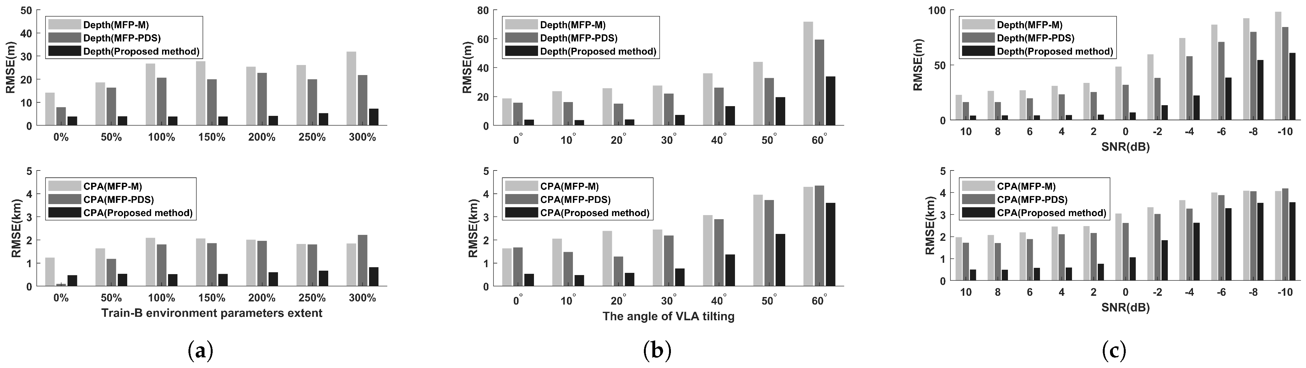
3.3. Comparison with Improved MFP Methods

In this section, we compare the proposed method with two improved MFP methods, named magnitude crossfrequency component MFP (MFP-M) in [9] and phase descent search method MFP (MFP-PDS) in [10]. We compare the methods under the environment mismatch conditions and give the visual localization results.

In order to compare the environment robustness of the methods, we created three types of environment mismatches. The first experiment changes the environment parameters perturbation size. The environment parameters of the test datasets vary from $0\%$ to $300\%$ of the Train-B environment parameters extent shown in Table 1. The second experiment changes the angle of the VLA, which varies from $0^{\circ }$ to ${60}^{\circ }$. The third experiment changes the SNR of the environment, which varies from −10 dB to 10 dB. The latter two experiments were conducted in 50% of the Train-B environment parameters extent.

As shown in Figure 8a, the proposed method had significantly stronger environment robustness than the MFP methods, and the RMSE remained low even for environment parameters that never appeared on the Train-B. When the angle of VLA and the SNR changed, the proposed method was less affected than the MFP methods. Assuming that ${\mathrm{RMSE}}_{\mathrm{depth}}\le$ 20 m and ${\mathrm{RMSE}}_{\mathrm{CPA}}\le$ 2 km are tolerable localization accuracies, according to Figure 8b and Figure 8c, the proposed method failed at ${60}^{\circ }$ VLA tilting and −4 dB SNR, while the MFP-PDS method failed at ${330}^{\circ }$ VLA tilting and 2 dB SNR.

We visualized a target with depth = 100 m and CPA range = 1 km using the MFP methods and the proposed method in Section 2.2.3, as shown in Figure 9. The MFP-PDS obviously suppressed the pseudopeak interference compared with the MFP-M, but it was still inevitably affected by the environment mismatch. The pseudopeak interference of the proposed method basically disappeared, and the closer the area was to the actual source location, the higher the correlation degree. This can prove that the network has learned the probability distribution. In addition, when we set the threshold at $\zeta =0.95$, the LCI gave a high-confidence depth range and a CPA range of 87–116 m and 0.7–1.4 km.

In conclusion, the proposed method has higher environment robustness than the MFP methods, and the visualization results back this conclusion up.

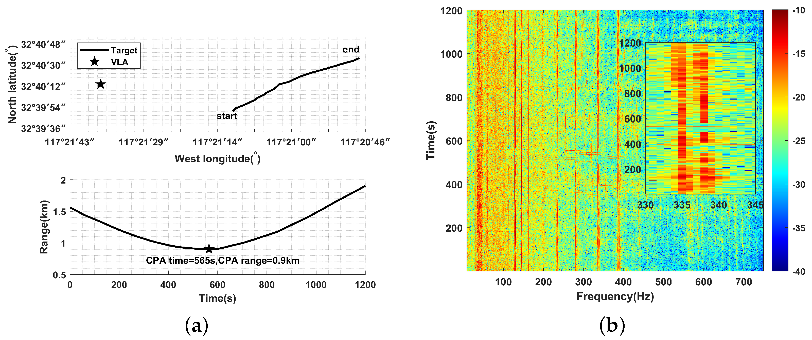
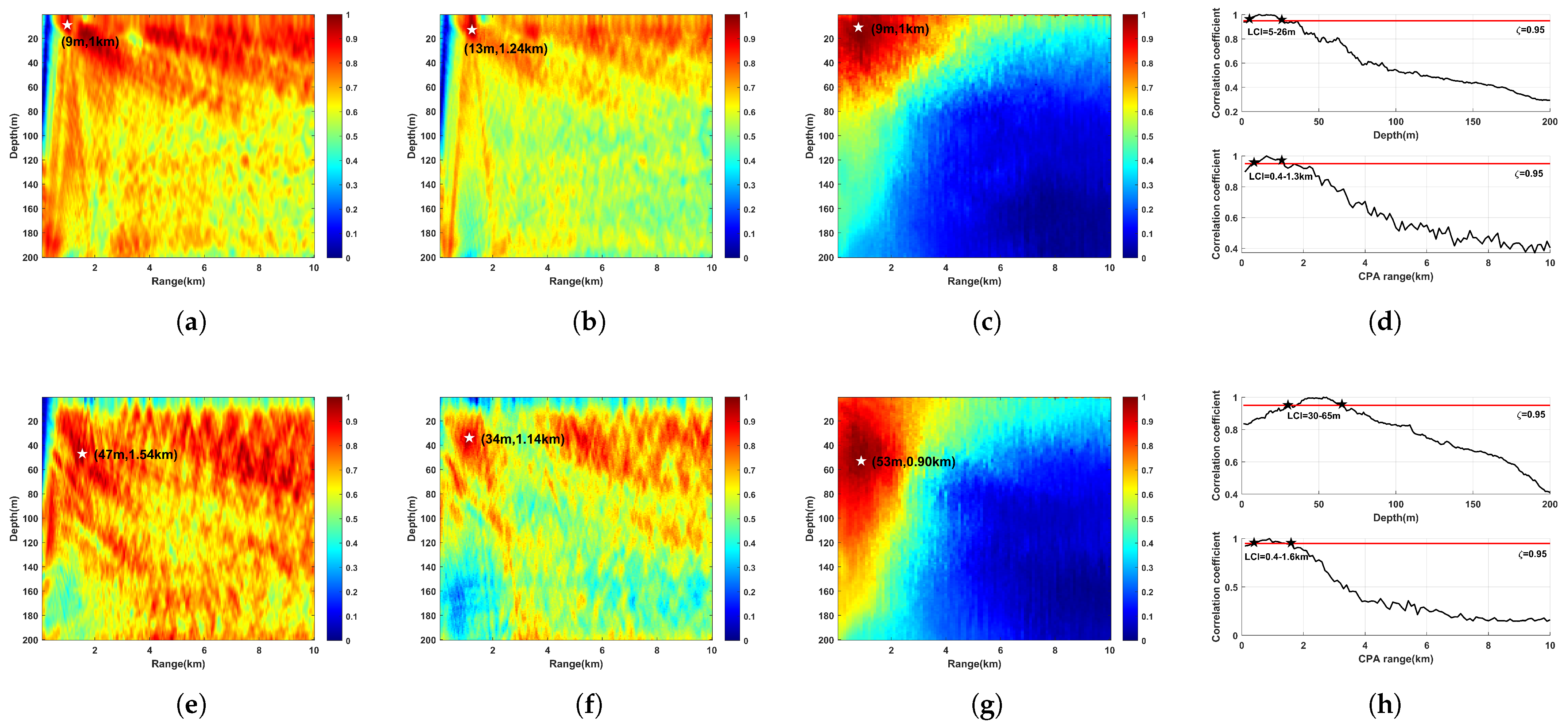
3.4. Evaluation on SWellEx-96 Experiment

SWellEx-96 is an experiment conducted by the University of California San Diego Marine Physical Lab in the waters off Point Loma between 10–18 May 1996. During the partial motion in the S5 event, the source ship traveled north from the south side of the emplaced VLA at about 2.5 m/s from 00:05 on May 11, and a GPS recorded the track of 1200 s. A deep source of about 54 m and a shallow source of about 9 m are towed simultaneously, and both sources emitted varied single-frequency signals with frequencies between 49 and 400 Hz. As shown in Figure 10a, the GPS was read to obtain the distance variation between the source ship and the VLA, and the source ship reached the CPA point at 565 s, when the CPA range = 0.902 km. As shown in Figure 10b, the doppler shift phenomenon of a specific frequency on the acoustic source also proves the credibility of the CPA moment, which is estimated at about 570 s on the LOFAR.

The localization results obtained by MFP-M, MFP-PDS, and the proposed method are shown in Table 4. The proposed method was less affected by environmental mismatches; in particular, the localization result of the deep source was closer to the actual situation than the MFP methods. The trained network only needed to make parameter calls, and the computation speed was about four times faster than the MFP methods. The visualization results are shown in Figure 11. The proposed method had less sidelobe interference compared to the MFP methods. The LCI gave a high confidence depth range, and the CPA range was 5–26 m and 0.4–1.3 km for the shallow source, while it was 30–65 m and 0.4–1.6 km for the deep source.

Table 4. Comparison of different network structures.

Method	Shallow Source		Deep Source		Running Time
	Depth (Error)	CPA Range (Error)	Depth (Error)	CPA Range (Error)
MFP-M	9 m (0 m)	1 km (+0.1 km)	47 m (−7 m)	1.54 km (+0.64 km)	7.2 s
MFP-PDS	13 m (+4 m)	1.24 km (+0.34 km)	34 m (−20 m)	1.14 km (+0.24 km)	8.9 s
Proposed method	9 m (0 m)	1 km (0.1 km)	53 m (−1 m)	0.90 km (0 km)	2 s

Table 4. Comparison of different network structures.

Method	Shallow Source		Deep Source		Running Time
	Depth (Error)	CPA Range (Error)	Depth (Error)	CPA Range (Error)
MFP-M	9 m (0 m)	1 km (+0.1 km)	47 m (−7 m)	1.54 km (+0.64 km)	7.2 s
MFP-PDS	13 m (+4 m)	1.24 km (+0.34 km)	34 m (−20 m)	1.14 km (+0.24 km)	8.9 s
Proposed method	9 m (0 m)	1 km (0.1 km)	53 m (−1 m)	0.90 km (0 km)	2 s

Figure 11. The visualization results of the shallow source and the deep source: (a) MFP-M on shallow source. (b) MFP-PDS on shallow source. (c) Proposed method on shallow source. (d) The LCI on shallow source. (e) MFP-M on deep source. (f) MFP-PDS on deep source. (g) Proposed method on deep source. (h) The LCI on deep source.

Figure 11. The visualization results of the shallow source and the deep source: (a) MFP-M on shallow source. (b) MFP-PDS on shallow source. (c) Proposed method on shallow source. (d) The LCI on shallow source. (e) MFP-M on deep source. (f) MFP-PDS on deep source. (g) Proposed method on deep source. (h) The LCI on deep source.

4. Discussion

Due to the mismatch in complex ocean environments, the past MFP methods are difficult to apply. Many neural network methods directly transfer the classical features and network structures to underwater acoustic localization problems and still have room for improvement in accuracy. Aiming at solving the shortcomings of those methods, the proposed method mainly involves the following three parts. Firstly, we put forward a feature preprocessing scheme. The MTPEF features in the feature processing step are proposed to improve the localization accuracy. Meanwhile, feature augmentation is used to improve the localization robustness. Secondly, we design a deep network structure IRSNet. The IRSNet takes into account the advantages of the multiscale convolution kernel and the residual structure, which can enhance the localization accuracy. Finally, we propose a network visualization method to prove the ability of the proposed method, and the LCI is defined to optimize the estimated localization results.

Subsequent research will be categorized into three main directions. Firstly, our research focuses on the shallow water passive source localization problem. It should be noted that the environment can be divided into shallow water and deep water based on varying water depths, and the modeling methods are different. Whether the proposed method is applicable to deep water localization problem is a future research direction. Secondly, the design of network parameter quantity is based on the empirical value obtained from simulation results. If the type and dimension of input features are changed, the impact on the network parameter quantity needs to be further studied. Finally, our research can be extended from single target localization to multitarget localization.

5. Conclusions

In this article, a deep learning localization method via improved input features and network structure has been proposed to estimate the depth and the CPA range for shallow water passive source. The simulation results have proven that the improved input feature MTPEF has the best localization accuracy compared to the other three features, and it is robust to both environment parameters and target motion parameters. Taking into account training time and localization accuracy, the proposed IRSNet structure is superior compared to the other ten network structures. Additionally, the proposed method has higher environment robustness than the improved MFP methods in three types of mismatch, which is further supported by the visualization method. The SWellEX-96 experimental results validate the localization efficiency and accuracy of the proposed method.

References

1. Zhang, T.; Han, G.; Guizani, M.; Yan, L.; Shu, L. Peak Extraction Passive Source Localization Using a Single Hydrophone in Shallow Water. IEEE Trans. Veh. Technol. 2020, 69, 3412–3423. [Google Scholar] [CrossRef]
2. Weiss, A.; Arikan, T.; Vishnu, H.; Deane, G.B.; Singer, A.C.; Wornell, G.W. A Semi-Blind Method for Localization of Underwater Acoustic Sources. IEEE Trans. Signal Process. 2022, 70, 3090–3106. [Google Scholar] [CrossRef]
3. Le Gall, Y.; Socheleau, F.X.; Bonnel, J. Matched-Field Processing Performance Under the Stochastic and Deterministic Signal Models. IEEE Trans. Signal Process. 2014, 62, 5825–5838. [Google Scholar] [CrossRef]
4. Finette, S.; Mignerey, P.C. Stochastic matched-field localization of an acoustic source based on principles of Riemannian geometry. J. Acoust. Soc. Am. 2018, 143, 3628–3638. [Google Scholar] [CrossRef] [PubMed]
5. Westwood, E.K. Broadband matched-field source localization. J. Acoust. Soc. Am. 1992, 91, 2777–2789. [Google Scholar] [CrossRef]
6. Zhang, R.; Li, Z.; Yan, J.; Peng, Z.; Li, F. Broad-band matched-field source localization in the east China Sea. IEEE J. Ocean. Eng. 2004, 29, 1049–1054. [Google Scholar] [CrossRef]
7. Michalopoulou, Z.H.; Pole, A.; Abdi, A. Bayesian coherent and incoherent matched-field localization and detection in the ocean. J. Acoust. Soc. Am. 2019, 146, 4812–4820. [Google Scholar] [CrossRef] [PubMed]
8. Virovlyansky, A.L.; Kazarova, A.Y.; Lyubavin, L.Y. Matched Field Processing in Phase Space. IEEE J. Ocean. Eng. 2020, 45, 1583–1593. [Google Scholar] [CrossRef]
9. Orris, G.J.; Nicholas, M.; Perkins, J.S. The matched-phase coherent multi-frequency matched-field processor. J. Acoust. Soc. Am. 2000, 107, 2563–2575. [Google Scholar] [CrossRef]
10. Chen, T.; Liu, C.; Zakharov, Y.V. Source Localization Using Matched-Phase Matched-Field Processing With Phase Descent Search. IEEE J. Ocean. Eng. 2012, 37, 261–270. [Google Scholar] [CrossRef]
11. Yang, T. Data-based matched-mode source localization for a moving source. J. Acoust. Soc. Am. 2014, 135, 1218–1230. [Google Scholar] [CrossRef] [PubMed]
12. Virovlyansky, A. Stable components of sound fields in the ocean. J. Acoust. Soc. Am. 2017, 141, 1180–1189. [Google Scholar] [CrossRef] [PubMed]
13. Aravindan, S.; Ramachandran, N.; Naidu, P.S. Fast matched field processing. IEEE J. Ocean. Eng. 1993, 18, 1–5. [Google Scholar] [CrossRef]
14. Sun, Z.; Meng, C.; Cheng, J.; Zhang, Z.; Chang, S. A multi-scale feature pyramid network for detection and instance segmentation of marine ships in SAR images. Remote Sens. 2022, 14, 6312. [Google Scholar] [CrossRef]
15. Zhu, X.C.; Zhang, H.; Feng, H.T.; Zhao, D.H.; Zhang, X.J.; Tao, Z. IFAN: An Icosahedral Feature Attention Network for Sound Source Localization. IEEE Trans. Instrum. Meas. 2024, 73, 1–13. [Google Scholar] [CrossRef]
16. Li, Y.; Si, Y.; Tong, Z.; He, L.; Zhang, J.; Luo, S.; Gong, Y. MQANet: Multi-Task Quadruple Attention Network of Multi-Object Semantic Segmentation from Remote Sensing Images. Remote Sens. 2022, 14, 6256. [Google Scholar] [CrossRef]
17. Bianco, M.J.; Gerstoft, P.; Traer, J.; Ozanich, E.; Roch, M.A.; Gannot, S.; Deledalle, C.A. Machine learning in acoustics: Theory and applications. J. Acoust. Soc. Am. 2019, 146, 3590–3628. [Google Scholar] [CrossRef] [PubMed]
18. Michalopoulou, Z.H.; Gerstoft, P.; Kostek, B.; Roch, M.A. Introduction to the special issue on machine learning in acoustics. J. Acoust. Soc. Am. 2021, 150, 3204–3210. [Google Scholar] [CrossRef] [PubMed]
19. Zhou, T.; Wang, Y.; Zhang, L.; Chen, B.; Yu, X. Underwater Multitarget Tracking Method Based on Threshold Segmentation. IEEE J. Ocean. Eng. 2023, 48, 1255–1269. [Google Scholar] [CrossRef]
20. Wang, Y.; Peng, H. Underwater acoustic source localization using generalized regression neural network. J. Acoust. Soc. Am. 2018, 143, 2321–2331. [Google Scholar] [CrossRef]
21. Niu, H.; Reeves, E.; Gerstoft, P. Source localization in an ocean waveguide using supervised machine learning. J. Acoust. Soc. Am. 2017, 142, 1176–1188. [Google Scholar] [CrossRef] [PubMed]
22. Zhu, X.; Dong, H.; Salvo Rossi, P.; Landrø, M. Feature selection based on principal component regression for underwater source localization by deep learning. Remote Sens. 2021, 13, 1486. [Google Scholar] [CrossRef]
23. Neilsen, T.; Escobar-Amado, C.; Acree, M.; Hodgkiss, W.; Van Komen, D.; Knobles, D.; Badiey, M.; Castro-Correa, J. Learning location and seabed type from a moving mid-frequency source. J. Acoust. Soc. Am. 2021, 149, 692–705. [Google Scholar] [CrossRef] [PubMed]
24. Shin, H.C.; Roth, H.R.; Gao, M.; Lu, L.; Xu, Z.; Nogues, I.; Yao, J.; Mollura, D.; Summers, R.M. Deep convolutional neural networks for computer-aided detection: CNN architectures, dataset characteristics and transfer learning. IEEE Trans. Med. Imaging 2016, 35, 1285–1298. [Google Scholar] [CrossRef] [PubMed]
25. Sun, D.; Jia, Z.; Teng, T.; Ma, C. Robust high-resolution direction-of-arrival estimation method using DenseBlock-based U-net. J. Acoust. Soc. Am. 2022, 151, 3426–3436. [Google Scholar] [CrossRef] [PubMed]
26. Sun, S.; Liu, T.; Wang, Y.; Zhang, G.; Liu, K.; Wang, Y. High-rate underwater acoustic localization based on the decision tree. IEEE Trans. Geosci. Remote Sens. 2021, 60, 4204912. [Google Scholar] [CrossRef]
27. Niu, H.; Gong, Z.; Ozanich, E.; Gerstoft, P.; Wang, H.; Li, Z. Deep-learning source localization using multi-frequency magnitude-only data. J. Acoust. Soc. Am. 2019, 146, 211–222. [Google Scholar] [CrossRef] [PubMed]
28. Huang, Z.; Xu, J.; Gong, Z.; Wang, H.; Yan, Y. Source localization using deep neural networks in a shallow water environment. J. Acoust. Soc. Am. 2018, 143, 2922–2932. [Google Scholar] [CrossRef]
29. Qian, P.; Gan, W.; Niu, H.; Ji, G.; Li, Z.; Li, G. A feature-compressed multi-task learning U-Net for shallow-water source localization in the presence of internal waves. Appl. Acoust. 2023, 211, 109530. [Google Scholar] [CrossRef]
30. Wang, W.; Ni, H.; Su, L.; Hu, T.; Ren, Q.; Gerstoft, P.; Ma, L. Deep transfer learning for source ranging: Deep-sea experiment results. J. Acoust. Soc. Am. 2019, 146, EL317–EL322. [Google Scholar] [CrossRef]
31. Agrawal, S.; Sharma, D.K. Feature extraction and selection techniques for time series data classification: A comparative analysis. In Proceedings of the 2022 9th International Conference on Computing for Sustainable Global Development (INDIACom), New Delhi, India, 23–25 March 2022; pp. 860–865. [Google Scholar]
32. Richardson, A.; Nolte, L. A posteriori probability source localization in an uncertain sound speed, deep ocean environment. J. Acoust. Soc. Am. 1991, 89, 2280–2284. [Google Scholar] [CrossRef]
33. Schaeffer-Filho, A.; Smith, P.; Mauthe, A.; Hutchison, D.; Yu, Y.; Fry, M. A framework for the design and evaluation of network resilience management. In Proceedings of the 2012 IEEE Network Operations and Management Symposium, Maui, HI, USA, 16–20 April 2012; pp. 401–408. [Google Scholar]
34. Szegedy, C.; Liu, W.; Jia, Y.; Sermanet, P.; Reed, S.; Anguelov, D.; Erhan, D.; Vanhoucke, V.; Rabinovich, A. Going deeper with convolutions. In Proceedings of the IEEE Conference on Computer Vision and Pattern Recognition, Boston, MA, USA, 7–12 June 2015; pp. 1–9. [Google Scholar]
35. Lu, N.; Li, T.; Ren, X.; Miao, H. A deep learning scheme for motor imagery classification based on restricted Boltzmann machines. IEEE Trans. Neural Syst. Rehabil. Eng. 2016, 25, 566–576. [Google Scholar] [CrossRef] [PubMed]
36. Saha, A.; Rathore, S.S.; Sharma, S.; Samanta, D. Analyzing the difference between deep learning and machine learning features of EEG signal using clustering techniques. In Proceedings of the 2019 IEEE Region 10 Symposium (TENSYMP), Kolkata, India, 7–9 June 2019; pp. 660–664. [Google Scholar]
37. He, K.; Zhang, X.; Ren, S.; Sun, J. Deep residual learning for image recognition. In Proceedings of the IEEE Conference on Computer Vision and Pattern Recognition, Las Vegas, NV, USA, 27–30 June 2016; pp. 770–778. [Google Scholar]
38. Szegedy, C.; Vanhoucke, V.; Ioffe, S.; Shlens, J.; Wojna, Z. Rethinking the inception architecture for computer vision. In Proceedings of the IEEE Conference on Computer Vision and Pattern Recognition, Las Vegas, NV, USA, 27–30 June 2016; pp. 2818–2826. [Google Scholar]
39. Szegedy, C.; Ioffe, S.; Vanhoucke, V.; Alemi, A. Inception-v4, inception-resnet and the impact of residual connections on learning. In Proceedings of the AAAI Conference on Artificial Intelligence, San Francisco, CA, USA, 4–9 February 2017; Volume 31. [Google Scholar]
40. Zeiler, M.D.; Fergus, R. Visualizing and understanding convolutional networks. In Proceedings of the Computer Vision–ECCV 2014: 13th European Conference, Zurich, Switzerland, 6–12 September 2014; pp. 818–833. [Google Scholar]
41. Van Komen, D.F.; Neilsen, T.B.; Mortenson, D.B.; Acree, M.C.; Knobles, D.P.; Badiey, M.; Hodgkiss, W.S. Seabed type and source parameters predictions using ship spectrograms in convolutional neural networks. J. Acoust. Soc. Am. 2021, 149, 1198–1210. [Google Scholar] [CrossRef] [PubMed]
Figure 1. The overall feature processing step of the MTPEF.
Remotesensing 16 01391 g001
Figure 4. The overall deep network structure of the IRSNet.
Remotesensing 16 01391 g004
Figure 5. The overall calculation processing flow of the LCI.
Remotesensing 16 01391 g005
Figure 6. The simulation shallow waveguide environment.
Remotesensing 16 01391 g006
Figure 7. The RMSE values of the network trained by Train-A and Train-B: (a) The source velocity v varied from 1 m/s to 10 m/s. (b) The time difference Δ t varied from −200 s to 200 s.
Remotesensing 16 01391 g007
Figure 8. The RMSE of MFP-M, MFP-PDS, and proposed method in different environment mismatch cases: (a) The different environment mismatch extent according to Train-B. (b) The different angle of VLA tilting. (c) The different SNR condition.
Remotesensing 16 01391 g008
Figure 9. The visualization results of the simulation target: (a) MFP-M. (b) MFP-PDS. (c) Proposed method. (d) The LCI. The true value of the simulation target is depth = 100 m and CPA range = 1 km.
Remotesensing 16 01391 g009aRemotesensing 16 01391 g009b
Figure 10. The GPS and LOFAR results of SWellEx-96: (a) GPS between 00:05 and 0:25 on May 11. (b) LOFAR between 00:05 and 0:25 on 11 May.
Remotesensing 16 01391 g010