

Estimation of All-Day Aerosol Optical Depth in the Beijing–Tianjin–Hebei Region Using Ground Air Quality Data


Abstract
1. Introduction
2. Materials and Methods
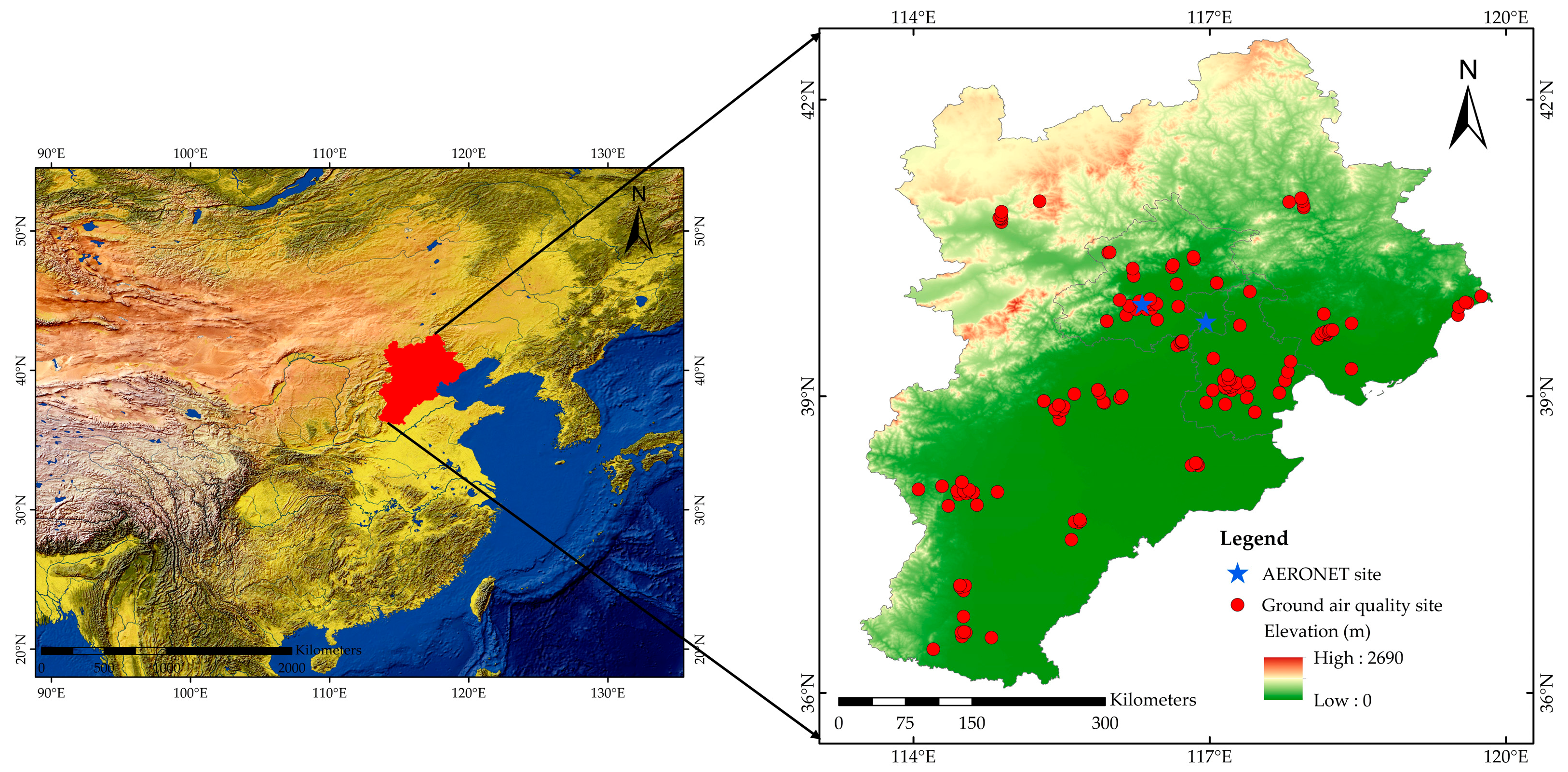
2.1. Datasets
2.1.1. Ground Air Quality Data
2.1.2. Meteorological Data
2.1.3. AHI AOD
2.1.4. AERONET AOD
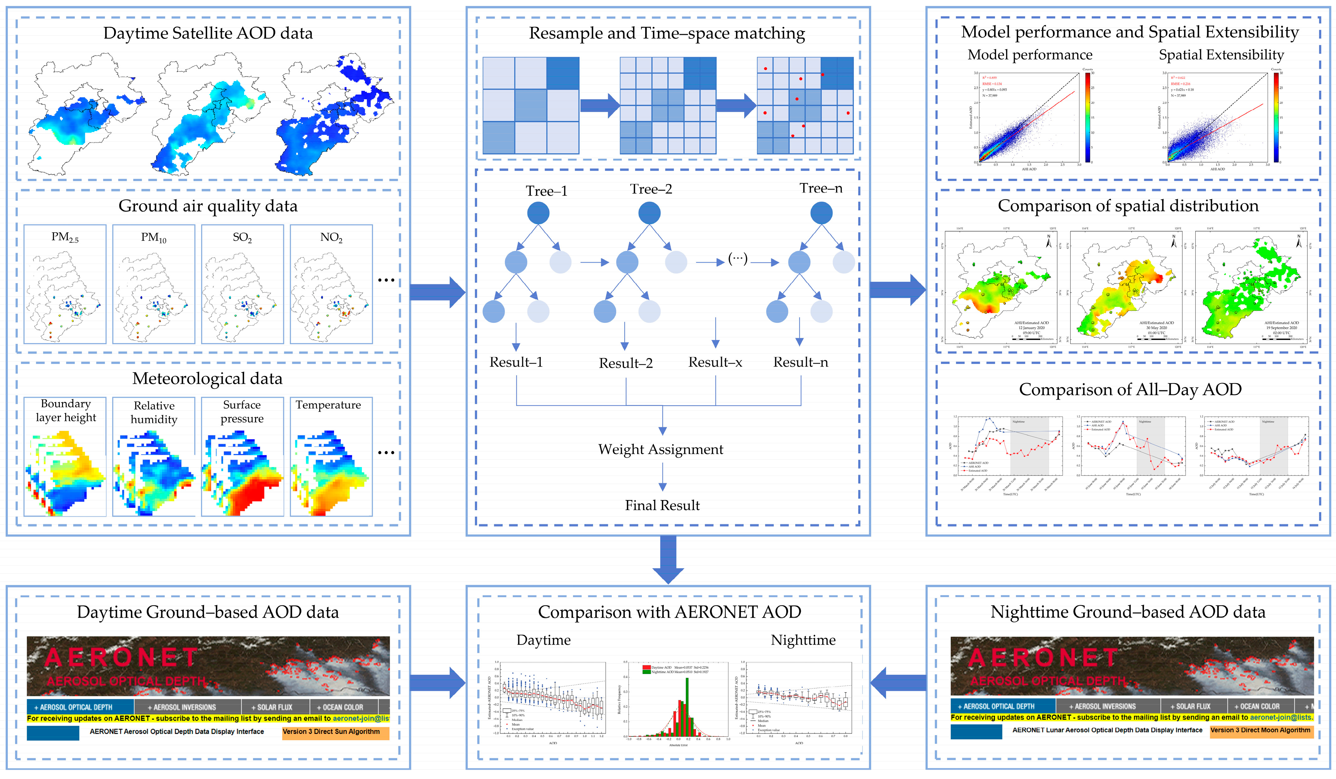
2.2. Methods
2.2.1. Data Preprocessing
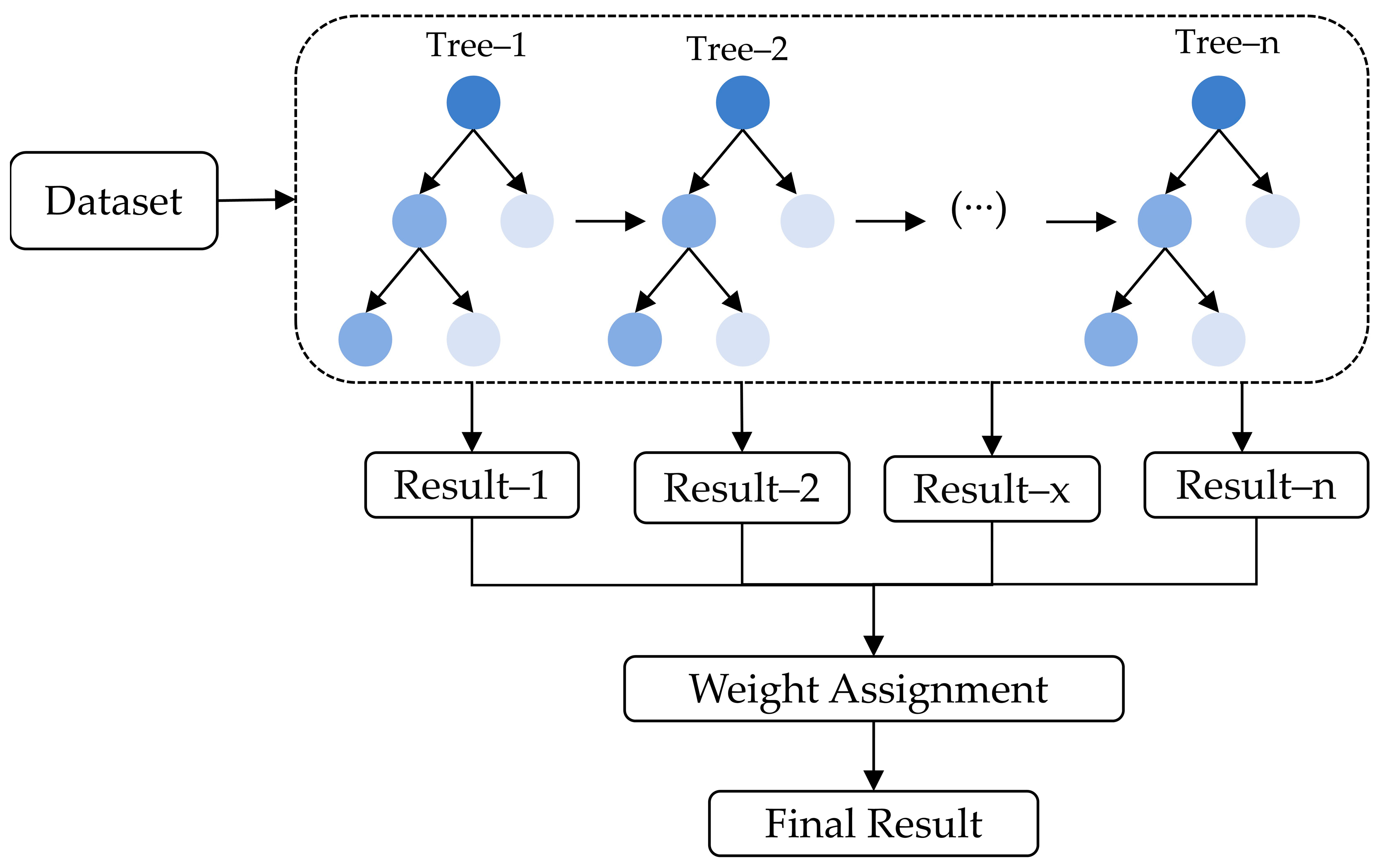
2.2.2. All-Day AODES
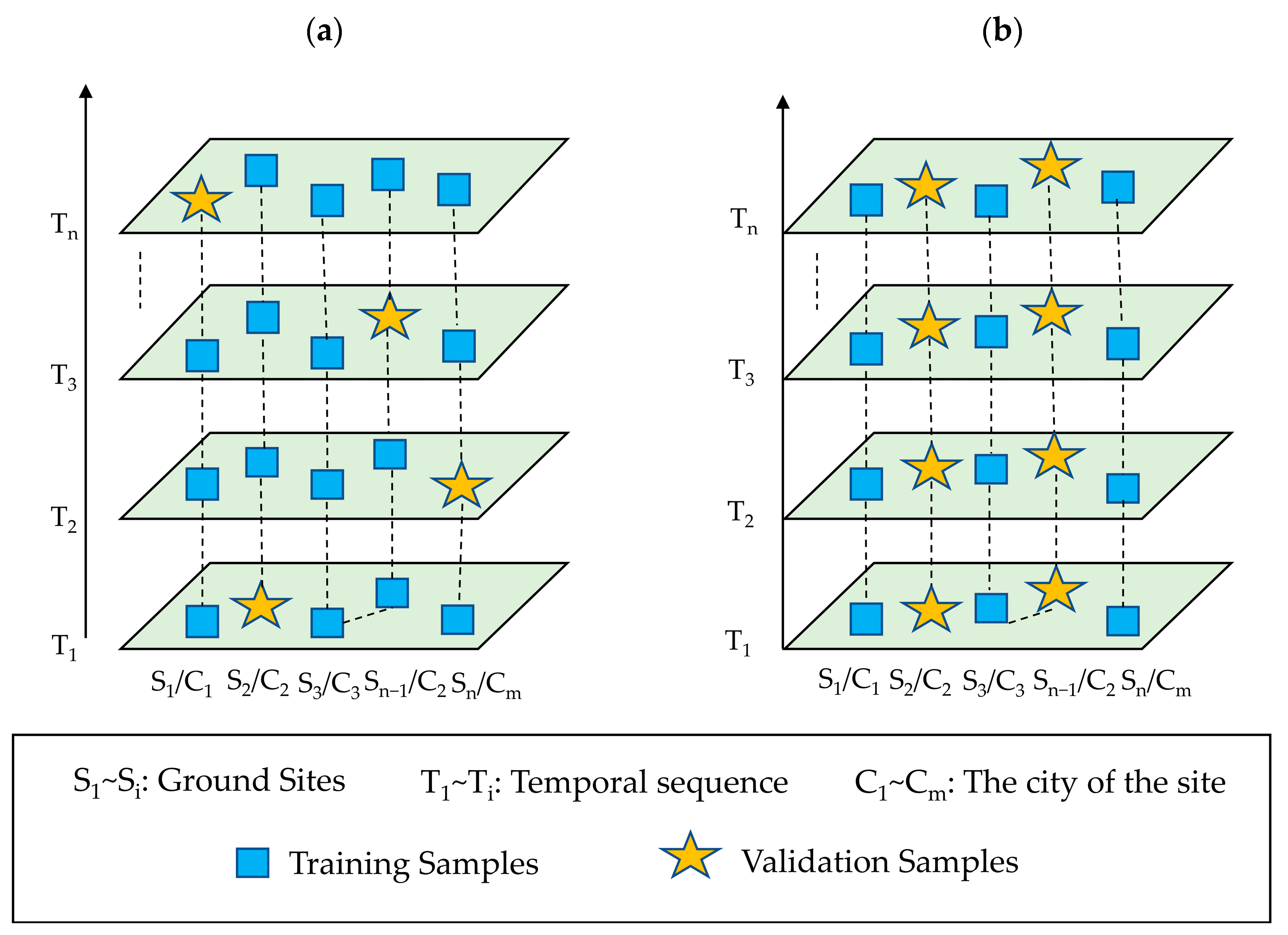
2.2.3. System Model Evaluation
- 1.
- Sample–based cross–validation involves partitioning the dataset into ten subsets and performing ten cycles. In each process, nine subsets were used as training data, whereas the remaining subsets served as validation data. The performance of the final trained model was evaluated using a test dataset.
- 2.
- Leave–one–city cross–validation involves partitioning the dataset according to the “city” attribute. This study encompasses a total of 13 cities. In each iteration, data from one city served as the validation set, whereas data from the remaining 12 cities constituted the training set. During each iteration, the model was trained on the training set and subsequently evaluated on the test dataset.
3. Results
3.1. Estimation of All-Day AOD
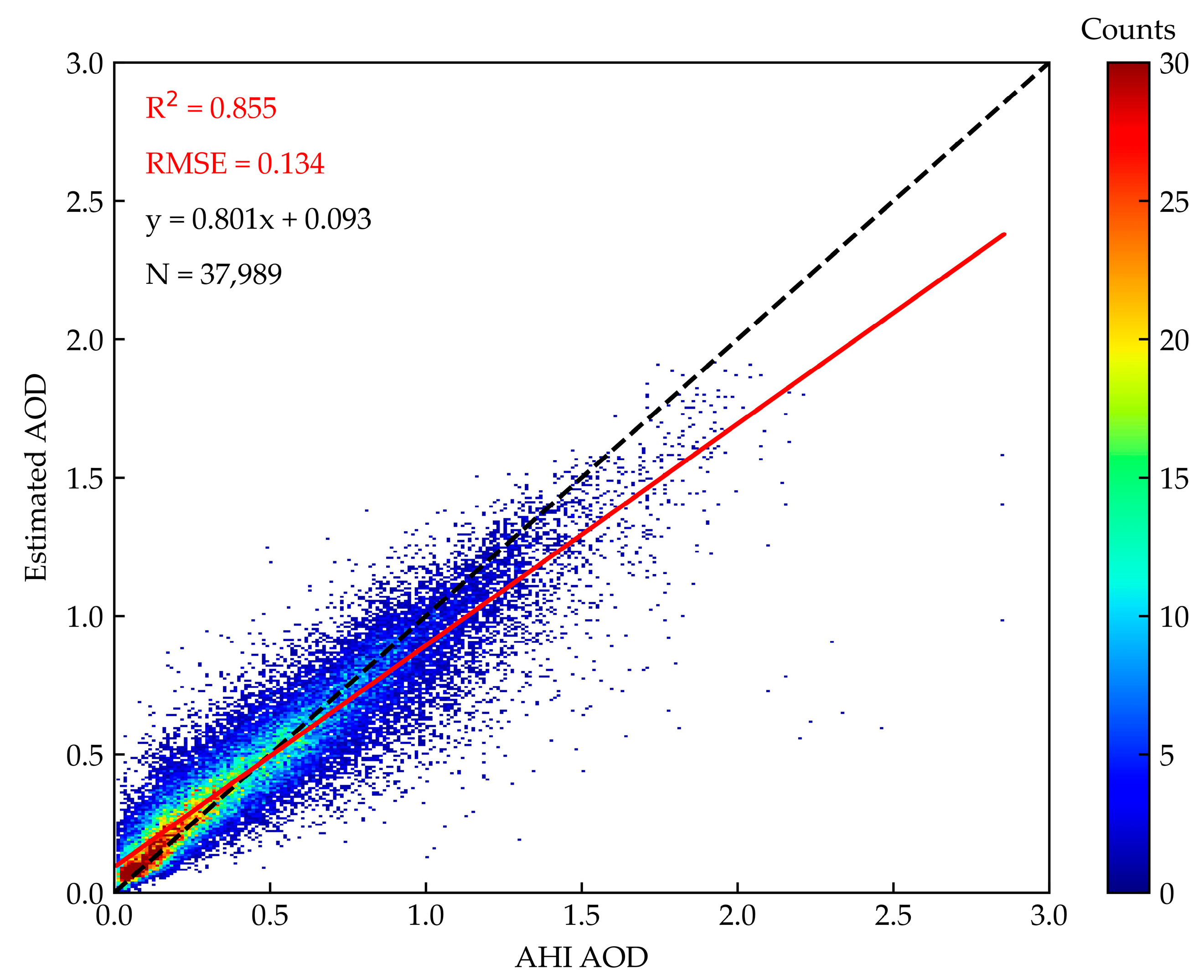
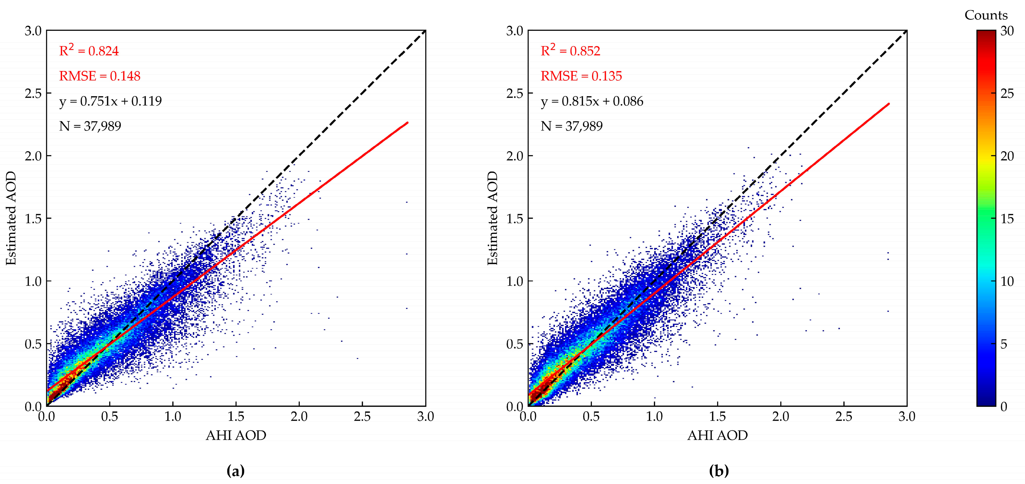
3.1.1. Analytical Comparison of Different Models
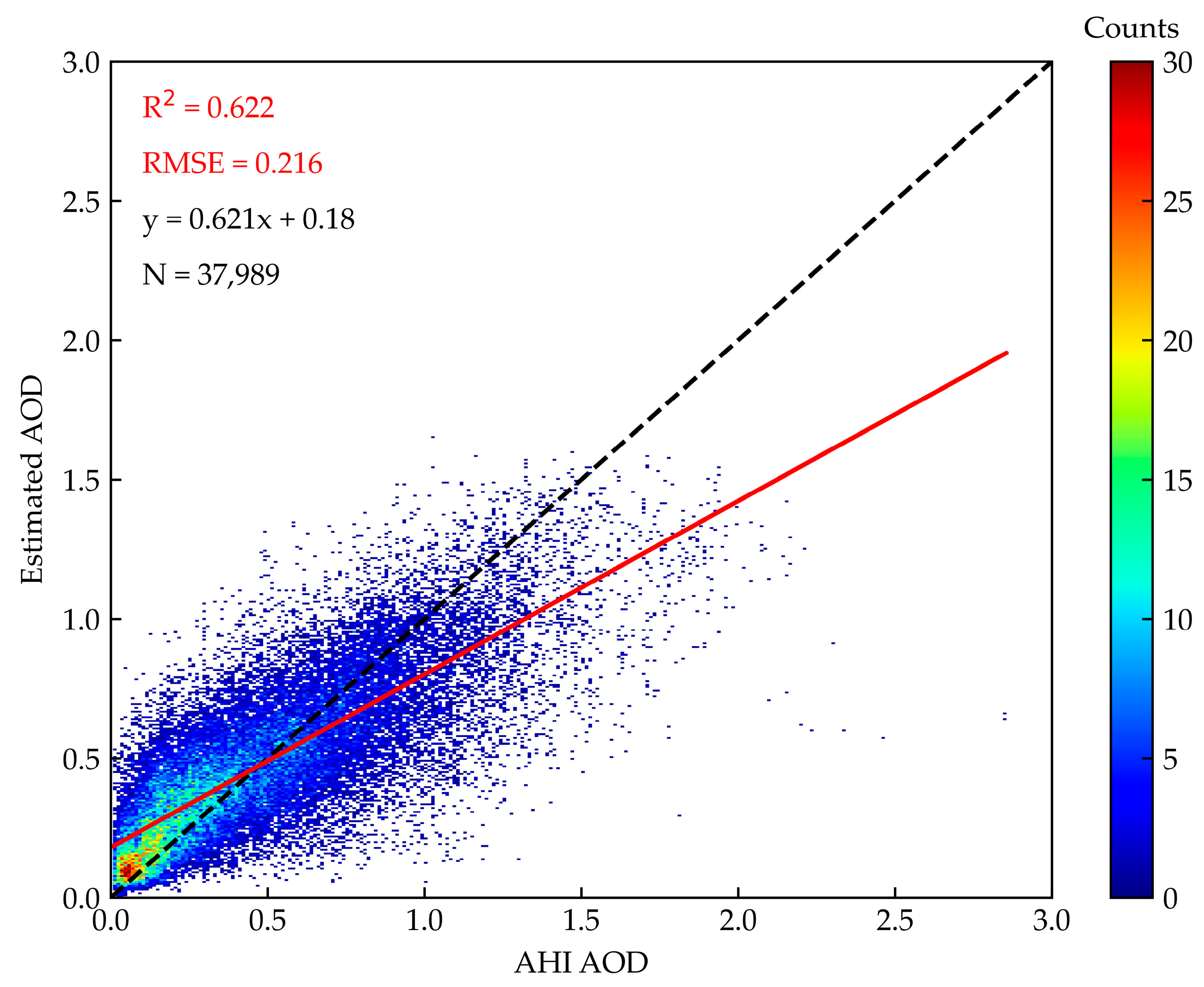
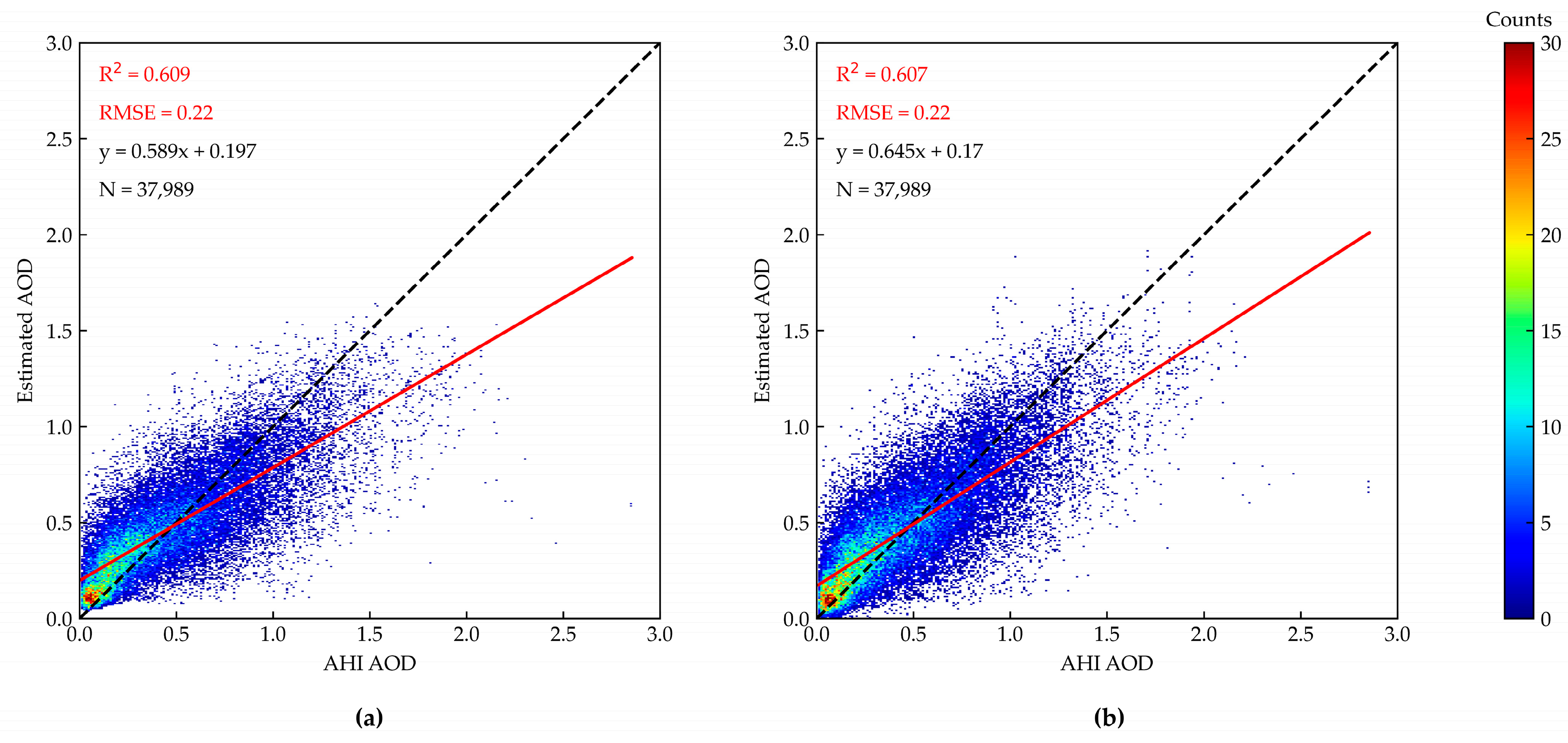
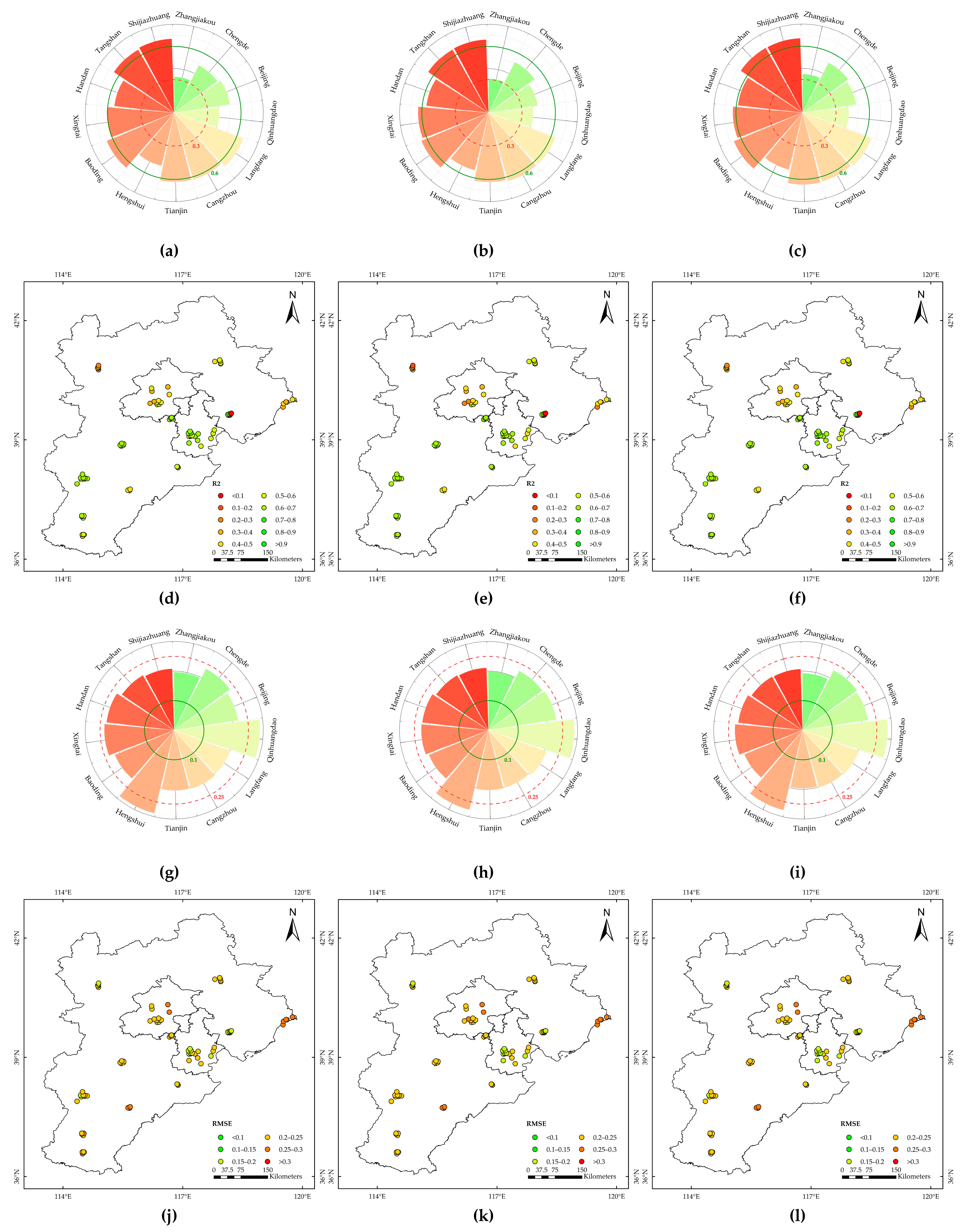
3.1.2. Spatial Extensibility of Different Models
3.2. Verification of All-Day AOD
3.2.1. Comparison with AERONET AOD
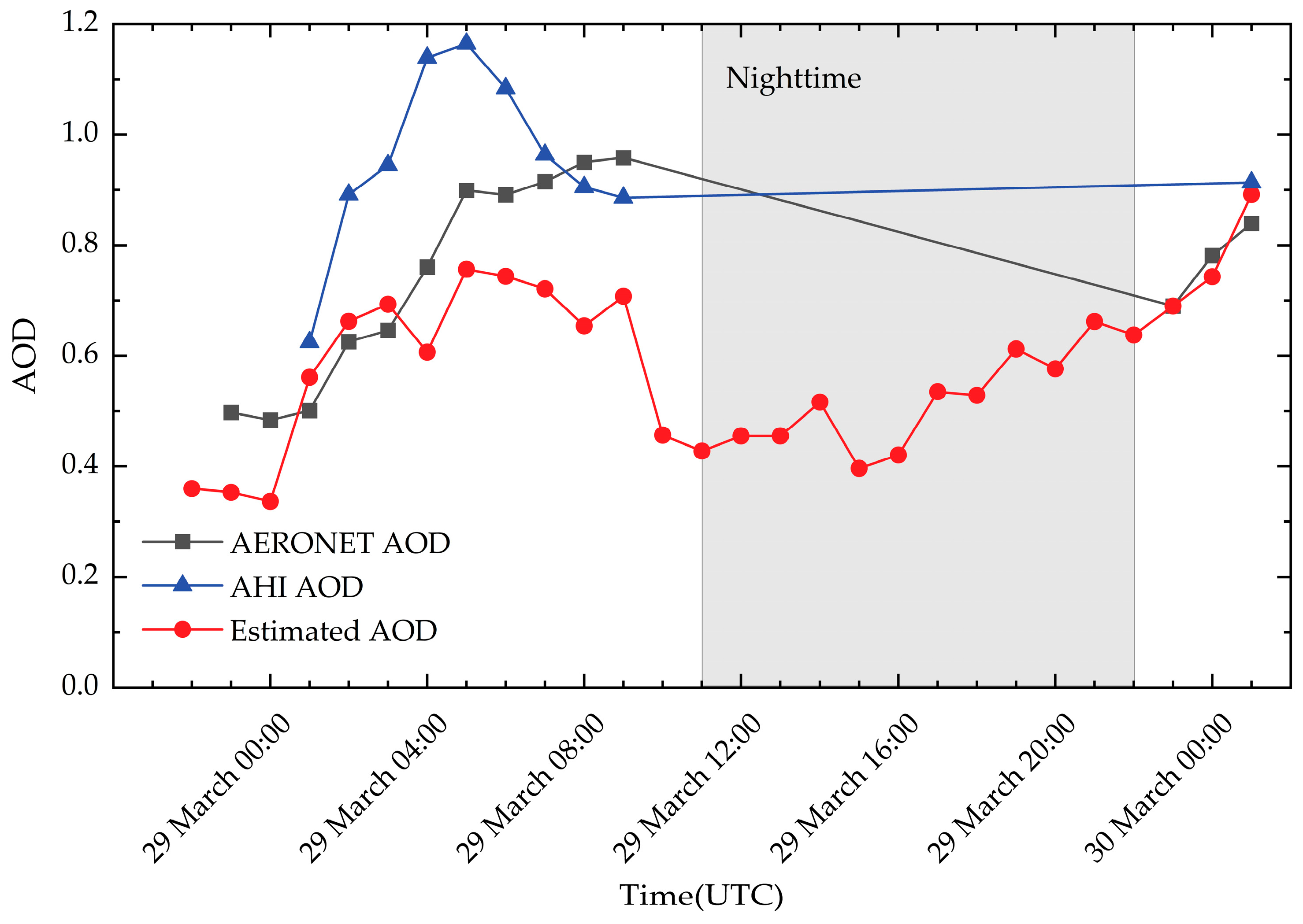
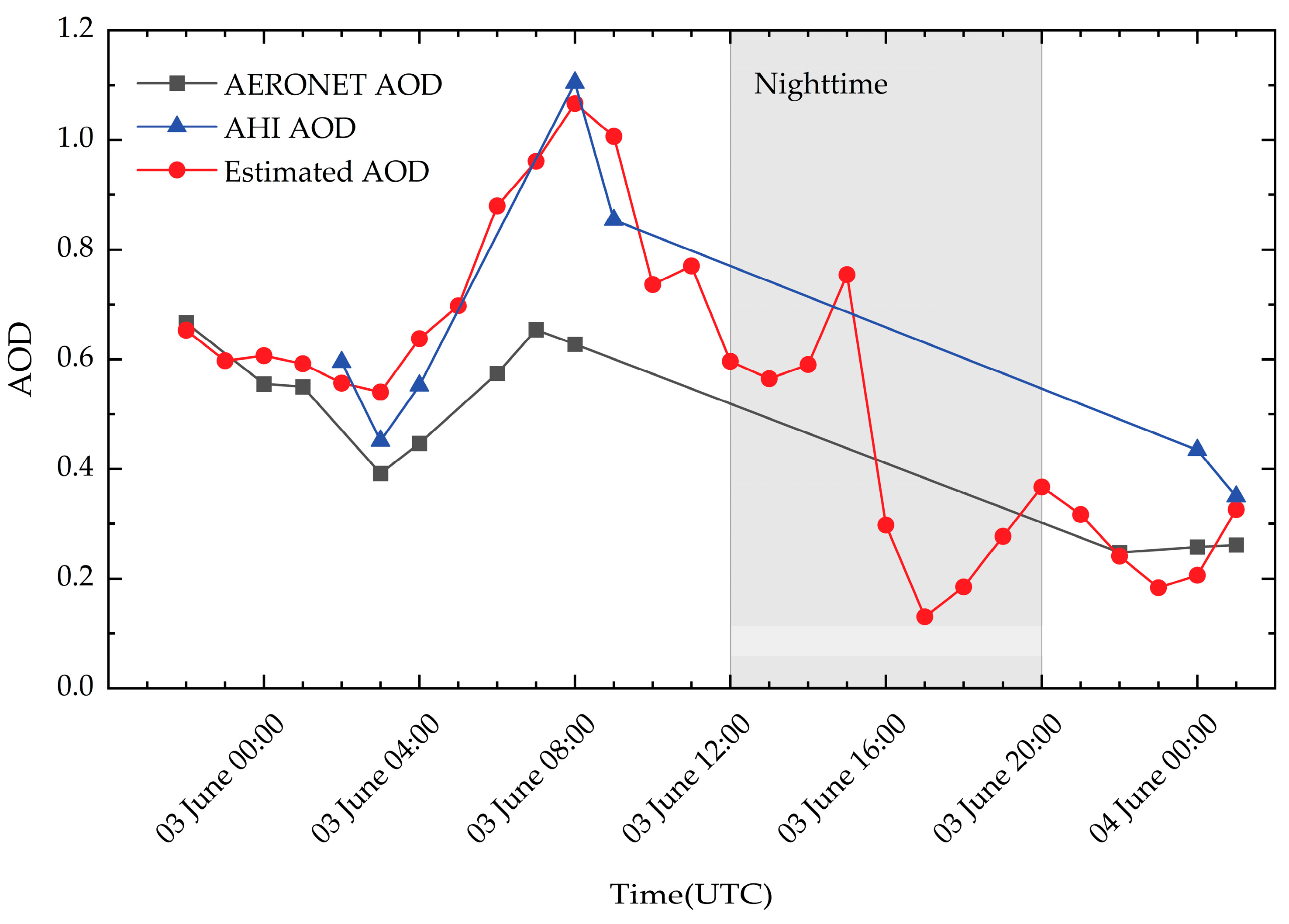
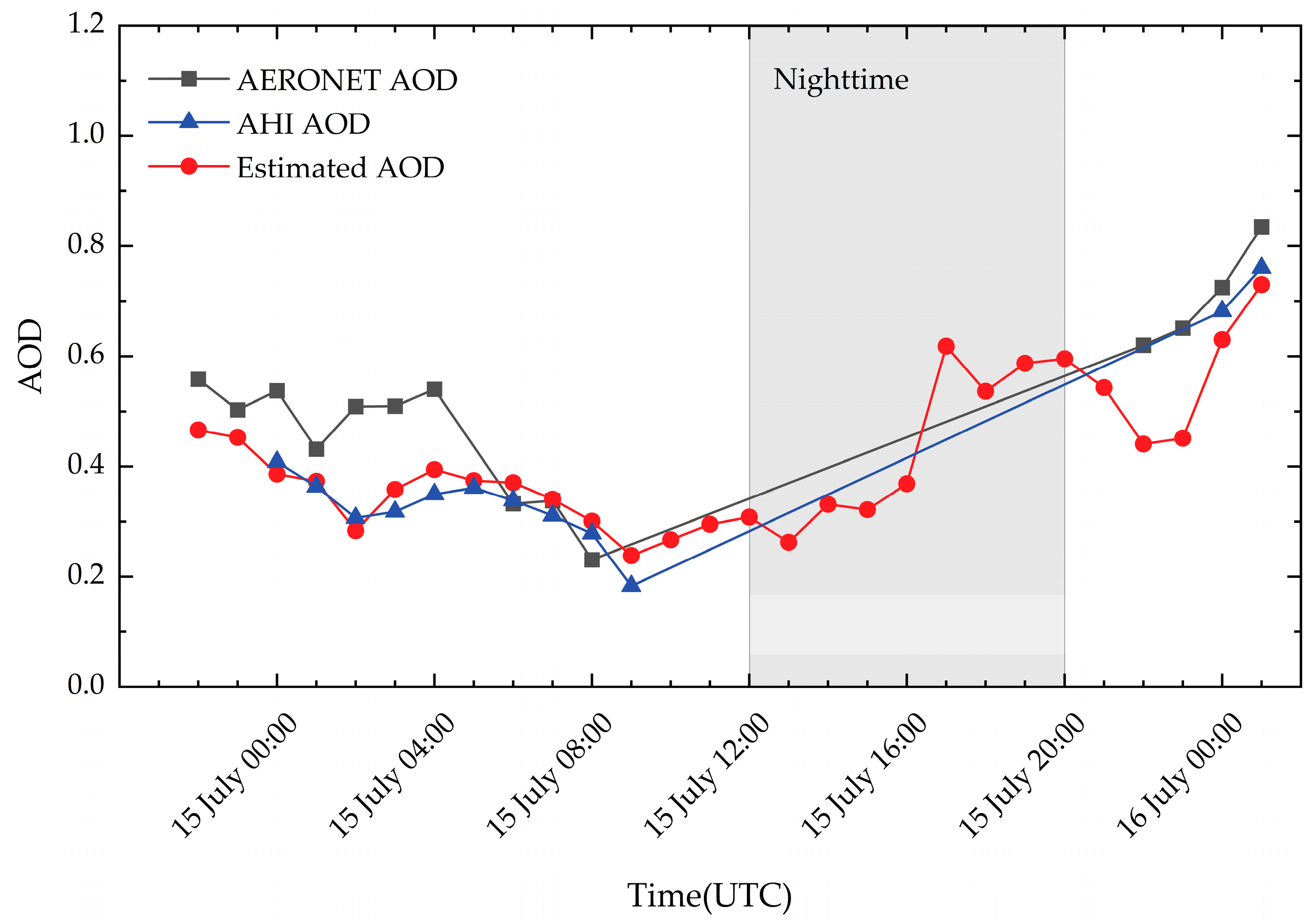
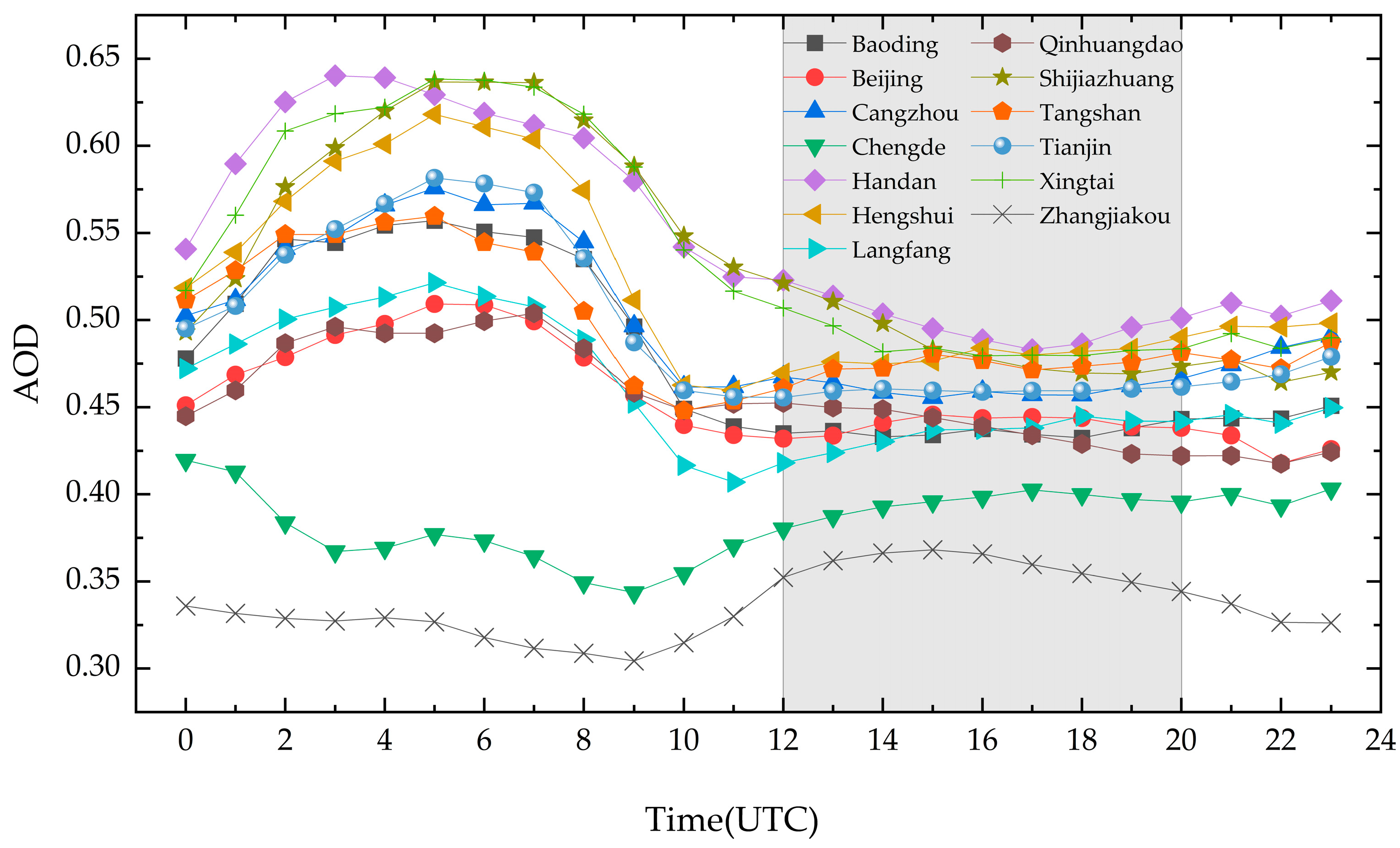
3.2.2. Comparison of Time Trends
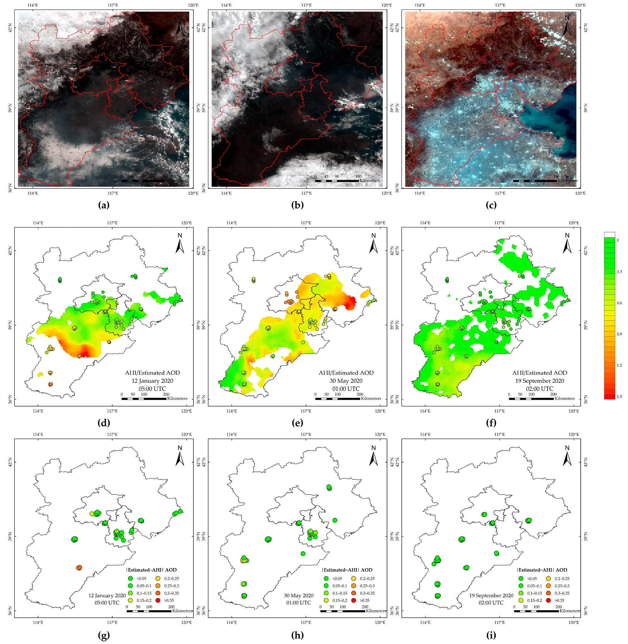
3.2.3. Comparison of Spatial Distribution
3.3. Analysis of All-Day AOD
- 1.
- Reduction in human activity, with reductions in transportation, industrial production, and other nighttime activities leading to a decrease in airborne particulate emissions.
- 2.
- Relative weakening of atmospheric turbulence during the nighttime, which slows the vertical movement of air, diminishing the diffusion and mixing of aerosols.
4. Discussion
5. Conclusions
- 1.
- The All-Day AODES achieved an R2 of 0.855, RMSE of 0.134, and slope of 0.801 based on sample–based cross–validation. Additionally, the All-Day AODES demonstrated commendable spatial extensibility based on leave–one–city cross–validation, achieving an R2 of 0.622, RMSE of 0.216, and slope of 0.621. In this study, the All-Day AODES outperformed the RF and LGBM under two different cross–validations. The All-Day AODES has a higher estimation accuracy and fitting ability, and can better capture the differences between different cities.
- 2.
- The average absolute error between the estimated and daytime AERONET AOD at the Beijing–CAMS site was 0.0537 with an Std of 0.2256; the average absolute error between the estimated and nighttime AERONET AOD at the Beijing–CAMS site was 0.0510, with an Std of 0.1927; and the average absolute error between the estimated and daytime AERONET AOD at the Xianghe site was 0.0384 with an Std of 0.2146. The average disparities between the estimated AOD and AERONET are minimal. A comparison between the estimated, AHI, and AERONET AOD showed that the average absolute errors between the estimated and AERONET AOD were smaller than those between the AHI and AERONET AOD. The estimated value was closer to the AERONET AOD than to the AHI AOD. In addition, 91% of the average absolute errors of the daytime estimated values were within the uncertainty range of the AHI AOD, 87.5% of the average absolute errors of the nighttime estimated AOD fall within the expected uncertainty range.
- 3.
- The estimated AOD of the All-Day AODES shows spatial and temporal trends similar to those of the AERONET and AHI and can more accurately reflect the nighttime AOD trend.
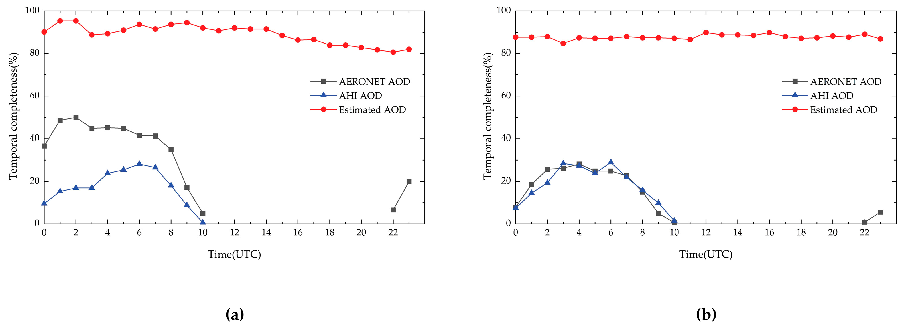
- 4.
- The All-Day AODES showed an enhanced level of temporal completeness. This compensates for the absence of satellite AOD data and furnishes hourly estimated nighttime AOD.
Author Contributions
Funding
Data Availability Statement
Acknowledgments
Conflicts of Interest
References
- Gras, J.L. AEROSOLS | Climatology of Tropospheric Aerosols. In Encyclopedia of Atmospheric Sciences; Elsevier: Amsterdam, The Netherlands, 2003; pp. 13–20. [Google Scholar]
- IPCC. Climate Change 2007: Mitigation of Climate Change; Cambridge University Press: Cambridge, UK, 2007; ISBN 978-0-511-54601-3.
- Kaufman, Y.J.; Tanré, D.; Boucher, O. A Satellite View of Aerosols in the Climate System. Nature 2002, 419, 215–223. [Google Scholar] [CrossRef] [PubMed]
- Forster, P.; Ramaswamy, V.; Artaxo, P.; Berntsen, T.; Betts, R.; Fahey, D.W.; Haywood, J.; Lean, J.; Lowe, D.C.; Myhre, G.; et al. Changes in Atmospheric Constituents and in Radiative Forcing. In Climate Change 2007: The Physical Science Basis. Contribution of Working Group I to the 4th Assessment Report of the Intergovernmental Panel on Climate Change; Solomon, S., Qin, D., Manning, M., Chen, Z., Marquis, M., Averyt, K.B., Tignor, M., Miller, H.L., Eds.; Cambridge University Press: Cambridge, UK; New York, NY, USA, 2007. [Google Scholar]
- Myhre, G. Consistency Between Satellite-Derived and Modeled Estimates of the Direct Aerosol Effect. Science 2009, 325, 187–190. [Google Scholar] [CrossRef] [PubMed]
- Wu, D.; Tie, X.; Li, C.; Ying, Z.; Kai-Hon Lau, A.; Huang, J.; Deng, X.; Bi, X. An Extremely Low Visibility Event over the Guangzhou Region: A Case Study. Atmos. Environ. 2005, 39, 6568–6577. [Google Scholar] [CrossRef]
- Moody, J.L.; Keene, W.C.; Cooper, O.R.; Voss, K.J.; Aryal, R.; Eckhardt, S.; Holben, B.; Maben, J.R.; Izaguirre, M.A.; Galloway, J.N. Flow Climatology for Physicochemical Properties of Dichotomous Aerosol over the Western North Atlantic Ocean at Bermuda. Atmos. Chem. Phys. 2014, 14, 691–717. [Google Scholar] [CrossRef]
- Tzanis, C.; Varotsos, C.; Ferm, M.; Christodoulakis, J.; Assimakopoulos, M.N.; Efthymiou, C. Nitric Acid and Particulate Matter Measurements at Athens, Greece, in Connection with Corrosion Studies. Atmos. Chem. Phys. 2009, 9, 8309–8316. [Google Scholar] [CrossRef]
- Tzanis, C.; Varotsos, C.; Christodoulakis, J.; Tidblad, J.; Ferm, M.; Ionescu, A.; Lefevre, R.-A.; Theodorakopoulou, K.; Kreislova, K. On the Corrosion and Soiling Effects on Materials by Air Pollution in Athens, Greece. Atmos. Chem. Phys. 2011, 11, 12039–12048. [Google Scholar] [CrossRef]
- Von Der Weiden-Reinmüller, S.-L.; Drewnick, F.; Crippa, M.; Prévôt, A.S.H.; Meleux, F.; Baltensperger, U.; Beekmann, M.; Borrmann, S. Application of Mobile Aerosol and Trace Gas Measurements for the Investigation of Megacity Air Pollution Emissions: The Paris Metropolitan Area. Atmos. Meas. Tech. 2014, 7, 279–299. [Google Scholar] [CrossRef]
- Al-Saadi, J.; Szykman, J.; Pierce, R.B.; Kittaka, C.; Neil, D.; Chu, D.A.; Remer, L.; Gumley, L.; Prins, E.; Weinstock, L.; et al. Improving National Air Quality Forecasts with Satellite Aerosol Observations. Bull. Am. Meteorol. Soc. 2005, 86, 1249–1262. [Google Scholar] [CrossRef]
- Ho, H.C.; Wong, M.S.; Yang, L.; Shi, W.; Yang, J.; Bilal, M.; Chan, T.-C. Spatiotemporal Influence of Temperature, Air Quality, and Urban Environment on Cause-Specific Mortality during Hazy Days. Environ. Int. 2018, 112, 10–22. [Google Scholar] [CrossRef] [PubMed]
- Mishchenko, M.I.; Geogdzhayev, I.V.; Cairns, B.; Carlson, B.E.; Chowdhary, J.; Lacis, A.A.; Liu, L.; Rossow, W.B.; Travis, L.D. Past, Present, and Future of Global Aerosol Climatologies Derived from Satellite Observations: A Perspective. J. Quant. Spectrosc. Radiat. Transf. 2007, 106, 325–347. [Google Scholar] [CrossRef]
- Varotsos, C.; Ondov, J.; Tzanis, C.; Öztürk, F.; Nelson, M.; Ke, H.; Christodoulakis, J. An Observational Study of the Atmospheric Ultra-Fine Particle Dynamics. Atmos. Environ. 2012, 59, 312–319. [Google Scholar] [CrossRef]
- Doyle, M.; Dorling, S. Satellite and Ground Based Monitoring of Aerosol Plumes. In Urban Air Quality—Recent Advances; Sokhi, R.S., Bartzis, J.G., Eds.; Springer: Dordrecht, The Netherlands, 2002; pp. 615–629. ISBN 978-94-010-3935-2. [Google Scholar]
- Barreto, Á.; Cuevas, E.; Granados-Muñoz, M.-J.; Alados-Arboledas, L.; Romero, P.M.; Gröbner, J.; Kouremeti, N.; Almansa, A.F.; Stone, T.; Toledano, C.; et al. The New Sun-Sky-Lunar Cimel CE318-T Multiband Photometer—A Comprehensive Performance Evaluation. Atmos. Meas. Tech. 2016, 9, 631–654. [Google Scholar] [CrossRef]
- De Leeuw, G.; Holzer-Popp, T.; Bevan, S.; Davies, W.H.; Descloitres, J.; Grainger, R.G.; Griesfeller, J.; Heckel, A.; Kinne, S.; Klüser, L.; et al. Evaluation of Seven European Aerosol Optical Depth Retrieval Algorithms for Climate Analysis. Remote Sens. Environ. 2015, 162, 295–315. [Google Scholar] [CrossRef]
- Li, C.F.; Dai, Y.Y.; Liu, F.; Zhao, J.J. Inversion of Aerosol Optical Depth Based on MODIS Remote Sensor. Appl. Mech. Mater. 2015, 738–739, 209–212. [Google Scholar] [CrossRef]
- Hsu, N.C.; Jeong, M.-J.; Bettenhausen, C.; Sayer, A.M.; Hansell, R.; Seftor, C.S.; Huang, J.; Tsay, S.-C. Enhanced Deep Blue Aerosol Retrieval Algorithm: The Second Generation. J. Geophys. Res. Atmos. 2013, 118, 9296–9315. [Google Scholar] [CrossRef]
- Han, J.; Tao, Z.; Xie, Y.; Li, H.; Liu, Q.; Guan, X. A Novel Radiometric Cross-Calibration of GF-6/WFV with MODIS at the Dunhuang Radiometric Calibration Site. IEEE J. Sel. Top. Appl. Earth Obs. Remote Sens. 2021, 14, 1645–1653. [Google Scholar] [CrossRef]
- Han, J.; Tao, Z.; Xie, Y.; Li, H.; Guan, X.; Yi, H.; Shi, T.; Wang, G. Radiometric Cross-Calibration of GF-6/WFV Sensor Using MODIS Images with Different BRDF Models. IEEE Trans. Geosci. Remote Sens. 2022, 60, 5409311. [Google Scholar] [CrossRef]
- Zhang, J.; Reid, J.S.; Miller, S.D.; Turk, F.J. Strategy for Studying Nocturnal Aerosol Optical Depth Using Artificial Lights. Int. J. Remote Sens. 2008, 29, 4599–4613. [Google Scholar] [CrossRef]
- Johnson, R.S.; Zhang, J.; Hyer, E.J.; Miller, S.D.; Reid, J.S. Preliminary Investigations toward Nighttime Aerosol Optical Depth Retrievals from the VIIRS Day/Night Band. Atmos. Meas. Tech. 2013, 6, 1245–1255. [Google Scholar] [CrossRef]
- Jiang, M.; Chen, L.; He, Y.; Hu, X.; Liu, M.; Zhang, P. Nighttime aerosol optical depth retrievals from VIIRS day/night band data. Natl. Remote Sens. Bull. 2022, 26, 493–504. [Google Scholar] [CrossRef]
- Li, H.; Hu, S.; Ma, S.; Tan, Z.; Ai, W.; Yan, W. Retrieving Nighttime Aerosol Optical Depth Using Combined Measurements of Satellite Low Light Channels and Ground-Based Integrating Spheres. Int. J. Remote Sens. 2022, 1–13. [Google Scholar] [CrossRef]
- Giles, D.M.; Sinyuk, A.; Sorokin, M.G.; Schafer, J.S.; Smirnov, A.; Slutsker, I.; Eck, T.F.; Holben, B.N.; Lewis, J.R.; Campbell, J.R.; et al. Advancements in the Aerosol Robotic Network (AERONET) Version 3 Database—Automated near-Real-Time Quality Control Algorithm with Improved Cloud Screening for Sun Photometer Aerosol Optical Depth (AOD) Measurements. Atmos. Meas. Tech. 2019, 12, 169–209. [Google Scholar] [CrossRef]
- Burton, S.P.; Ferrare, R.A.; Hostetler, C.A.; Hair, J.W.; Rogers, R.R.; Obland, M.D.; Butler, C.F.; Cook, A.L.; Harper, D.B.; Froyd, K.D. Aerosol Classification Using Airborne High Spectral Resolution Lidar Measurements—Methodology and Examples. Atmos. Meas. Tech. 2012, 5, 73–98. [Google Scholar] [CrossRef]
- Kolmonen, P.; Sogacheva, L.; Virtanen, T.H.; De Leeuw, G.; Kulmala, M. The ADV/ASV AATSR Aerosol Retrieval Algorithm: Current Status and Presentation of a Full-Mission AOD Dataset. Int. J. Digit. Earth 2016, 9, 545–561. [Google Scholar] [CrossRef]
- Jalal, K.A.; Asmat, A.; Ahmad, N. Aerosol Optical Depth (AOD) Retrieval Method Using MODIS. In Proceedings of the 2015 International Conference on Space Science and Communication (IconSpace), Langkawi, Malaysia, 10–12 August 2015; IEEE: Piscataway, NJ, USA, 2015; pp. 370–374. [Google Scholar]
- Miller, S.; Straka, W.; Mills, S.; Elvidge, C.; Lee, T.; Solbrig, J.; Walther, A.; Heidinger, A.; Weiss, S. Illuminating the Capabilities of the Suomi National Polar-Orbiting Partnership (NPP) Visible Infrared Imaging Radiometer Suite (VIIRS) Day/Night Band. Remote Sens. 2013, 5, 6717–6766. [Google Scholar] [CrossRef]
- Yang, F.; Wang, Y.; Tao, J.; Wang, Z.; Fan, M.; De Leeuw, G.; Chen, L. Preliminary Investigation of a New AHI Aerosol Optical Depth (AOD) Retrieval Algorithm and Evaluation with Multiple Source AOD Measurements in China. Remote Sens. 2018, 10, 748. [Google Scholar] [CrossRef]
- Kikuchi, M.; Murakami, H.; Suzuki, K.; Nagao, T.M.; Higurashi, A. Improved Hourly Estimates of Aerosol Optical Thickness Using Spatiotemporal Variability Derived From Himawari-8 Geostationary Satellite. IEEE Trans. Geosci. Remote Sens. 2018, 56, 3442–3455. [Google Scholar] [CrossRef]
- Zheng, Y.; Che, H.; Yang, L.; Chen, J.; Wang, Y.; Xia, X.; Zhao, H.; Wang, H.; Wang, D.; Gui, K.; et al. Optical and Radiative Properties of Aerosols during a Severe Haze Episode over the North China Plain in December 2016. J. Meteorol. Res. 2017, 31, 1045–1061. [Google Scholar] [CrossRef]
- Miller, S.D.; Combs, C.L.; Kidder, S.Q.; Lee, T.F. Assessing Moonlight Availability for Nighttime Environmental Applications by Low-Light Visible Polar-Orbiting Satellite Sensors. J. Atmos. Ocean. Technol. 2012, 29, 538–557. [Google Scholar] [CrossRef]
- Giles, D.M.; Slutsker, I.; Schafer, J.; Sorokin, M.G.; Smirnov, A.; Eck, T.F.; Holben, B.; Welton, E.J. Uncertainty and Bias in AERONET Nighttime AOD Measurements. In AGU Fall Meeting Abstracts; American Geophysical Union: Washington, DC, USA, 2019; Volume 2019, p. A23R-3050. [Google Scholar]
- Peng, J.; Hu, M.; Shang, D.; Wu, Z.; Du, Z.; Tan, T.; Wang, Y.; Zhang, F.; Zhang, R. Explosive Secondary Aerosol Formation during Severe Haze in the North China Plain. Environ. Sci. Technol. 2021, 55, 2189–2207. [Google Scholar] [CrossRef] [PubMed]
- Kim, K.N.; Kim, S.H.; Park, S.S.; Lee, Y.G. Feasibility Analysis of AERONET Lunar AOD for Nighttime Particulate Matter Estimation. Environ. Res. Commun. 2023, 5, 051004. [Google Scholar] [CrossRef]
- Ma, Z.; Hu, X.; Huang, L.; Bi, J.; Liu, Y. Estimating Ground-Level PM2.5 in China Using Satellite Remote Sensing. Environ. Sci. Technol. 2014, 48, 7436–7444. [Google Scholar] [CrossRef] [PubMed]
- Rohen, G.J.; Von Hoyningen-Huene, W.; Kokhanovsky, A.; Dinter, T.; Vountas, M.; Burrows, J.P. Retrieval of Aerosol Mass Load (PM10) from MERIS/Envisat Top of Atmosphere Spectral Reflectance Measurements over Germany. Atmos. Meas. Tech. 2011, 4, 523–534. [Google Scholar] [CrossRef]
- Koelemeijer, R.B.A.; Homan, C.D.; Matthijsen, J. Comparison of Spatial and Temporal Variations of Aerosol Optical Thickness and Particulate Matter over Europe. Atmos. Environ. 2006, 40, 5304–5315. [Google Scholar] [CrossRef]
- Estellés, V.; Martínez-Lozano, J.A.; Pey, J.; Sicard, M.; Querol, X.; Esteve, A.R.; Utrillas, M.P.; Sorribas, M.; Gangoiti, G.; Alastuey, A.; et al. Study of the Correlation between Columnar Aerosol Burden, Suspended Matter at Ground and Chemical Components in a Background European Environment. J. Geophys. Res. Atmos. 2012, 117, D04201. [Google Scholar] [CrossRef]
- Seo, S.; Kim, J.; Lee, H.; Jeong, U.; Kim, W.; Holben, B.N.; Kim, S.-W.; Song, C.H.; Lim, J.H. Estimation of PM10 Concentrations over Seoul Using Multiple Empirical Models with AERONET and MODIS Data Collected during the DRAGON-Asia Campaign. Atmos. Chem. Phys. 2015, 15, 319–334. [Google Scholar] [CrossRef]
- Zheng, C.; Zhao, C.; Zhu, Y.; Wang, Y.; Shi, X.; Wu, X.; Chen, T.; Wu, F.; Qiu, Y. Analysis of Influential Factors for the Relationship between PM2.5 and AOD in Beijing. Atmos. Chem. Phys. 2017, 17, 13473–13489. [Google Scholar] [CrossRef]
- Dee, D.P.; Uppala, S.M.; Simmons, A.J.; Berrisford, P.; Poli, P.; Kobayashi, S.; Andrae, U.; Balmaseda, M.A.; Balsamo, G.; Bauer, P.; et al. The ERA-Interim Reanalysis: Configuration and Performance of the Data Assimilation System. Q. J. R. Meteorol. Soc. 2011, 137, 553–597. [Google Scholar] [CrossRef]
- Fan, X.; Nie, G.; Deng, Y.; An, J.; Song, P.; Li, H.; Gu, Y. Influence of Earthquake on the Atmospheric Aerosols Study Using Aeronet Retrieved Aerosol Optical Depth. In Proceedings of the 2016 IEEE International Geoscience and Remote Sensing Symposium (IGARSS), Beijing, China, 10–15 July 2016; pp. 4080–4083. [Google Scholar]
- Fan, Z.; Zhan, Q.; Yang, C.; Liu, H.; Bilal, M. Estimating PM2.5 Concentrations Using Spatially Local Xgboost Based on Full-Covered SARA AOD at the Urban Scale. Remote Sens. 2020, 12, 3368. [Google Scholar] [CrossRef]
- Peng, J.; Han, H.; Yi, Y.; Huang, H.; Xie, L. Machine Learning and Deep Learning Modeling and Simulation for Predicting PM2.5 Concentrations. Chemosphere 2022, 308, 136353. [Google Scholar] [CrossRef]
- Zhang, J.; Zhang, H.; Wang, R.; Zhang, M.; Huang, Y.; Hu, J.; Peng, J. Measuring the Critical Influence Factors for Predicting Carbon Dioxide Emissions of Expanding Megacities by XGBoost. Atmosphere 2022, 13, 599. [Google Scholar] [CrossRef]
- Snoek, J.; Larochelle, H.; Adams, R.P. Practical Bayesian Optimization of Machine Learning Algorithms. In Proceedings of the Advances in Neural Information Processing Systems, Lake Tahoe, NV, USA, 3–6 December 2012; Curran Associates, Inc.: New York, NY, USA, 2012; Volume 25. [Google Scholar]
- Ma, Y.; Zhang, W.; Zhang, L.; Gu, X.; Yu, T. Estimation of Ground-Level PM2.5 Concentration at Night in Beijing-Tianjin-Hebei Region with NPP/VIIRS Day/Night Band. Remote Sens. 2023, 15, 825. [Google Scholar] [CrossRef]
- Ma, Y.; Zhang, W.; Chen, X.; Zhang, L.; Liu, Q. High Spatial Resolution Nighttime PM2.5 Datasets in the Beijing–Tianjin–Hebei Region from 2015 to 2021 Using VIIRS/DNB and Deep Learning Model. Remote Sens. 2023, 15, 4271. [Google Scholar] [CrossRef]
- Wei, J.; Huang, W.; Li, Z.; Xue, W.; Peng, Y.; Sun, L.; Cribb, M. Estimating 1-Km-Resolution PM2.5 Concentrations across China Using the Space-Time Random Forest Approach. Remote Sens. Environ. 2019, 231, 111221. [Google Scholar] [CrossRef]
- Ma, J.; Zhang, R.; Xu, J.; Yu, Z. MERRA-2 PM2.5 Mass Concentration Reconstruction in China Mainland Based on LightGBM Machine Learning. Sci. Total Environ. 2022, 827, 154363. [Google Scholar] [CrossRef] [PubMed]
- Zhang, W.; Gu, X.; Xu, H.; Yu, T.; Zheng, F. Assessment of OMI near-UV Aerosol Optical Depth over Central and East Asia. J. Geophys. Res. Atmos. 2016, 121, 382–398. [Google Scholar] [CrossRef]
- Zhang, W.; Xu, H.; Zheng, F. Aerosol Optical Depth Retrieval over East Asia Using Himawari-8/AHI Data. Remote Sens. 2018, 10, 137. [Google Scholar] [CrossRef]
- Zhang, W.; Xu, H.; Zhang, L. Assessment of Himawari-8 AHI Aerosol Optical Depth Over Land. Remote Sens. 2019, 11, 1108. [Google Scholar] [CrossRef]
- Sun, L.; Li, R.-B.; Tian, X.-P.; Wei, J. Analysis of the Temporal and Spatial Variation of Aerosols in the Beijing-Tianjin-Hebei Region with a 1 Km AOD Product. Aerosol Air Qual. Res. 2017, 17, 923–935. [Google Scholar] [CrossRef]


| Site | Latitude/°N | Longitude/°E |
|---|---|---|
| XiangHe | 39.754 | 116.962 |
| Beijing–CAMS | 39.933 | 116.317 |
| Category | Variable | Content | Units | Spatial Resolution | Temporal Resolution |
|---|---|---|---|---|---|
| Ground air quality data | PM2.5 | Particulate matter ≤ 2.5 μm 1 h average | μg/m3 | site | Hourly |
| PM10 | Particulate matter ≤ 10 μm 1 h average | μg/m3 | site | Hourly | |
| SO2 | SO2 1 h average | μg/m3 | site | Hourly | |
| NO2 | NO2 1 h average | μg/m3 | site | Hourly | |
| O3 | O3 1 h average | μg/m3 | site | Hourly | |
| Meteorological data | BLH | Boundary layer height | m | 0.25° × 0.25° | Hourly |
| SP | Surface pressure | Pa | 0.25° × 0.25° | Hourly | |
| T2M | 2 m temperature | K | 0.25° × 0.25° | Hourly | |
| U10 | 10 m u–component of wind | m/s | 0.25° × 0.25° | Hourly | |
| V10 | 10 m v–component of wind | m/s | 0.25° × 0.25° | Hourly | |
| RH | Relative humidity | % | 0.25° × 0.25° | Hourly | |
| Satellite AOD data | AOD | Aerosol Optical Depth | – | 0.05° × 0.05° | Hourly |
| Model | Parameter | Meaning | Value |
|---|---|---|---|
| All-Day AODES | n_estimators | Number of trees | 731 |
| max_depth | Maximum tree depth | 41 | |
| min_child_weight | Minimum sample weight sum in child nodes | 38.66 | |
| learning_rate | Learning rate | 0.031 |
| Variable | AHI AOD | ||
|---|---|---|---|
| Slope | Intercept | Correlation Coefficient | |
| PM2.5 | 0.006 | 0.24 | 0.598 |
| PM10 | 0.003 | 0.217 | 0.533 |
| SO2 | 0.007 | 0.373 | 0.259 |
| NO2 | 0.008 | 0.274 | 0.424 |
| O3 | 1.29 × 10⁻⁴ | 0.454 | 0.018 |
| BLH | −1.33 × 10⁻⁴ | 0.627 | −0.303 |
| SP | 1.01 × 10⁻⁵ | −0.539 | 0.097 |
| T2M | 0.004 | −0.591 | 0.101 |
| U10 | −0.04 | 0.497 | −0.238 |
| V10 | 0.037 | 0.464 | 0.263 |
| RH | 0.008 | 0.189 | 0.388 |
| Model | Parameter | Meaning | Value |
|---|---|---|---|
| RF | n_estimators | Number of trees | 429 |
| max_depth | Maximum tree depth | 30 | |
| max_features | Maximum number of features | 0.691 | |
| min_samples_split | Minimum number of samples required for internal node redistribution | 4 | |
| LGBM | n_estimators | Number of trees | 967 |
| max_depth | Maximum tree depth | 41 | |
| num_leaves | Number of leaf nodes on a tree | 29 | |
| learning_rate | Learning rate | 0.119 |
| RF | LGBM | All-Day AODES | |
|---|---|---|---|
| R2 > 0.65 | 19 | 21 | 27 |
| RMSE < 0.2 | 17 | 18 | 22 |
Disclaimer/Publisher’s Note: The statements, opinions and data contained in all publications are solely those of the individual author(s) and contributor(s) and not of MDPI and/or the editor(s). MDPI and/or the editor(s) disclaim responsibility for any injury to people or property resulting from any ideas, methods, instructions or products referred to in the content. |
© 2024 by the authors. Licensee MDPI, Basel, Switzerland. This article is an open access article distributed under the terms and conditions of the Creative Commons Attribution (CC BY) license (https://creativecommons.org/licenses/by/4.0/).
Share and Cite
Zhang, W.; Liu, S.; Chen, X.; Mi, X.; Gu, X.; Yu, T. Estimation of All-Day Aerosol Optical Depth in the Beijing–Tianjin–Hebei Region Using Ground Air Quality Data. Remote Sens. 2024, 16, 1410. https://doi.org/10.3390/rs16081410
Zhang W, Liu S, Chen X, Mi X, Gu X, Yu T. Estimation of All-Day Aerosol Optical Depth in the Beijing–Tianjin–Hebei Region Using Ground Air Quality Data. Remote Sensing. 2024; 16(8):1410. https://doi.org/10.3390/rs16081410
Chicago/Turabian StyleZhang, Wenhao, Sijia Liu, Xiaoyang Chen, Xiaofei Mi, Xingfa Gu, and Tao Yu. 2024. "Estimation of All-Day Aerosol Optical Depth in the Beijing–Tianjin–Hebei Region Using Ground Air Quality Data" Remote Sensing 16, no. 8: 1410. https://doi.org/10.3390/rs16081410
APA StyleZhang, W., Liu, S., Chen, X., Mi, X., Gu, X., & Yu, T. (2024). Estimation of All-Day Aerosol Optical Depth in the Beijing–Tianjin–Hebei Region Using Ground Air Quality Data. Remote Sensing, 16(8), 1410. https://doi.org/10.3390/rs16081410