A Bayesian Approach for Forecasting the Probability of Large Earthquakes Using Thermal Anomalies from Satellite Observations

Abstract

Studies have demonstrated the potential of satellite thermal infrared observations to detect anomalous signals preceding large earthquakes. However, the lack of well-defined precursory characteristics and inherent complexity and stochasticity of the seismicity continue to impede robust earthquake forecasts. This study investigates the potential of pre-seismic thermal anomalies, derived from five satellite-based geophysical parameters, i.e., skin temperature, air temperature, total integrated column water vapor burden, outgoing longwave radiation (OLR), and clear-sky OLR, as valuable indicators for global earthquake forecasts. We employed a spatially self-adaptive multiparametric anomaly identification scheme to refine these anomalies, and then estimated the posterior probability of an earthquake occurrence given observed anomalies within a Bayesian framework. Our findings reveal a promising link between thermal signatures and global seismicity, with elevated forecast probabilities exceeding 0.1 and significant probability gains in some strong earthquake-prone regions. A time series analysis indicates probability stabilization after approximately six years. While no single parameter consistently dominates, each contributes precursory information, suggesting a promising avenue for a multi-parametric approach. Furthermore, novel anomaly indices incorporating probabilistic information significantly reduce false alarms and improve anomaly recognition. Despite remaining challenges in developing dynamic short-term probabilities, rigorously testing detection algorithms, and improving ensemble forecast strategies, this study provides compelling evidence for the potential of thermal anomalies to play a key role in global earthquake forecasts. The ability to reliably estimate earthquake forecast probabilities, given the ever-present threat of destructive earthquakes, holds considerable societal and ecological importance for mitigating earthquake risk and improving preparedness strategies.

1. Introduction

While deterministic earthquake prediction remains in its nascent stages and its foreseeable success is uncertain [1,2], increasing efforts are focused on developing reliable earthquake forecasts to facilitate community preparedness and potentially mitigate damage and casualties. The probabilistic forecast of large earthquakes, following the recognition of pre-earthquake anomalies, is a crucial step in advancing the implementation of operational earthquake forecasting (OEF) systems. Seismicity data serve as the primary driver for OEF systems, enabling timely forecasts that can help mitigate earthquake risk during earthquake sequences [3]. However, integrating thermal anomalies detected by satellite measurements into OEF systems remains challenging, despite their potential to signal the occurrence of strong earthquakes.

Pre-seismic thermal anomalies have emerged as potential seismic precursors for upcoming strong earthquakes [4,5]. Decades of research spanning various earthquakes and geographic regions have investigated diverse anomalous phenomena using geophysical and geochemical parameters, such as outgoing longwave radiation (OLR), skin and air temperature, and atmospheric water vapor, suggesting their possible connection to seismic activity [6,7,8,9]. While researchers have reported encouraging findings regarding the detection of anomalous signals from space potentially correlated with strong earthquakes, these results remain subject to debate and criticism [1,10,11]. A critical challenge lies in the lack of universally identifiable and diagnostic pre-seismic anomaly characteristics or a “fingerprint” that reliably predicts large earthquakes [12,13]. This limitation, further supported by studies on the statistical correlation between pre-seismic anomalies and earthquakes [14,15,16], hinders the integration of these anomalies into OEF systems due to high false-alarm rates from the prevalence of spatially and temporally scattered anomalous fluctuations [17]. While statistically robust pre-seismic anomaly detection will remain a significant challenge in the near future, the immediate need for earthquake forecast support to mitigate the economic and human toll of strong earthquakes underscores the urgency of exploring alternative avenues.

Given the limitations of pre-seismic anomaly identification, coupled with a growing consensus towards probabilistic earthquake forecasts [17,18], estimating the conditional probability of earthquakes upon detected thermal anomalies appears to be a more promising approach. This probabilistic framework can inherently account for the uncertainties associated with the non-uniqueness of current anomaly recognitions. Existing probabilistic forecast methods often utilize geodetic and seismological data. Jackson and Kagan [19] employed the rate-density function solely from earthquake catalogs. Petersen, et al. [20] built a time-independent probability model assuming a Poisson distribution for earthquake occurrences. By leveraging earthquake catalogs, a Poisson probability was calculated, successfully revealing an 82% likelihood of a 7.7 Mw earthquake in the Colima region characterized by a low b-value [21]. Shen, et al. [18] proposed a probabilistic forecast approach using a tapered Gutenberg–Richter magnitude distribution, based on the crustal strain rate, for the intermediate-term periods between large earthquakes. Notably, the Third Uniform California Earthquake Rupture Forecast (UCERF3) exemplifies a successful implementation of a probabilistic forecast by synthesizing seismic, geologic, and geodetic data [22]. The integration of thermal anomalies has the potential to further enhance short-term forecasting capabilities. Fidani [17] and Fidani, et al. [23] proposed an approach to estimate the conditional probability of an earthquake occurrence for a short-term forecast based on the relationship between covariance and cross-correlation, applied to CO₂ and electron burst anomalies. However, such methods remain reliant on certain modeling assumptions and have not yet fully demonstrated their predictive power for earthquake forecast probability ($P_{EQ}$) at a global scale. Current probabilistic forecast methods predominantly leverage regional geologic, geodetic, and seismological data, typically employing empirical statistical models. However, these models possess inherent constraints in comprehensively capturing the intricate physical mechanisms underlying earthquake occurrences. Unlike deterministic models that presuppose a direct causal link between observed anomalies and imminent seismic events, the Bayesian framework presents a promising approach for augmenting earthquake forecasting proficiency. By facilitating the assimilation of prior knowledge and iterative refinement of probability assessments with the incorporation of new data, Bayesian methods offer a pathway towards improved forecasting accuracy.

Driven by its strengths in probabilistic inference, Bayesian probability theory is gaining considerable traction in earthquake science for tackling complex models. By synergistically integrating historical seismic data, geological information, and real-time monitoring data, Bayesian models refine earthquake probability estimates and illuminate the intricate interplay between stress accumulation, fault geometry, and seismic release [24]. Notably, the Bayesian approach has been applied in various contexts within earthquake forecasts. Marzocchi, et al. [25] utilized it for the model comparison of earthquake forecast approaches based on Bayes factors. Darzi, et al. [26] employed a Bayesian spatiotemporal Epidemic-Type Aftershock Sequence (ETAS) clustering model to forecast aftershocks following the 2008 Mw6.3 Ölfus earthquake in Iceland. Dong, et al. [27] leveraged the Bayesian predictive distribution to account for parameter uncertainties in both the ETAS model and modified Omori law models, ultimately comparing their forecast skills. Particularly, the studies support the superiority of Bayesian probability theory over null hypothesis testing in estimating the conditional probability of earthquake occurrences [10,25]. Null hypothesis testing is a statistical technique utilized to assess the validity of a hypothesis ${\mathrm{H}}_0$ by contrasting it with an alternative hypothesis ${\mathrm{H}}_1$. ${\mathrm{H}}_0$ denotes the absence of an effect, relationship, or group disparity, while ${\mathrm{H}}_1$ suggests their presence. Researchers analyze data to determine if observed results exhibit statistical significance or could have occurred by chance, assuming ${\mathrm{H}}_0$ is true. This involves calculating a test statistic and determining the probability of obtaining extreme results given ${\mathrm{H}}_0$. If this probability, the p-value, falls below a predetermined threshold, typically 0.05, ${\mathrm{H}}_0$ is rejected in favor of ${\mathrm{H}}_1$. It is clear that Bayesian inference plays a critical role in deciphering the intricate dynamics of fault systems and predicting seismic events, empowering us to deliver more reliable earthquake forecasts and formulate effective mitigation strategies. In this context, satellite data present a wealth of observational data for past seismic cases, enabling robust statistical analyses aimed at characterizing the $P_{EQ}$ of thermal anomalies. Such analyses are particularly valuable for comparing the performance of multiple forecast models and advancing the development of OEF systems.

This study utilizes five geophysical parameters retrieved from the Atmospheric Infrared Sounder (AIRS) product to estimate the posterior probability of an earthquake occurrence (also known as $P_{EQ}$) within seismically active regions globally, without requiring additional hypotheses. Leveraging a self-adaptive multiparametric anomaly identification scheme, we extract seismic-related anomalies from historical data, serving as the foundation for subsequent probability estimation. A Bayesian framework is then employed to calculate $P_{EQ}$ relying on identified anomalies from each parameter alongside earthquake data. This research represents a potential pioneering study in utilizing thermal anomalies derived from satellite observations to forecast large earthquakes, with our findings demonstrating promising preliminary evidence for their significance in indicating upcoming strong seismic events. Furthermore, the estimated $P_{EQ}$ can serve as valuable prior knowledge for subsequent monitoring and a comparative analysis of precursory anomalies. Derived from historical earthquake catalogs and nearly two decades of remote sensing data, $P_{EQ}$ represents a long-term average condition regarding earthquake occurrences and their correlations with triggered anomalous phenomena. They also offer quantitative indicators, critical for decision making by responsible authorities regarding potential future earthquakes and enhancing seismic regime prediction capabilities.

2. Study Area and Data

2.1. Global Seismically Active Regions

Unlike randomly distributed phenomena, strong earthquakes exhibit a non-random spatial distribution, predominantly clustering along major fault systems [28]. While their timing remains largely stochastic [29], analyzing their spatial patterns can provide valuable insights into future seismicity. To define seismically active regions for this study (Figure 1), we utilized an earthquake catalog from the United States Geological Survey (USGS) comprising 4719 events with magnitudes ≥ 6 and focal depths ≤ 70 km recorded between 1980 and 2020. A 1° × 1° grid was overlaid on the globe, and the number of earthquakes within each grid cell was searched based on their latitude and longitude. Grid cells exceeding a threshold count of 1 were retained as seismically active regions. For a cell containing more than one earthquake, a 5° × 5° buffer zone (shown in gray in Figure 1) was created surrounding this central cell, and the same procedure was repeated to identify the most earthquake-prone areas globally. The most tectonically active regions, with earthquake counts exceeding 20 within individual 1° × 1° grid cells, are primarily observed along major plate boundaries and mid-ocean ridges. These areas are characterized by intense plate movements and increased seismic and volcanic activities [30]. Given the reasonable assumption that historical seismic activity can inform future seismicity with similar magnitudes within adjacent regions [22], these seismically active areas were chosen as the focus of our study.

It is essential to acknowledge that the definition of globally seismically active regions relies on the prevalence of anomaly phenomena, given the constraints of utilized geophysical parameters and anomaly detection methods. This often results in a high false-alarm ratio in earthquake forecasts [31]. Many regions exhibit minimal occurrences of strong earthquakes based on historical seismic data and regional tectonic settings. Therefore, anomalies detected in these areas hardly signify impending earthquakes but could be attributed to other environmental or anthropogenic factors. Excluding such areas from consideration enhances the efficacy of earthquake forecasts, which is the primary purpose for such treatment. However, advancements in anomaly detection methods offer hope for refining the identification of relevant anomalies. A synthetic earthquake method has been devised to assess anomaly detection under such circumstances [29], indicating a long way to enhancing our understanding of pre-earthquake anomalies.

2.2. AIRS Dataset

Hyperspectral infrared (HIR) sounders are instruments that observe earth’s atmosphere and surface by capturing infrared radiation emitted by the earth across a wide range of wavelengths, typically spanning from 3 to 16 μm. By dividing the infrared spectrum into numerous narrow spectral bands, HIR sounders can provide detailed information about various atmospheric and surface properties. These properties include atmospheric temperature, water vapor content, cloud characteristics, trace gases, and other geophysical parameters. The measurements obtained by these sounders, which operate aboard satellite platforms, enable scientists to monitor and analyze atmospheric dynamics, climate patterns, weather phenomena, and environmental changes. Therefore, HIR techniques play a crucial role in advancing our understanding of earth’s climate system and improving weather forecasting capabilities. Currently, there are several operational HIR sounders, including the High-resolution Infrared Radiation Sounder (HIRS/4), the Infrared Atmospheric Sounding Interferometer (IASI), and the Cross-track Infrared Sounder (CrIS). In this study, we utilize data products from the AIRS instrument.

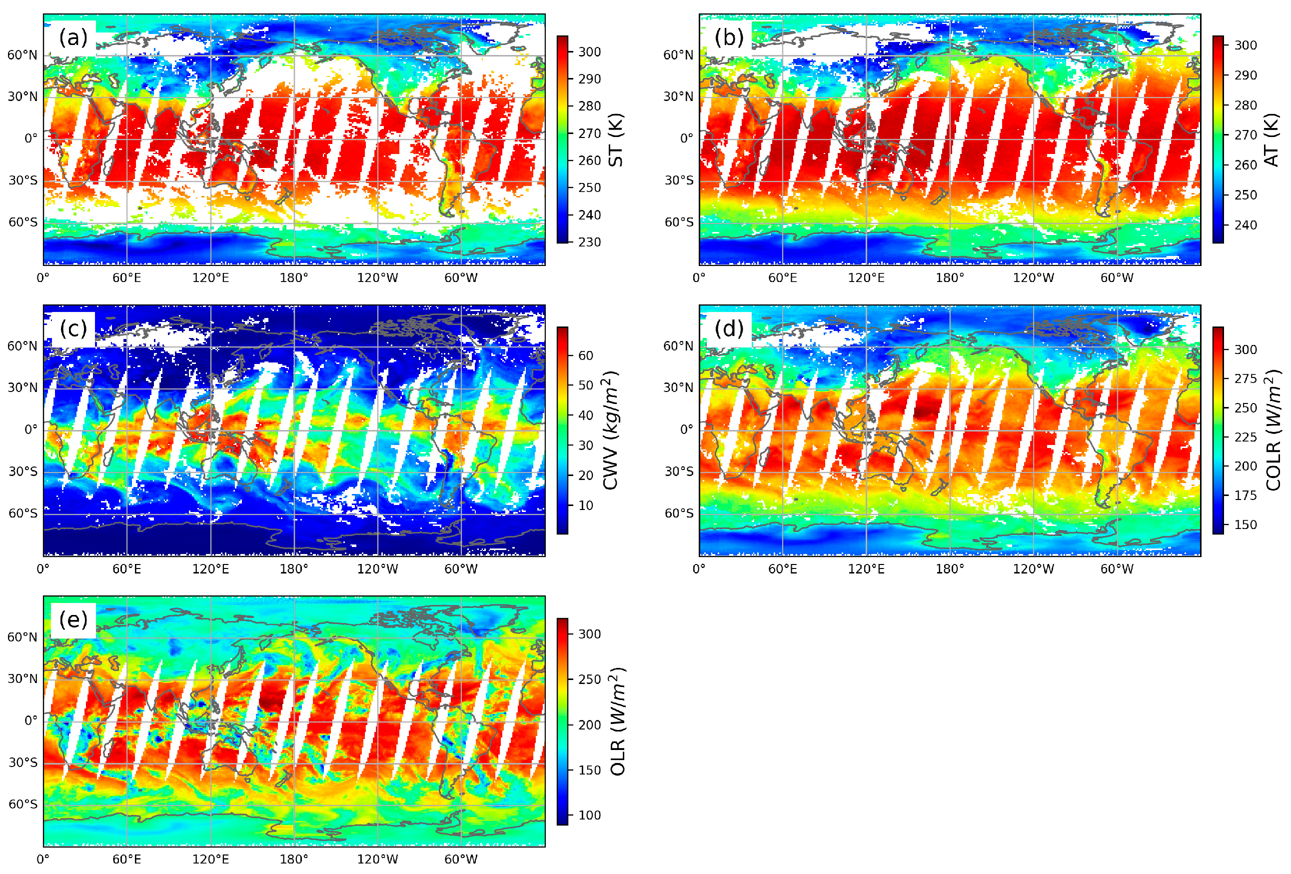
Launched on 4 May 2002, AIRS aboard the Aqua satellite represents a new generation of high-resolution infrared sounders. The instrument continuously monitors the earth–atmosphere system by observing its emitted infrared radiation with 2378 channels across a spectral range of 3.74–15.4 µm. It has a horizontal spatial resolution of 13.5 km at nadir and achieves twice-daily global coverage [32]. A key advantage of this hyperspectral technology lies in its ability to simultaneously retrieve multiple geophysical and geochemical parameters with good accuracy. This study leverages the AIRS/Aqua L3 daily standard physical retrieval (AIRS3STD) V7.0 product for night-time data to compute pre-seismic multiparametric anomalies. Offering a spatial resolution of 1° and a temporal resolution of 12 h, this product provides access to five key geophysical parameters: skin temperature (ST; K), air temperature (AT; K), total integrated column water vapor burden (CWV; kg/m²), OLR (W/m²), and clear-sky OLR (COLR; W/m²). An example of the AIRS data product is illustrated in Figure 2, where the white areas indicate missing data.

3. Methods

3.1. Pre-Seismic Anomaly Recognition

The anomalous fluctuations of the five geophysical parameters are quantified using the z-score (ZS) normalization method, expressed as

$$ZS\left(x,y,t\right)=\frac{v\left(x,y,t\right)-\mu (x,y)}{\delta (x,y)},$$

(1)

where $v\left(x,y,t\right)$ represents the current value of a given parameter at a specific location $\left(x,y\right)$ and time t; $\mu (x,y)$ and $\delta \left(x,y\right)$ denote the long-term average and standard deviation, respectively, of the reference field calculated at the same or similar time intervals over multiple years at location $\left(x,y\right)$. Anomaly detection involves identifying deviations from the normal or long-term average reference values of specific parameters within a spatial or temporal domain. These deviations serve as indicators of potential pre-seismic anomalies, partly triggered by seismogenic processes. The anomalies computed in Equation (1) hold significance only when δ(x, y) is non-zero. Considering an anomaly occurrence as a normal distribution, $ZS\left(x,y,t\right)$ with values of 1, 2, and 3 corresponds to probabilities of 68.17%, 99.45%, and 99.73%, respectively. Larger anomalies indicate a higher probability of rare events. Alternatively, the disparity between $v\left(x,y,t\right)$ and $\mu (x,y)$ of the reference field indicates the signal, while $\delta \left(x,y\right)$ of the reference field denotes the noise. A higher signal-to-noise ratio augments the likelihood of anomalies preceding an earthquake.

While the ZS method offers a quantitative measure of deviation from the background, solely relying on their values is insufficient for associating them with imminent earthquakes. In response, we developed a spatially self-adaptive multiparametric anomaly identification scheme to optimize anomaly recognition criteria for each pixel within remotely sensed data [14]. The construction of this scheme involves several key steps. Firstly, night-time data of multiparameter anomalies within a 7° × 7° sliding window for a single day are extracted from the specific period, forming a spatiotemporal data cube for the central pixel. Secondly, the potential values of four parameters are iteratively applied to the data cube, and the combination yielding the highest Matthew’s correlation coefficient (MCC) value is chosen as the optimal parameters for that pixel. These parameters include the temporal span for forecasting impending earthquakes before the current day, the absolute anomaly value of a pixel, the count of valid anomaly pixels in the neighboring window, and the number of valid days satisfying the aforementioned conditions within an observation period (e.g., 90 days). Subsequently, the computations are executed for each pixel via the sliding window, and optimal parameters are gridded to depict their spatial distributions across the entire domain. This dynamic adjustment process enhances the accuracy of identifying pre-seismic anomalies, thus improving the overall reliability of earthquake forecasts. Continuously learning from new seismic events and anomalies, the spatially adaptive approach updates the anomaly recognition criteria to adapt to evolving seismic patterns, thereby advancing forecasting capabilities on a global scale. For further details on the implementation of this scheme, please refer to Jiao, et al. [14]. These criteria serve to refine pre-earthquake anomalies by filtering the spatiotemporal data cube of ZS-based anomalies.

Earthquake forecasts are typically presented as the expected number of earthquakes within multidimensional bins, where each bin represents an interval in space, time, and magnitude [33]. This study focuses on a specific application of this framework within the context of operational forecast practices. Monthly reporting is customary, with a focus on stronger earthquakes, prompting the stipulation of a minimized spatial forecasting range. Hence, we employ a fixed spatial and temporal domain, encompassing a 7° × 7° window and forecasting earthquakes with magnitudes exceeding 6.0 within the upcoming 30 days. The observation period of satellite data used for forecasts can vary from 30 to 180 days [14], depending on the specific location and optimal parameters determined through the aforementioned procedures. These empirical values are adjustable as needed, with their forecasting efficacy warranting further scrutiny.

3.2. Earthquake Forecast Probability Based on Bayesian Theory

Effectively testing anomaly detection methods necessitates an inclusion of posterior probability that goes beyond the traditional time–location–magnitude framework of earthquake predictions [10]. Traditional earthquake prediction resembles binary classification, addressing the presence or absence of earthquakes under specific conditions. Similar to weather forecasts, earthquake forecasts provide a probability of occurrences rather than guaranteeing impending earthquakes, aligning with our limited understanding of earthquake precursory mechanisms. This transition enables the integration of more sophisticated mathematical methodologies to depict complex seismic phenomena, enhancing our ability to discern pre-earthquake anomalies continually.

For this purpose, the posterior probability of an earthquake occurrence emerges as a valuable metric, allowing for a statistical analysis based on historical seismic data, and identifying potential correlations between anomalies and past earthquakes [17]. Bayesian theory provides a powerful statistical framework for reasoning and decision making under uncertainty. Its core principle lies in iteratively updating the probability of a hypothesis based on new evidence. This enables us to seamlessly integrate prior knowledge with observed data, culminating in a posterior probability distribution. Notably, it distinguishes itself from classical frequency-based interpretations by treating probability as a measure of belief or certainty, thereby facilitating probabilistic statements about unknown parameters. Consequently, Bayesian statistics contributes to the refinement of probability estimates for seismic events, empowering more informed decision making for risk mitigation and preparedness strategies.

Within the Bayesian framework, the posterior probability of earthquake occurrences, $P\left(EQ|Ano\right)$, conditioned on the observed anomalies, can be derived for earthquake forecast estimation:

$$P\left(EQ|Ano\right)=\frac{P\left(EQ\right)P\left(Ano|EQ\right)}{P\left(Ano\right)},$$

(2)

where $P\left(EQ\right)$ is the natural probability of earthquake occurrences, also known as the a priori probability, representing our initial belief before considering the anomalies. $P\left(Ano|EQ\right)$ is the likelihood probability, representing the probability of observing the anomalies if an earthquake is to occur. $P\left(Ano\right)$ is the marginal probability of observing the anomalies, regardless of whether an earthquake occurs or not. Equation (3) further expands the marginal term $P\left(Ano\right)$ into its constituent components:

$$P\left(Ano\right)=P\left(Ano|EQ\right)P\left(EQ\right)+P\left(Ano|\overline{EQ}\right)P\left(\overline{EQ}\right),$$

(3)

where $P\left(\overline{EQ}\right)=1-P\left(EQ\right)$; and $P\left(Ano|\overline{EQ}\right)$ is the conditional probability of anomaly occurrences without earthquakes. Therefore, estimating $P\left(EQ|Ano\right)$ requires determining three key components: $P\left(EQ\right)$, $P\left(Ano|EQ\right)$, and $P\left(Ano|\overline{EQ}\right)$. This entails the careful consideration of both prior knowledge and observed data within the Bayesian framework for robust earthquake forecasts.

The $P\left(EQ\right)$ is derived from a comprehensive historical earthquake catalog provided by the USGS. This catalog comprises earthquakes with magnitudes ≥ 6.0 and focal depths < 70 km, recorded between 1900 and 2020. Each earthquake’s location is represented as a point in a two-dimensional Cartesian coordinate system with the latitude and longitude. The point data within this catalog are subsequently gridded onto a global grid with a resolution of 1° × 1° (yielding 180 × 360 pixels) for each day. For a day, we search for earthquakes occurring within a 7° × 7° neighboring window around a pixel in a 30-day forecast period. If one or more earthquakes are found within this spatiotemporal window, we consider an earthquake event to have occurred at that pixel for this day. This procedure is repeated for all pixels on this day, resulting in a grid containing cells with a value of 1 for earthquakes and 0 for no earthquakes. By this method, a daily grid is generated from 1900 to 2020. The average of all grids from 1900 to the current day yields the $P\left(EQ\right)$ grid for the current day. The resulting value represents the estimated probability of a seismic event occurring within its designated 7° × 7° spatial window and 30-day temporal window.

Following the same procedure employed for estimating $P\left(EQ\right)$, the $P\left(Ano|EQ\right)$ and $P\left(Ano|\overline{EQ}\right)$ can be concurrently calculated. The anomaly itself is derived from the methodology presented in Section 3.1. Specifically, the earthquake catalog comprises 1825 earthquakes with magnitudes ≥ 6 and focal depths ≤ 70 km, recorded between 2006 and 2020. Accordingly, the satellite data from AIRS spanning 2002 to 2020 are used to compute daily anomalies for the five relevant parameters.

The probability gain ($G_{EQ}$) is defined as the ratio between $P\left(EQ|Ano\right)$ and $P\left(EQ\right)$, quantifying the increase in earthquake probability conferred by the observed anomaly [17,34]. A robust earthquake forecast aims to simultaneously maximize the success rate and minimize false alarms, ultimately maximizing $G_{EQ}$ [10]. In addition, the MCC offers a stringent metric for evaluating forecast robustness, further supporting the maximization of $G_{EQ}$ [14]. A $G_{EQ}$ value exceeding 1 indicates that the observed anomaly likely carries precursory information within the seismogenic phase. Notably, higher $G_{EQ}$ values of anomalies for geophysical parameters suggest the increased effectiveness of their $P_{EQ}$ values in pinpointing impending large earthquakes.

4. Results

4.1. Global Probability of Earthquake Forecasting

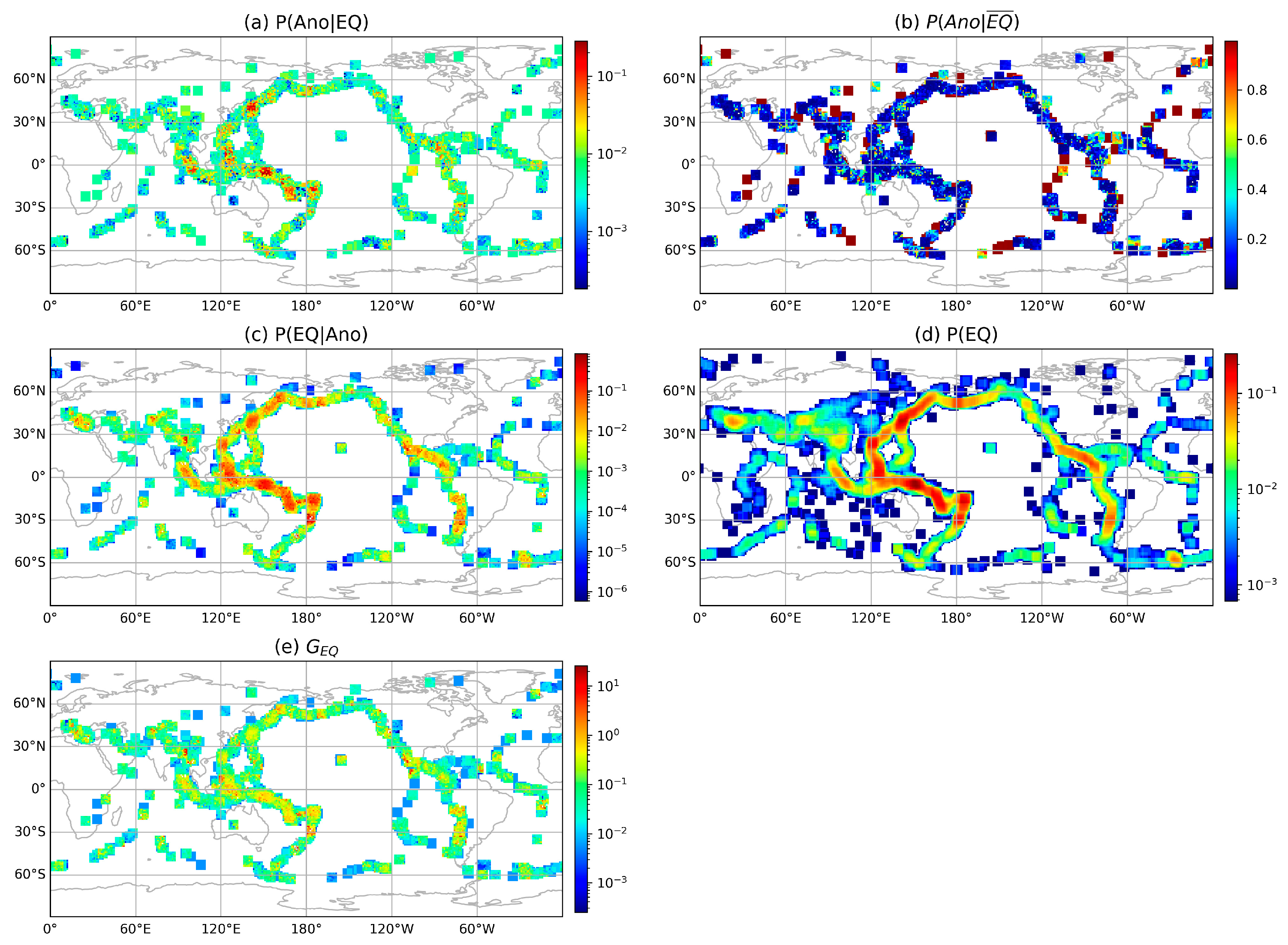
Figure 3 depicts the global $P_{EQ}$ on 31 December 2020, based on AIRS OLR anomalies, including three components used in the Bayesian formula for probability calculation. $P\left(Ano|EQ\right)$ remains consistently below 0.25 globally, and yet exhibits higher values along seismically prone regions (Figure 3a), demonstrating a clear spatial correlation. $P\left(Ano|\overline{EQ}\right)$, on the other hand, can reach values greater than 0.6, indicating a widespread prevalence of anomalous fluctuations (Figure 3b) and consequently yielding a significantly elevated false-alarm ratio for earthquake forecasting. They can serve as the quantitative indicator of the statistical significance between pre-seismic anomalies and future earthquakes: a higher $P\left(Ano|EQ\right)$ compared to $P\left(Ano|\overline{EQ}\right)$ potentially enhances forecast capacity. Figure 3c shows $P\left(EQ|Ano\right)$, with prominent global seismically active areas displaying values exceeding 0.01, albeit not surpassing 0.2. Regions such as western China and Southeast Asia exhibit elevated probabilities, suggesting an increased likelihood of forecasting imminent strong earthquakes when thermal anomalies occur. These areas align with the distribution of $P\left(EQ\right)$ presented in Figure 3d, where the circum-Pacific and Alpide seismic belts demonstrate considerably higher values. Consequently, anomalous phenomena are more likely to appear in these regions, as evidenced by Figure 3a. Crucially, Figure 3e highlights that recognized anomalies provide predictive information about earthquake preparation only when the $G_{EQ}$ exceeds 1. This indicates a heightened chance of imminent earthquakes when anomalies are observed. In fact, $G_{EQ}$ > 1 supports the overall validity of the model’s predictions [10]. Similar spatial distributions with higher probabilities in earthquake-prone areas are also observed for ST, AT, CWV, and COLR anomalies (Figures S1–S4). However, subtle variations in these distributions across different parameters emphasize their unique contributions to the characterization of pre-seismic anomalies.

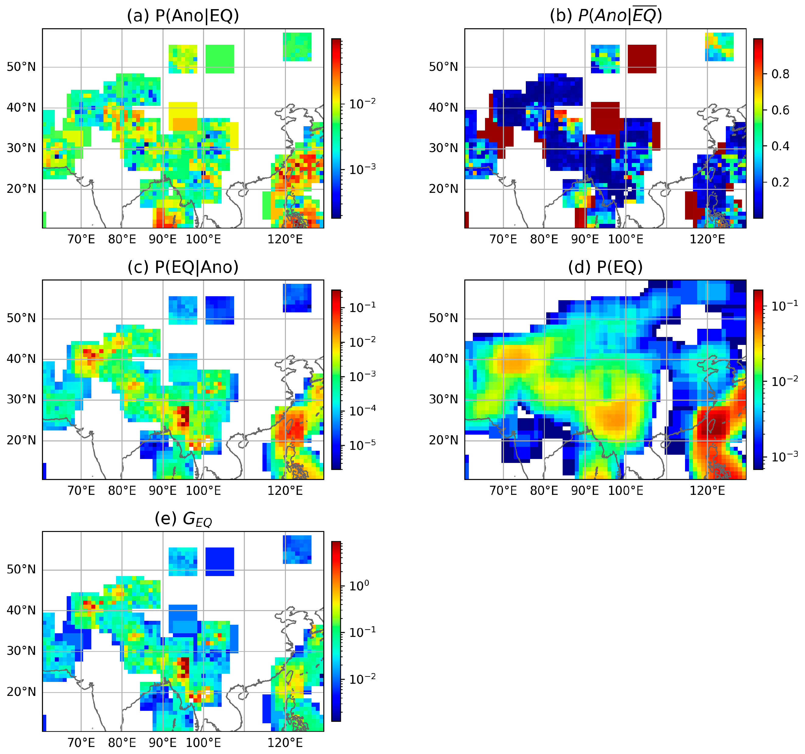
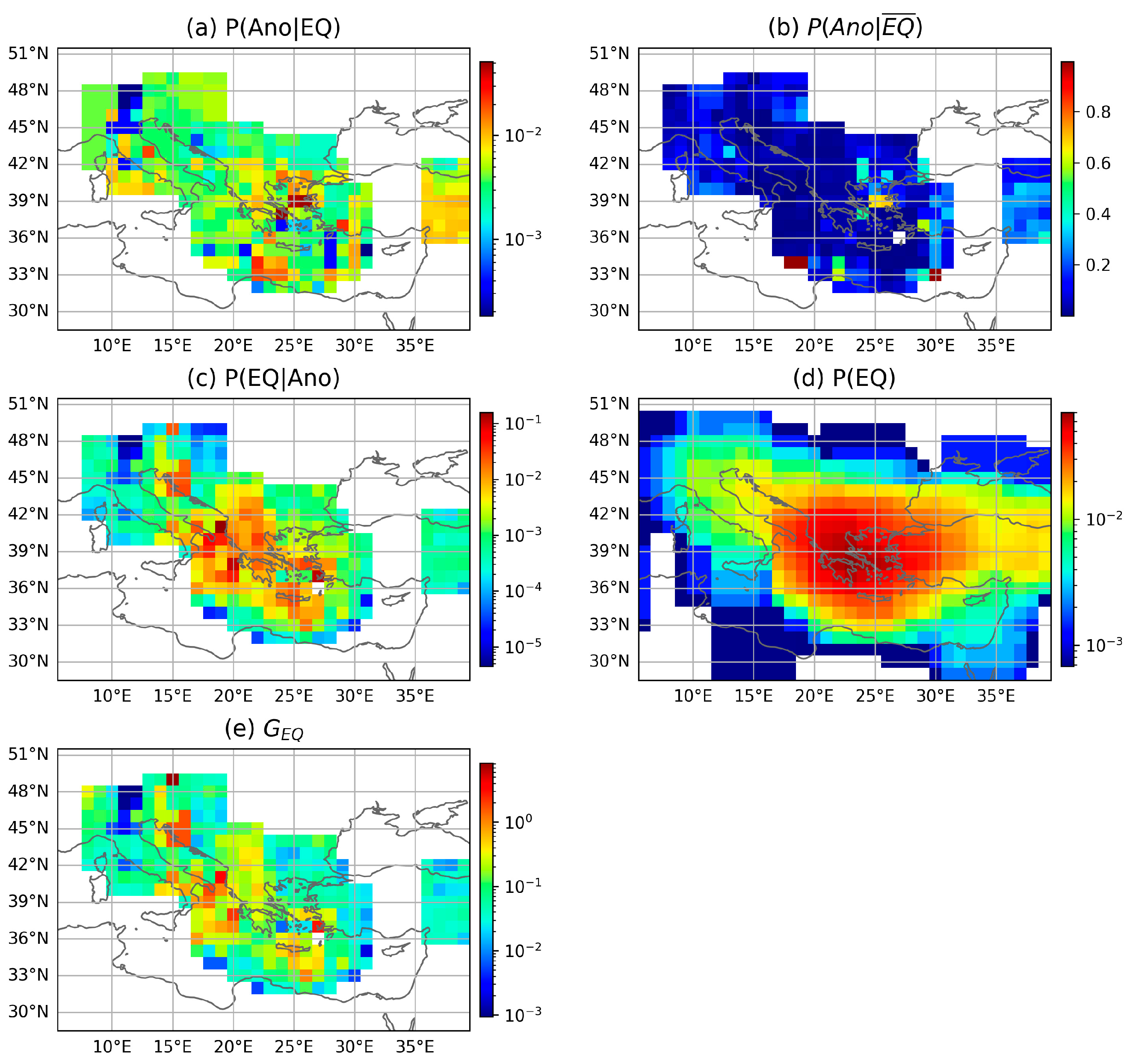
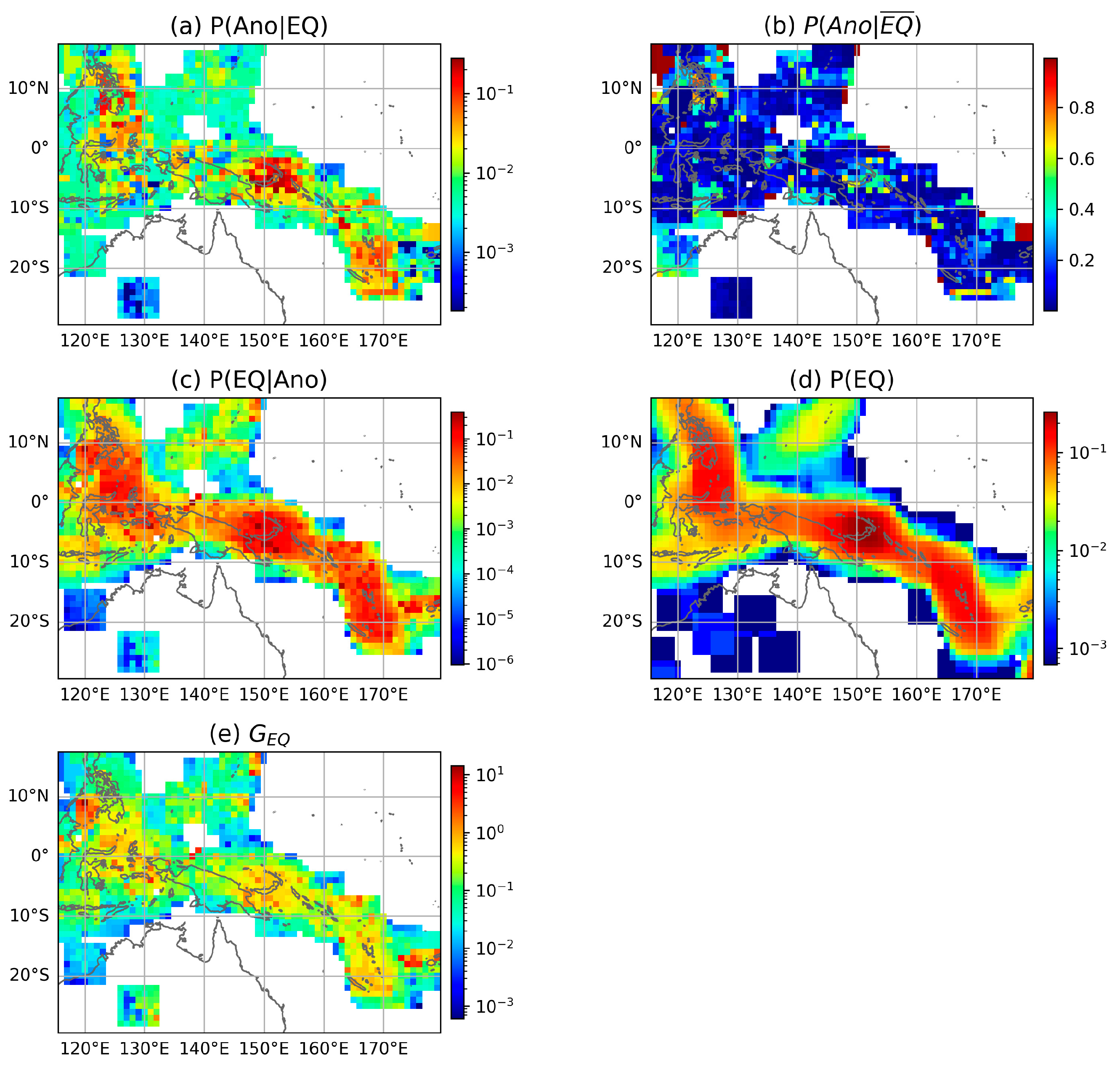
To further illuminate the spatial variability of calculated probabilities in Figure 3, we focus on three seismically active regions: Mainland China and its vicinity (Figure 4), the Mediterranean (Figure 5), and Southeast Asia (Figure 6). As expected, $P\left(Ano|EQ\right)$ consistently exceeds $P\left(Ano|\overline{EQ}\right)$ in Figure 4a,b, corroborating our previous findings of a higher false-alarm ratio in the study area [31]. However, $P\left(EQ|Ano\right)$ exhibits regional hotspots within the north–south and the Xinjiang Pamir to Tianshan north–south seismic belts (Figure 4c). Especially, the Taiwan region emerges as a hotspot with $P\left(EQ\right)$ values surpassing 0.15 (Figure 4d). Figure 4e reveals several regions within the high-probability areas of Figure 4c where $G_{EQ}$ exceeds 1. This signifies that OLR anomalies in these regions effectively enhance the forecast capacity for imminent strong earthquakes. Similar patterns emerge in the Mediterranean, where OLR anomalies can offer $P\left(EQ|Ano\right)$ values exceeding 0.05, considering a maximum $P\left(EQ\right)$ of 0.08 (Figure 5). In Southeast Asia, Figure 6d presents higher $P\left(EQ\right)$ values, reaching up to 0.25, and Figure 6e highlights extensive areas with $G_{EQ}$ greater than 1. This suggests that OLR anomalies can meaningfully contribute to earthquake forecasts within these regions, particularly in Indonesia and the Philippines.

Overall, these findings demonstrate a significant benefit in utilizing OLR anomalies for earthquake forecasts. While a phenomenological occurrence alone does not constitute definitive proof of precursory behavior, the observed spatial correlation between $P_{EQ}$ and seismically active regions, coupled with the high $G_{EQ}$ values in specific areas, provides compelling evidence supporting the feasibility and potential of a thermal anomaly for global earthquake forecasts.

4.2. Probability Gains of Each Parameter

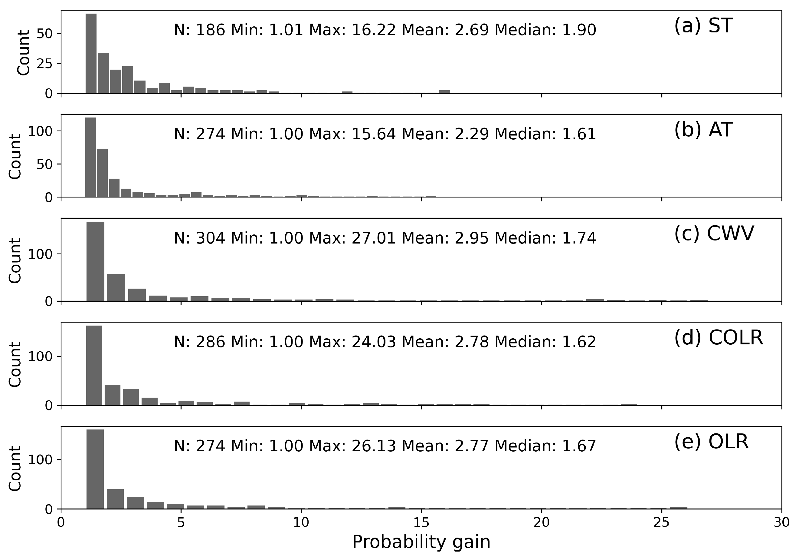
A valid earthquake forecast hypothesis identifies spatiotemporal sub-volumes with statistically elevated probability of strong earthquakes, demonstrably exceeding baseline levels. A valid hypothesis, in the context of earthquake forecasts, exhibits $G_{EQ}$ values consistently exceeding 1. Figure 7 presents the histograms of each parameter for the entirety of the seismically active regions. The statistical distributions exhibit remarkable similarity across all parameters. This uniformity implies that each parameter holds promise for generating valid forecasts within specific regions, notwithstanding the spatial disparities evident in the distribution of $G_{EQ}$ as illustrated in Figure 3 and Figure S1–S4. Consequently, the collective utilization of these parameters possesses the potential to enhance forecasting efficacy across diverse geographical contexts.

In particular, the CWV anomaly has the best performance, albeit with a marginal advantage, with a record of 304 valid pixels, a maximum $G_{EQ}$ of 27.01, and a mean $G_{EQ}$ of 2.95. This could be explained by the hypothesis that water vapor condensation plays a crucial role in generating atmospheric thermal anomalies [35], with anomalous CWV fluctuations potentially reflecting this intermediary process. According to the LAIC model [36], the atmospheric cascade of changes initiates with fluctuations in radon gas concentration. Radon and its progeny particles ionize the surrounding air, producing both positively and negatively charged ions. Subsequent chemical interactions between these newly formed ions and atmospheric water vapor lead to the formation of large hydrated ions, consequently altering relative humidity. In contrast, the AT anomaly exhibits the lowest $G_{EQ}$ of 2.29, with such values indicating a modest risk of large earthquakes [37].

Figure 6. Component analysis of earthquake forecast probability for OLR anomaly on 31 December 2020, focused on Southeast Asia. (a) Probability of OLR anomaly occurrence before earthquakes; (b) probability of OLR anomaly occurrence without earthquakes; (c) posterior probability of earthquake occurrence given the OLR anomaly; (d) natural probability of earthquake occurrence; (e) probability gain from OLR anomaly. See Supplementary Figures S13–S16 for complete analyses of ST, AT, CWV, and COLR anomalies. Data were log10-transformed to emphasize very low values, except for panel (b).

Figure 6. Component analysis of earthquake forecast probability for OLR anomaly on 31 December 2020, focused on Southeast Asia. (a) Probability of OLR anomaly occurrence before earthquakes; (b) probability of OLR anomaly occurrence without earthquakes; (c) posterior probability of earthquake occurrence given the OLR anomaly; (d) natural probability of earthquake occurrence; (e) probability gain from OLR anomaly. See Supplementary Figures S13–S16 for complete analyses of ST, AT, CWV, and COLR anomalies. Data were log10-transformed to emphasize very low values, except for panel (b).

These observations collectively demonstrate the potential of thermal anomalies in earthquake forecasts, irrespective of the specific parameter. Each geophysical parameter exhibits the capability to surpass a $G_{EQ}$ value of 1 in certain regions of heightened seismic activity, thus holding promise for achieving OEF in these areas with credible forecast probabilities. Importantly, the results highlight that while every parameter can contribute precursory information about upcoming earthquakes, no single parameter emerges as definitively superior. The multiparametric approach has caught significant attention, e.g., [6,38], as it is anticipated to enhance earthquake forecasting by assembling a broader spectrum of information pertaining to seismogenic processes. This study underscores the potential value of a multiparametric approach for earthquake forecasts in a quantitatively rigorous manner, combining non-seismological (e.g., land and atmospheric parameters used in this study) and seismological parameters [39].

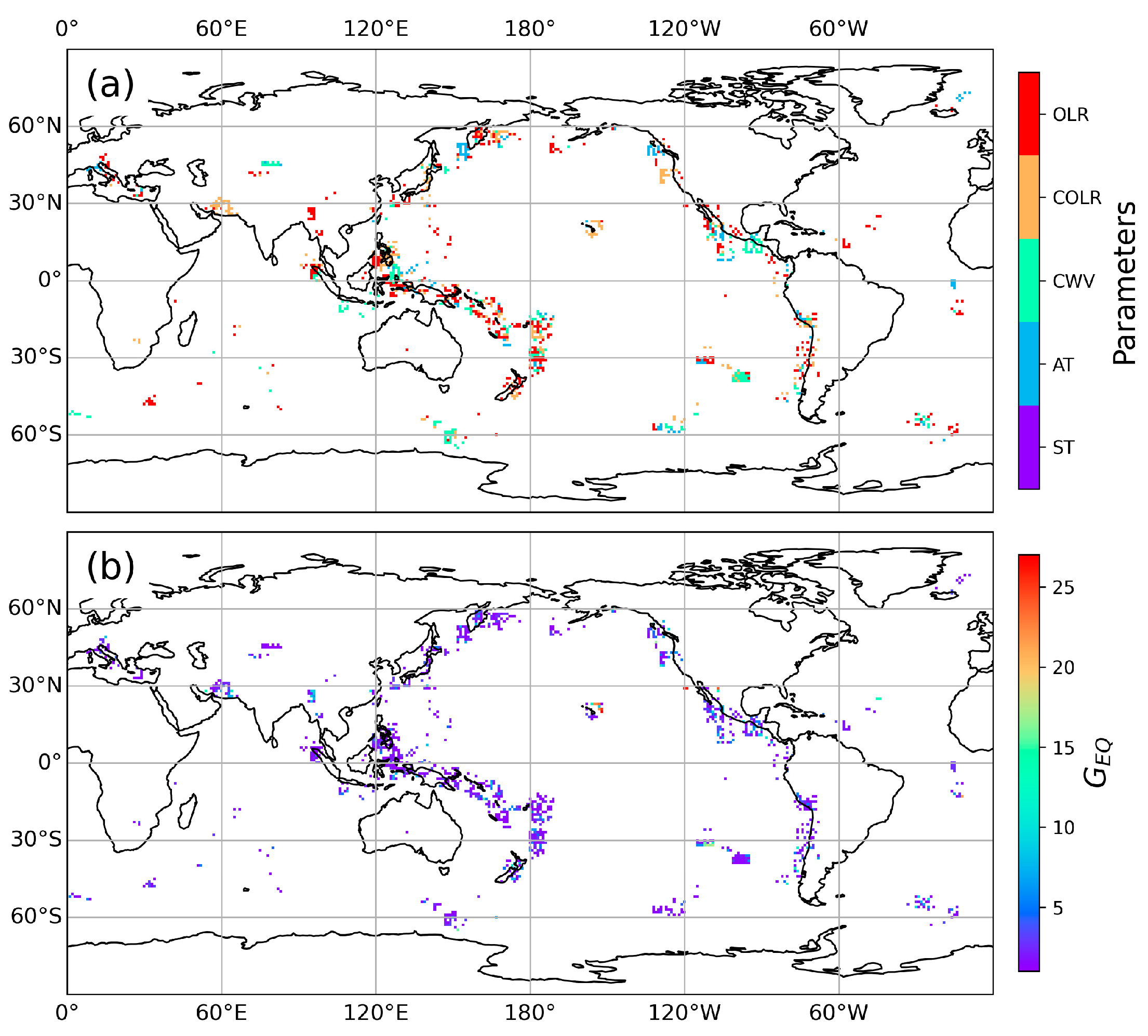
To identify the most informative geophysical parameter for the public communication of earthquake forecasts, we leverage $G_{EQ}$ as a key indicator. A higher $G_{EQ}$ indicates a heightened probability of imminent earthquakes following the observed anomaly. We use $G_{EQ}$ to determine the optimal parameter for each pixel within seismically active regions (Figure 8a). CWV and COLR anomalies occupy larger areas (268 and 251 pixels, respectively), suggesting their potential efficacy in specific zones, while ST, AT, and OLR exhibit lower pixel counts that are 160, 240, and 239, respectively. However, no single parameter demonstrates a clear and consistent advantage across most areas. It should be noted that CWV anomalies are also the best performance shown in Figure 7. Further insights emerge from Figure 8b, where most optimal $G_{EQ}$ values fall below 5, with only 3.2% of areas exceeding 10. $G_{EQ}$ can serve as an additional metric for evaluating earthquake forecast capacity [17]. Ideally, larger areas with high $G_{EQ}$ values (>5–10) should be observed for the most valuable precursor parameters [2]. These results highlight the value of $G_{EQ}$ as a communication tool, while the results also highlight the need for further research to identify parameters with consistently high $G_{EQ}$ over extensive regions.

Figure 7. Histograms of probability gains >1 for AIRS multiparametric anomalies on 31 December 2020.

Figure 7. Histograms of probability gains >1 for AIRS multiparametric anomalies on 31 December 2020.

Figure 8. Optimal combination of five geophysical parameters (i.e., skin temperature, air temperature, total integrated column water vapor burden, outgoing longwave radiation (OLR), and clear-sky OLR) for maximizing earthquake forecast probability. (a) Spatial distribution of each parameter included in optimal combination. (b) Probability gain achieved using optimal parameter combination.

Figure 8. Optimal combination of five geophysical parameters (i.e., skin temperature, air temperature, total integrated column water vapor burden, outgoing longwave radiation (OLR), and clear-sky OLR) for maximizing earthquake forecast probability. (a) Spatial distribution of each parameter included in optimal combination. (b) Probability gain achieved using optimal parameter combination.

4.3. Time Scales for Obtaining the Stable Forecast Probability

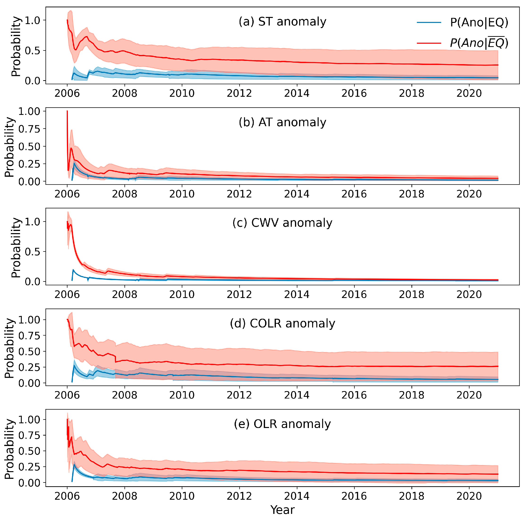
To generate robust estimates of $P_{EQ}$ using five geophysical parameters from the earthquake catalog and AIRS remote sensing product, sufficient data samples are crucial for accurate Bayesian updating calculations. Figure 9 presents a time series from the Taiwan region, exhibiting the number of years required for $P_{EQ}$ to stabilize. Two probability types, i.e., $P\left(Ano|EQ\right)$ and $P\left(Ano|\overline{EQ}\right)$, for each parameter gradually stabilize after 2012, indicating a period of approximately 6 years. While ST and COLR anomalies exhibit greater variations than AT and CWV, $P\left(Ano|EQ\right)$ values remain consistently lower and spatially less variable in the Taiwan region. Figure 10 further details the estimated $P_{EQ}$ values for each parameter within the Taiwan area. AT anomalies contribute the highest $P_{EQ}$, while ST and COLR exhibit the lowest performance across the time series. It highlights the distinct regional characteristics of different TIR parameters in earthquake forecasting. Specifically, within the Taiwan region, AT, COLR, and CWV are preferred for seismic monitoring due to their elevated $P_{EQ}$ values. These $P_{EQ}$ values represent long-term averages, robustly indicating the forecast capacity of each parameter. A higher $P_{EQ}$ stands for an increased likelihood of successfully forecasting impending strong earthquakes in this region. Similar to Figure 9, estimated $P_{EQ}$ values trend towards stability starting around 2012. Collectively, these findings suggest that a minimum of 6 years is a reasonable threshold for obtaining robust estimates of $P_{EQ}$.

4.4. Prospective Analysis of Earthquakes in 2021 and 2022

As Console [10] emphasizes, the ultimate validation of any earthquake forecast hypothesis lies in its independent evaluation against a new set of observations. Accordingly, we apply our proposed method to data from 2021 and 2022, entirely separate from the data used to estimate global $P_{EQ}$ in the previous section. $P_{EQ}$ serves a dual purpose: demonstrating the usability of our scheme for decision making in real-world forecasting scenarios and facilitating the quantitative integration of thermal anomalies with other parameters in earthquake forecast practice. While the implementation of such integrated forecasts falls outside the scope of this study, we showcase the feasibility and applicability of our probability estimation scheme within the context of anomaly recognition.

To this end, we construct two novel anomaly indices incorporating $P_{EQ}$. The first, ${PI}_1$, is defined as the probability of an anomaly occurring at a specific location, given the observed anomaly:

$${PI}_1=P\left(EQ|Ano\right)·Ano,$$

(4)

where Ano denotes the binary anomaly state derived using the approach described in Section 3.1. While ${PI}_1$ can vary across the spatial domain, a specific location will always have a fixed forecast probability. Recognizing this limitation, we introduce a second index, ${PI}_2$, incorporating the calculated anomaly value:

$${PI}_2=P\left(EQ|Ano\right)·Ano·V_{ano},$$

(5)

where $V_{ano}$ is the anomaly value obtained from Equation (1). Thus, ${PI}_2$ can vary spatiotemporally.

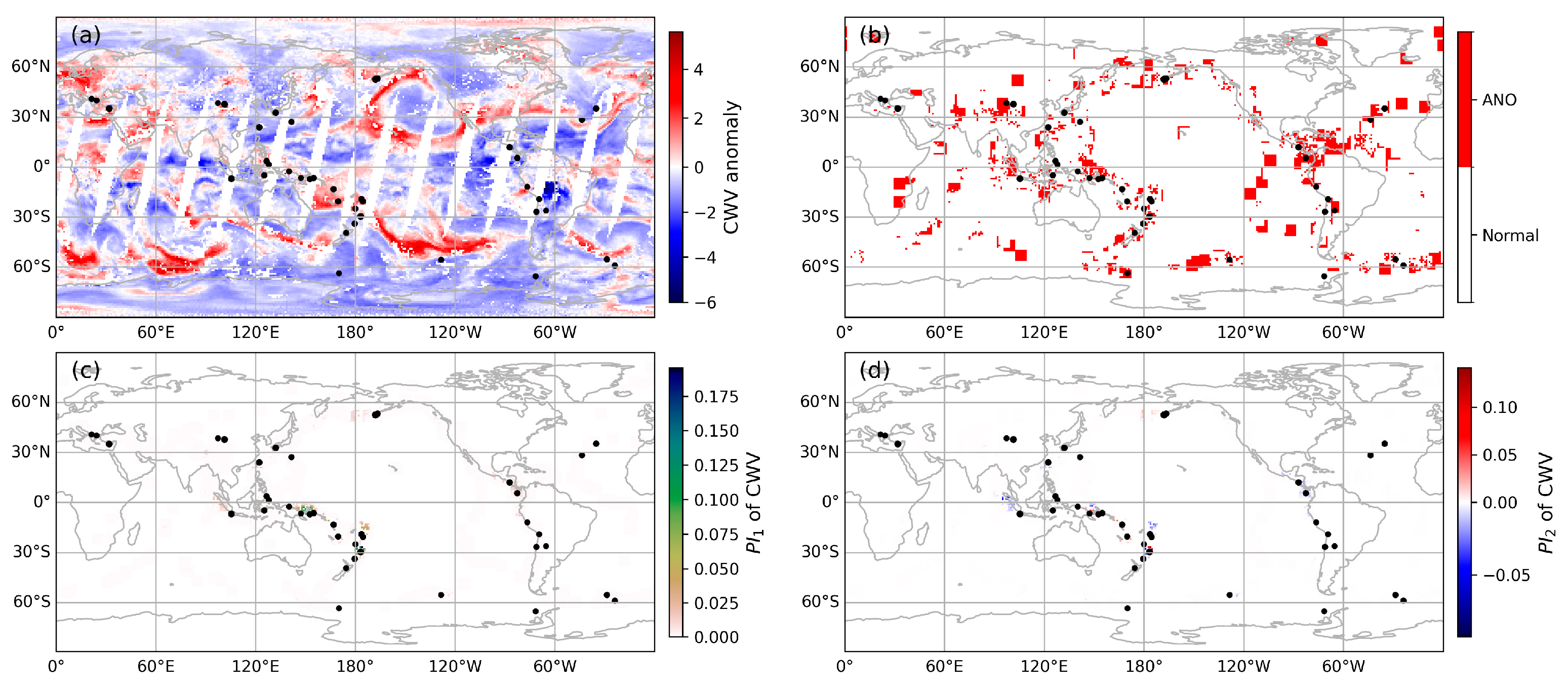
The anomalies computed using Equation (1) are depicted in Figure 11a. Notably, extensive positive and negative anomalies (>3 or <−3) are evident across a vast geographical expanse on a global scale, whereas earthquake occurrences, denoted by black dots, remain sparse. This suggests an issue for significant false alarms across most regions in terms of earthquake forecasts. Therefore, the optimal anomaly recognition criteria were proposed [14], markedly constraining the areas identified as anomalies (Figure 11b). Red zones within these reduced areas denote potential locations for strong earthquakes (black dots), and the possible seismogenic regions have been substantially reduced. Moreover, owing to the incorporation of prior knowledge within these criteria, the red zones consistently align with earthquake-prone regions, thereby enhancing the accuracy of earthquake forecasts. As presented in Figure 11c,d, $P_{EQ}$ can further refine the spatial distribution of anomalies into smaller regions with varying magnitudes of anomalies, as described in Equations (4) and (5). A detailed illustrative example is provided in Figure 12, offering a temporal perspective. Notably, a strong spatial correlation exists between identified anomalies and earthquakes exceeding magnitude 5.5, based on the a priori knowledge from calculated probability to constrain anomalous fluctuations. Significantly fewer regions have valid ${PI}_1$ and ${PI}_2$ values, and they overlay or are close to upcoming strong earthquakes. This promising spatial correlation suggests the potential for improved earthquake forecast accuracy through reduced false-alarm rates.

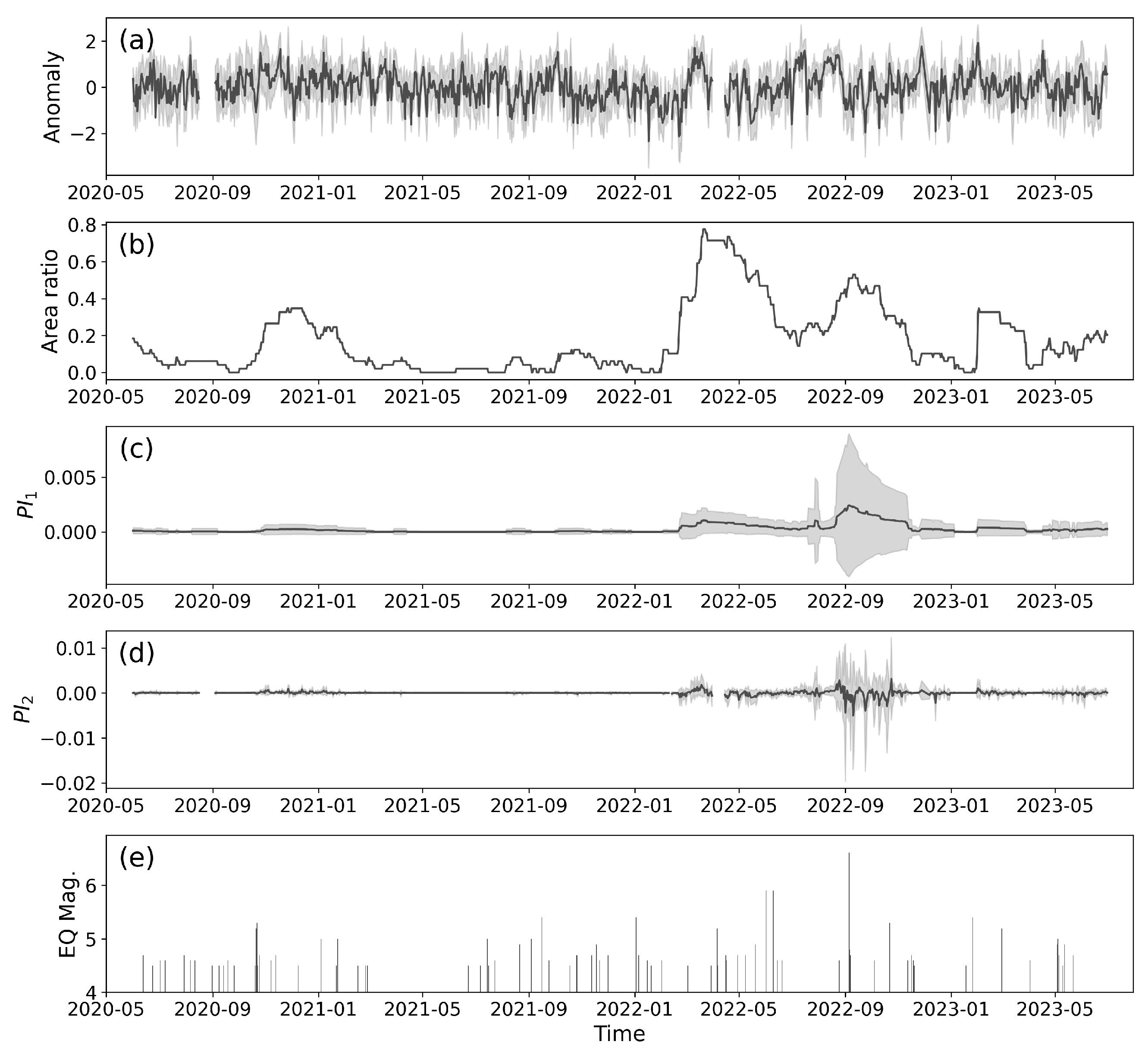
The availability of $P_{EQ}$ is further assessed through the time series of earthquakes exceeding magnitude 5.5 in Mainland China during 2021 and 2022 (

Table 1. Summary of earthquakes with magnitude ≥ 5.5 within Mainland China (70°–110°E, 20°–50°N) in 2021 and 2022. The magnitude (Mag.) type is Mw, except for EQ17 of Mb.

ID	Time (UTC)	Latitude (°)	Longitude (°)	Depth (km)	Mag.
EQ01	19 Mar. 2021 06:11:27.113	31.9244	92.9147	8	5.7
EQ02	28 Apr. 2021 02:21:26.221	26.7819	92.4586	34	6
EQ03	21 May 2021 18:04:13.557	34.5884	98.2402	10	7.3
EQ04	21 May 2021 13:48:37.268	25.7444	100.0155	9	6.1
EQ05	10 Jul. 2021 02:14:43.154	38.9169	70.5539	12.84	5.7
EQ06	25 Nov. 2021 23:45:41.780	22.8217	93.52	42.72	6.2
EQ07	24 Dec. 2021 13:43:22.983	22.3639	101.6878	10	5.7
EQ08	7 Jan. 2022 17:45:30.751	37.8152	101.2775	13	6.6
EQ09	23 Jan. 2022 02:21:19.926	38.4613	97.3425	10	5.6
EQ10	25 Mar. 2022 16:21:04.052	38.5196	97.2683	10	5.7
EQ11	1 Jun. 2022 09:00:08.122	30.4155	102.9892	10	5.9
EQ12	9 Jun. 2022 17:28:37.438	32.3747	101.9033	14.37	5.9
EQ13	9 Jun. 2022 16:03:26.522	32.3152	101.8363	10.14	5.6
EQ14	21 Jul. 2022 17:07:25.214	21.155	99.8813	5	5.9
EQ15	5 Sep. 2022 04:52:19.634	29.6856	102.2278	12	6.6
EQ16	8 Nov. 2022 20:27:23.418	29.2742	81.1486	18.082	5.7
EQ17	28 Dec. 2022 17:16:36.243	41.8052	79.5408	10	5.6

). We illustrate an example case in Figure 12. The comparison of the time series of ST anomalies (Figure 12a) and earthquakes with magnitude > 4.5 (Figure 12e) reveals insufficient information to reliably identify pre-seismic anomalies due to the continuous and irregular fluctuations of ST anomalies throughout the analysis period. However, the area ratio of identified anomalies exhibits several peaks in November 2021, March and October 2022, and February 2023 (Figure 12b), suggesting that anomalies occurred in a larger number of areas within a 7 × 7 window during these periods. Notably, the maximum peak value precedes the occurrence of EQ15 listed in Table 1. Figure 12c demonstrates that more significant anomalous fluctuations commence on 3 February 2022, and reach their peak on 5 September 2022, coinciding with the date of the major earthquake (EQ15). The disturbance then gradually attenuates, accompanied by aftershocks. The variations of ${PI}_2$ exhibit similar characteristics to those of ${PI}_1$, and the anomalous values induce ${PI}_2$ to generate numerous significant pulses surrounding the time of EQ15, indicating a substantial spatial perturbation of ST anomalies. These findings highlight the valuable role of the new anomaly indices in effective anomaly detection.

Despite Figure 12 showcasing an encouraging example, the $P_{EQ}$ itself implicitly acknowledges the absence of consistent pre-seismic correlation across all seismic events, considering its very low values. Additional insights are revealed in

Table 2. Performance of anomaly indices in identifying earthquakes from Table 1. The values 1 and 0 denote valid and invalid anomalies prior to earthquakes, respectively.

ID	ST	AT	CWV	COLR	OLR	Count
EQ01	1	1	0	1	1	4
EQ02	0	1	0	1	0	2
EQ03	0	1	1	1	1	4
EQ04	0	0	1	0	1	2
EQ05	1	0	1	1	1	4
EQ06	0	1	0	0	0	1
EQ07	0	0	1	0	0	1
EQ08	0	1	1	0	0	2
EQ09	0	0	1	0	0	1
EQ10	0	0	1	0	0	1
EQ11	1	1	0	1	1	4
EQ12	1	1	0	1	1	4
EQ13	1	1	0	0	0	2
EQ14	1	1	0	0	0	2
EQ15	1	1	0	1	0	3
EQ16	0	0	1	1	0	2
EQ17	0	1	1	0	0	2
Count	7	11	9	8	6	41

, which highlights three key observations. (1) Every earthquake exhibits some level of anomalous behavior across various geophysical parameters. (2) Most earthquakes feature anomalies in at least two different parameters, as exemplified by the AT and COLR anomalies preceding EQ2. (3) Remarkably, no single parameter consistently dominates within the listed earthquakes, with valid anomaly counts ranging from 6 to 11 (35.3% to 64.7% of total events). These observations could be linked with the Lithosphere–Atmosphere–Ionosphere Coupling (LAIC) model, which posits the interaction and energy transfer between diverse anomalous phenomena within the lithosphere, atmosphere, ionosphere, and magnetosphere during the precursory stages of long-term seismic activity [35,40]. The LAIC model expects and explains the observed lack of a single dominant parameter, emphasizing the potential presence of statistically significant spatiotemporal correlations across multiple parameters preceding major earthquakes theoretically [38].

4.5. A Probabilistic Synthesis of Anomalies for Five Geophysical Parameters

Considering the limitations of individual parameters, a multiparametric approach emerges as a promising avenue for enhancing earthquake probability estimation. To test the effectiveness of ensemble forecasts, we implement the capped eigenvalue (CE) method, which harnesses the strengths of multiple models and/or earthquake precursors through a weighted mean [41]. While the CE method satisfies desirable properties like dilution and monotonicity, it falls short of the strong dilution property, leading to weight adjustment when adding an identical model. Marzocchi, et al. [25] deems such adjustment as often negligible, even if theoretically undesirable. To quantify the interdependence between anomaly forecasts, the concept of forecast correlation is introduced, defined as a correlation matrix derived from Pearson’s correlation coefficients:

$$C=\left[\begin{array}{cccc}{c}_{11}& c_{12}& \cdots & c_{1N}\\ c_{21}& c_{22}& \dots & c_{2N}\\ \dots & \dots & \dots & \dots \\ c_{N1}& c_{N2}& \dots & c_{NN}\end{array}\right],$$

(6)

where N is the number of anomaly parameters and c represents the Pearson’s correlation coefficients between two types of $P_{EQ}$ (e.g., ST and AT). Applying this calculation to all valid pixel data within seismically active regions, we obtain the correlation matrix C presented in

Table 3. Correlation matrix and weights of earthquake forecast probabilities for anomalies derived from five studied geophysical parameters: skin temperature (ST), air temperature (AT), total integrated column water vapor burden (CWV), outgoing longwave radiation (OLR), and clear-sky OLR (COLR). The hyphen denotes the concealment of the repetitive values in the upper triangular matrix.

	ST	AT	CWV	COLR	OLR
ST	1.000	0.360	0.415	0.385	0.354
AT	-	1.000	0.326	0.369	0.372
CWV	-	-	1.000	0.387	0.349
COLR	-	-	-	1.000	0.363
OLR	-	-	-	-	1.000
Weight	0.196	0.204	0.200	0.197	0.203

. The correlation coefficients between $P_{EQ}$ values of different parameters consistently range from 0.3 to 0.4, with the highest value reaching 0.415 between $P_{EQ}$ values for ST and CWV anomalies. This moderate correlation persists despite the observed spatial variations in individual anomaly patterns, as illustrated in Figure 3 and Figure S1–S4.

To account for the observed forecast correlation, the CE scheme leverages the spectral decomposition of the correlation matrix C as described by Garthwaite and Mubwandarikwa [41]:

$$C=Q\Lambda Q^T,$$

(7)

where $\Lambda$ is the diagonal eigenvalue matrix, Q contains the normalized eigenvectors in its columns, and $Q^T$ is the transpose of Q. Any eigenvalue >1 signifies redundant information within the model, as the maximum value for each element of C is 1. The CE method addresses this redundancy by transforming $\mathrm{\Lambda }$ to ${\mathrm{\Lambda }}^{\mathrm{*}}$ through eigenvalue capping: any element in $\mathrm{\Lambda }$ exceeding 1 is set to 1, while all others remain unchanged. Then, the diagonal elements of $C^{\mathrm{*}}=Q{\mathrm{\Lambda }}^{\mathrm{*}}{Q}^T$ are normalized to sum to one and serve as the weights presented in Table 3. These weights cluster around 0.2, suggesting an approximately equal contribution from each of the five anomaly parameters. This observation reinforces the earlier conclusion that, within our analyzed parameters, no single geophysical parameter exhibits a clear advantage in predicting future strong earthquakes. The final ensemble probability ($\widehat{P}$) is then calculated by multiplying these weights:

$$\widehat{P}=\frac{{\sum }_{i=1}^N{C}_{ii}^{*}·P_i\left(EQ|ANO\right)}{{\sum }_{i=1}^N{C}_{ii}^{*}},$$

(8)

where $C_{ii}^{\mathrm{*}}$ is the ith element in $C^{\mathrm{*}}$.

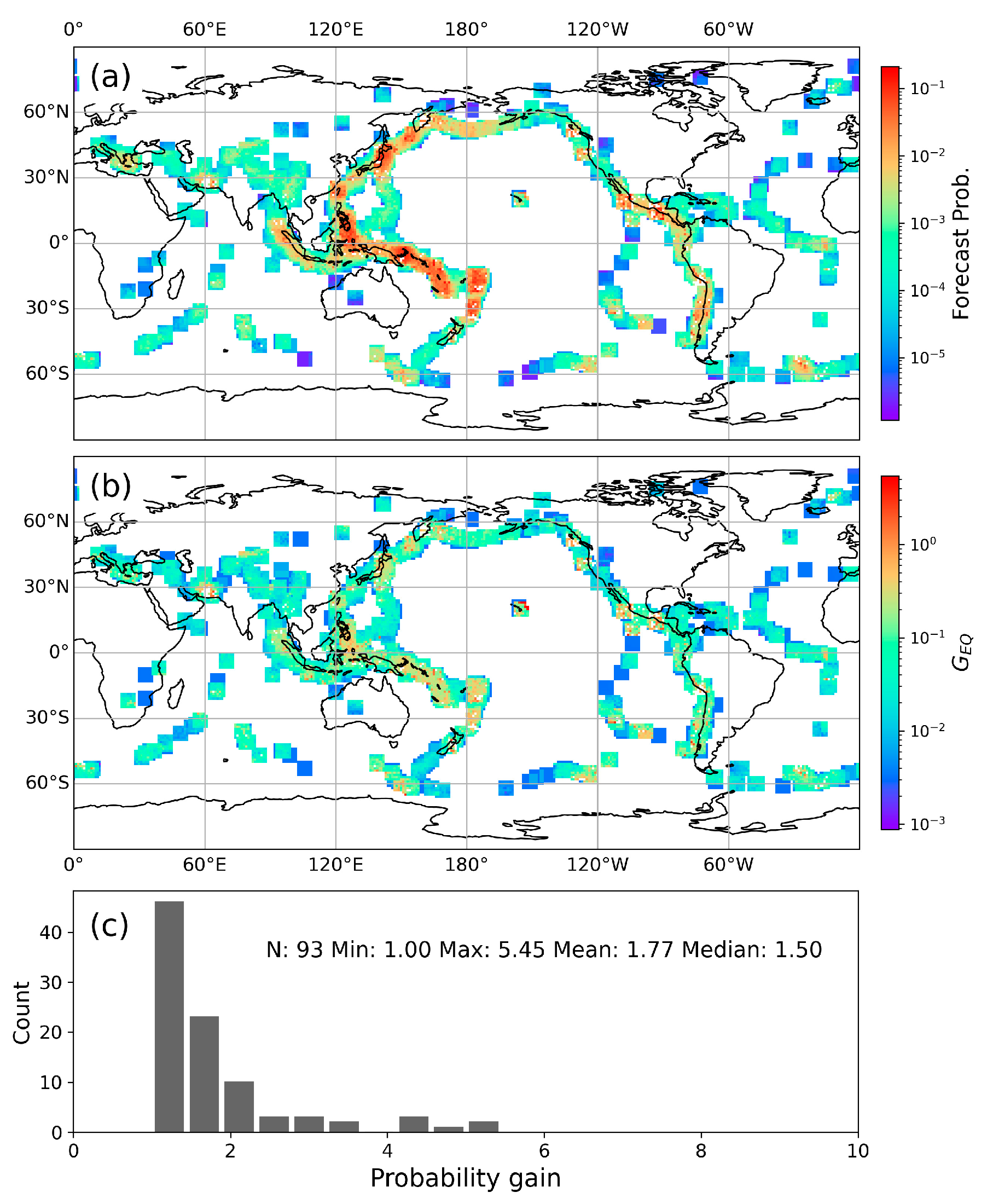
Figure 13 presents the final ensemble forecast probability map. It closely resembles the average of global $P_{EQ}$ maps derived from each individual parameter (cf. Section 4.1), suggesting a near-neutral influence of the CE method on the spatial distribution of the ensemble forecast. However, closer examination reveals $G_{EQ}$ performance degradation compared to individual parameters. This decline is evident in the reduced number of valid pixels (93) and the lower mean $G_{EQ}$ value (1.77) of the ensemble forecast, as shown in Figure 13c and contrasted with Figure 7. These observations raise concerns about the general effectiveness of the CE method advised by Marzocchi, et al. [25] for achieving optimal performance in terms of $G_{EQ}$. Further research is warranted to explore alternative ensemble strategies that can effectively combine information from diverse thermal anomalies, potentially even across distinct disciplines [5], to unlock the full potential of multiparametric earthquake forecasts.

5. Discussion

Historically, OEF methods have been hampered by significant limitations in both the accuracy of their estimated probabilities that are often unrealistically low, and their general applicability that is biased towards earthquakes with foreshocks [42]. In contrast, our approach, drawing on the Bayesian formula and historical data, enables the direct calculation of the $P_{EQ}$ without additional assumptions, representing a potential advancement over existing methods [23,33], which, for instance, rely on factors such as earthquake clustering, potential foreshock sequences, the relation between covariance and cross-correlation, or fault geometry models. Significantly, our method can be universally applied across seismically active regions, extending beyond specific experimental areas such as southern California [33], and in certain earthquake-prone regions, yields $P_{EQ}$ values better than 0.1. Typically, probabilities of an earthquake occurrence range from negligibly small values (e.g., 0.001%) to larger magnitudes (e.g., 5%) [42,43]. Importantly, the application of new anomaly indices reduces the influence of anomalous fluctuations unrelated to the seismic preparation phase, despite not explicitly addressing the underlying cause–effect mechanisms. These results pave the way for more effective pre-seismic anomaly recognition and demonstrate the potential feasibility of earthquake forecasts based on thermal anomalies.

Our map of static global $P_{EQ}$ based on anomalies of five geophysical parameters demonstrates remarkable stability after roughly six years (cf. Section 4.3). This stability reflects the long-term average influence of each parameter on earthquake probability estimation. The $P_{EQ}$ map serves as a valuable guide for evaluating upcoming earthquakes based on identified anomalies and quantitatively integrating those assessments with other anomalous information from factors such as geomagnetic and seismological observations [5], as well as ionospheric total electron content [44,45]. While operational earthquake monitoring and forecasts remain a significant challenge, the crucial step for effective OEF systems lies in estimating the dynamic $P_{EQ}$ map, capturing the short-term responses to impending earthquakes. Future research will focus on developing such a time-dependent earthquake forecast model founded upon sequential Bayesian inference, with explicit modeling of probability distribution functions for model parameters. This approach will leverage satellite data and potentially integrate fault information, wherein estimated earthquake rupture probabilities of fault segments can serve as background information for earthquake forecasts, employing newly updated thermal anomaly data [34,46].

Our findings underscore the absence of a single dominant precursory parameter, therefore highlighting the need for further research focused on improving both anomaly detection methods and recognition criteria. While the ZS method proves to be suitable for this study, a comprehensive and quantitative evaluation of additional approaches is crucial to identify potentially superior techniques. Our compiled list of anomaly detection methods, characterized by their relative simplicity and broad applicability [4], provides a robust starting point for such a comparative analysis. For instance, the Robust Satellite Technique (RST) anomaly detection method, considered a variant of the ZS method, introduces neighbor differences to emphasize spatial variations while maintaining a straightforward mathematical formulation. It has been extensively used across various seismic events and satellite data sources [47,48,49,50], which represents significant progress in identifying pre-earthquake anomalous phenomena. As Console [10] observed, systematic testing of the numerous, often proponent-driven, earthquake prediction methodologies has been hampered by the lack of both a rigorous quantitative definition of precursory signals and continuous, high-quality observational data. By implementing a quantitative comparison framework like the one presented here, we can effectively filter out approaches that fail to reliably capture anomalous characteristics, thus paving the way for their integration into OEF systems. Furthermore, the recent success of deep learning techniques in diverse fields, including earthquake anomaly detection [51], raises promising possibilities for their application to thermal anomalies in future research.

While a statistical correlation between pre-seismic anomalies and earthquakes suggests a potential connection, it does not imply direct causation. For instance, the pre-existing coincidence of high background heat flow and seismicity [52] can be one of the factors influencing the correlation between thermal anomalies and seismicity. While they are not entirely independent, differentiating thermo-seismic events is beneficial for thermal-based earthquake forecasts. A co-kriging approach to separate seismic and thermal signals appears to be promising, thus mitigating potential adverse effects. Meanwhile, several physical mechanisms have been proposed to explain the underlying link between thermal anomalies and seismic events [4,53]. Firstly, the earth degassing theory [54] posits that microcrack initiation and the release of greenhouse gases such as CO₂ and CH₄ into the lower atmosphere occur under strengthened stress conditions around the seismogenic region. Changes in convective heat flux, manifested as hot water and gas, alter the earth’s surface temperature. Moreover, greenhouse gases absorb a portion of the earth’s infrared radiation, leading to the accumulation of heat near the surface. Secondly, the temperature–stress theory [55,56,57] suggests that during the loading process, stress transfer—due to the elastic deformation of rock—can be accompanied with the increment of TIR radiation. Following rock failure, TIR temperatures decrease as vertical stress diminishes. Thirdly, the p-hole activation theory [58,59] demonstrates that electronic charge carriers are released when peroxy links break in stressed rocks, and reach the earth’s surface, ionizing the air at the ground–air interface. The recombination of charge carriers at the surface results in a spectroscopically distinct, non-TIR emission [58,59]. On top of that, the LAIC model [35,40] has gained considerable traction and offers a plausible framework for interpreting the results of this study. However, the LAIC model itself has multiple, and potentially distinct, driving mechanisms, including radon emission [35], peroxy defects [60], and atmospheric gravity/acoustic wave effects [61]. Additionally, there is the study suggesting a mixed driving mechanism responsible for generating anomalous phenomena within the atmosphere and ionosphere [62].

These hypotheses remain largely rooted in laboratory observations and theoretical conjectures. To solidify and refine these proposed mechanisms, further field experiments and robust physical modeling are essential. The observations indicate that seismically active zones exhibit high thermal radiance [52], and there are discernible temporal thermal anomalies preceding earthquakes. Such field evidence is critical for validating or constraining the hypotheses. While unraveling the physical underpinnings of pre-seismic anomalies constitutes the ultimate goal for achieving physical-based earthquake forecasts, the development of statistics-based forecast methods, as presented in this study, can proceed even without a complete understanding of the underlying mechanisms. The urgency of earthquake preparedness and the growing potential of data-driven deep learning models stress the importance of pursuing both statistical and physical avenues for earthquake forecasts in parallel.

6. Conclusions

This study investigated the potential of pre-seismic thermal anomalies, derived from five satellite-based geophysical parameters, for global earthquake forecasts. We employed an optimally tuned, spatially self-adaptive multiparametric anomaly identification scheme to refine anomalies, and then estimated the posterior probability of earthquake occurrences given observed anomalies within a Bayesian framework.

Our findings offer a promising path for improving earthquake preparedness and OEF systems. Thermal anomalies exhibit a statistically significant spatial correlation with seismically active regions, with elevated forecasting probabilities better than 0.1 observed in areas prone to strong events. While no single parameter consistently dominates, each contributes precursory information, suggesting an encouraging avenue for a multi-parametric approach. Furthermore, a minimum of six years of observed data is crucial for robust probability estimation. Applying the estimated probabilities to data from 2021 to 2022 strengthens the practical potential of the model, showcasing promising correlations between identified anomalies and earthquakes. However, challenges remain, including exploring alternative ensemble strategies and establishing comprehensive validation protocols for anomaly detection methods.

This study provides compelling evidence for the potential of pre-seismic thermal anomalies as valuable indicators for global earthquake forecasts. With continued research and collaboration, thermal anomalies can play a vital role in mitigating earthquake risk and saving lives. By addressing the identified challenges and pursuing both statistical and physical paths in parallel, we can accelerate the development of robust and reliable OEF systems, ultimately making the world a safer place.

References

1. Rundle, J.B.; Stein, S.; Donnellan, A.; Turcotte, D.L.; Klein, W.; Saylor, C. The complex dynamics of earthquake fault systems: New approaches to forecasting and nowcasting of earthquakes. Rep. Prog. Phys. 2021, 84, 076801. [Google Scholar] [CrossRef] [PubMed]
2. Sykes, L.R. Intermediate- and long-term earthquake prediction. Proc. Natl. Acad. Sci. USA 1996, 93, 3732. [Google Scholar] [CrossRef] [PubMed]
3. Falcone, G.; Spassiani, I.; Ashkenazy, Y.; Shapira, A.; Hofstetter, R.; Havlin, S.; Marzocchi, W. An Operational Earthquake Forecasting Experiment for Israel: Preliminary Results. Front. Earth Sci. 2021, 9, 729282. [Google Scholar] [CrossRef]
4. Jiao, Z.-H.; Zhao, J.; Shan, X. Pre-seismic anomalies from optical satellite observations: A review. Nat. Hazards Earth Syst. Sci. 2018, 18, 1013–1036. [Google Scholar] [CrossRef]
5. De Santis, A.; De Franceschi, G.; Spogli, L.; Perrone, L.; Alfonsi, L.; Qamili, E.; Cianchini, G.; Di Giovambattista, R.; Salvi, S.; Filippi, E.; et al. Geospace perturbations induced by the Earth: The state of the art and future trends. Phys. Chem. Earth Parts A/B/C 2015, 85–86, 17–33. [Google Scholar] [CrossRef]
6. Satti, M.S.; Ehsan, M.; Abbas, A.; Shah, M.; de Oliveira-Júnior, J.F.; Naqvi, N.A. Atmospheric and ionospheric precursors associated with M ≥ 6.5 earthquakes from multiple satellites. J. Atmos. Sol.-Terr. Phys. 2022, 227, 105802. [Google Scholar] [CrossRef]
7. Shah, M.; Ehsan, M.; Abbas, A.; Ahmed, A.; Jamjareegulgarn, P. Possible Thermal Anomalies Associated With Global Terrestrial Earthquakes During 2000–2019 Based on MODIS-LST. IEEE Geosci. Remote Sens. Lett. 2022, 19, 1–5. [Google Scholar] [CrossRef]
8. Salh, H.; Muhammad, A.; Ghafar, M.M.; Külahcı, F. Potential utilization of air temperature, total electron content, and air relative humidity as possible earthquake precursors: A case study of Mexico M7.4 earthquake. J. Atmos. Sol.-Terr. Phys. 2022, 237, 105927. [Google Scholar] [CrossRef]
9. Marchetti, D.; De Santis, A.; Shen, X.; Campuzano, S.A.; Perrone, L.; Piscini, A.; Di Giovambattista, R.; Jin, S.; Ippolito, A.; Cianchini, G.; et al. Possible Lithosphere-Atmosphere-Ionosphere Coupling effects prior to the 2018 Mw = 7.5 Indonesia earthquake from seismic, atmospheric and ionospheric data. J. Asian Earth Sci. 2020, 188, 104097. [Google Scholar] [CrossRef]
10. Console, R. Testing earthquake forecast hypotheses. Tectonophysics 2001, 338, 261–268. [Google Scholar] [CrossRef]
11. Geller, R.J. Earthquake prediction: A critical review. Geophys. J. Int. 1997, 131, 425–450. [Google Scholar] [CrossRef]
12. Chen, H.; Qin, S.; Xue, L.; Yang, B.; Zhang, K. Universal precursor seismicity pattern before locked-segment rupture and evolutionary rule for landmark earthquakes. Geosci. Front. 2022, 13, 101314. [Google Scholar] [CrossRef]
13. Jordan, T.H.; Chen, Y.-T.; Gasparini, P.; Madariaga, R.; Main, I.; Marzocchi, W.; Papadopoulos, G.; Sobolev, G.; Yamaoka, K.; Zschau, J. Operational earthquake forecasting: State of Knowledge and Guidelines for Utilization. Ann. Geophys. 2011, 54, 316–391. [Google Scholar]
14. Jiao, Z.; Hao, Y.; Shan, X. A Spatially Self-Adaptive Multiparametric Anomaly Identification Scheme Based on Global Strong Earthquakes. Remote Sens. 2023, 15, 3803. [Google Scholar] [CrossRef]
15. Fu, C.-C.; Lee, L.-C.; Ouzounov, D.; Jan, J.-C. Earth’s Outgoing Longwave Radiation Variability Prior to M ≥ 6.0 Earthquakes in the Taiwan Area During 2009–2019. Front. Earth Sci. 2020, 8, 364. [Google Scholar] [CrossRef]
16. Pavlidou, E.; van der Meijde, M.; van der Werff, H.; Hecker, C. Time Series Analysis of Land Surface Temperatures in 20 Earthquake Cases Worldwide. Remote Sens. 2018, 11, 61. [Google Scholar] [CrossRef]
17. Fidani, C. West Pacific Earthquake Forecasting Using NOAA Electron Bursts With Independent L-Shells and Ground-Based Magnetic Correlations. Front. Earth Sci. 2021, 9, 673105. [Google Scholar] [CrossRef]
18. Shen, Z.-K.; Jackson, D.D.; Kagan, Y.Y. Implications of Geodetic Strain Rate for Future Earthquakes, with a Five-Year Forecast of M5 Earthquakes in Southern California. Seismol. Res. Lett. 2007, 78, 116–120. [Google Scholar] [CrossRef]
19. Jackson, D.D.; Kagan, Y.Y. Testable Earthquake Forecasts for 1999. Seismol. Res. Lett. 1999, 70, 393–403. [Google Scholar] [CrossRef]
20. Petersen, M.D.; Cao, T.; Campbell, K.W.; Frankel, A.D. Time-independent and Time-dependent Seismic Hazard Assessment for the State of California: Uniform California Earthquake Rupture Forecast Model 1.0. Seismol. Res. Lett. 2007, 78, 99–109. [Google Scholar] [CrossRef]
21. Nayak, K.; Romero-Andrade, R.; Sharma, G.; Zavala, J.L.C.; Urias, C.L.; Trejo Soto, M.E.; Aggarwal, S.P. A combined approach using b-value and ionospheric GPS-TEC for large earthquake precursor detection: A case study for the Colima earthquake of 7.7 Mw, Mexico. Acta Geod. Et Geophys. 2023, 58, 515–538. [Google Scholar] [CrossRef]
22. Field, E.H.; Jordan, T.H.; Page, M.T.; Milner, K.R.; Shaw, B.E.; Dawson, T.E.; Biasi, G.P.; Parsons, T.; Hardebeck, J.L.; Michael, A.J.; et al. A Synoptic View of the Third Uniform California Earthquake Rupture Forecast (UCERF3). Seismol. Res. Lett. 2017, 88, 1259–1267. [Google Scholar] [CrossRef]
23. Fidani, C.; Gherardi, F.; Facca, G.; Pierotti, L. Correlation between small earthquakes and CO2 anomalies in spring waters: A statistical experiment on the probability of seismic occurrence. Front. Earth Sci. 2023, 11, 1128949. [Google Scholar] [CrossRef]
24. Wei, G.; Chen, K.; Meng, H. Bayesian Inversion of Finite-Fault Earthquake Slip Model Using Geodetic Data, Solving for Non-Planar Fault Geometry, Variable Slip, and Data Weighting. J. Geophys. Res. Solid Earth 2023, 128, e2022JB025225. [Google Scholar] [CrossRef]
25. Marzocchi, W.; Zechar, J.D.; Jordan, T.H. Bayesian Forecast Evaluation and Ensemble Earthquake Forecasting. Bull. Seismol. Soc. Am. 2012, 102, 2574–2584. [Google Scholar] [CrossRef]
26. Darzi, A.; Halldorsson, B.; Hrafnkelsson, B.; Vogfjörð, K.S. Short-term Bayesian ETAS spatiotemporal forecasting of the Ölfus 2008 earthquake sequence in Iceland. Tectonophysics 2022, 839, 229522. [Google Scholar] [CrossRef]
27. Dong, E.; Shcherbakov, R.; Goda, K. Testing the forecasting skills of aftershock models using a Bayesian framework. Front. Appl. Math. Stat. 2023, 9, 1126511. [Google Scholar] [CrossRef]
28. Jaumé, S.C.; Sykes, L.R. Evolving Towards a Critical Point: A Review of Accelerating Seismic Moment/Energy Release Prior to Large and Great Earthquakes. In Seismicity Patterns, their Statistical Significance and Physical Meaning; Wyss, M., Shimazaki, K., Ito, A., Eds.; Birkhäuser: Basel, Switzerland, 1999; pp. 279–305. [Google Scholar]
29. Jiao, Z.; Shan, X. Pre-Seismic Temporal Integrated Anomalies from Multiparametric Remote Sensing Data. Remote Sens. 2022, 14, 2343. [Google Scholar] [CrossRef]
30. Jenkins, A.P.; Biggs, J.; Rust, A.C.; Rougier, J.C. Decadal Timescale Correlations Between Global Earthquake Activity and Volcanic Eruption Rates. Geophys. Res. Lett. 2021, 48, e2021GL093550. [Google Scholar] [CrossRef]
31. Jiao, Z.-H.; Shan, X. Statistical framework for the evaluation of earthquake forecasting: A case study based on satellite surface temperature anomalies. J. Asian Earth Sci. 2021, 211, 104710. [Google Scholar] [CrossRef]
32. Chahine, M.T.; Pagano, T.S.; Aumann, H.H.; Atlas, R.; Barnet, C.; Blaisdell, J.; Chen, L.; Divakarla, M.; Fetzer, E.J.; Goldberg, M.; et al. AIRS: Improving weather forecasting and providing new data on greenhouse gases. Bull. Am. Meteorol. Soc 2006, 87, 911–926. [Google Scholar] [CrossRef]
33. Schorlemmer, D.; Gerstenberger, M.C.; Wiemer, S.; Jackson, D.D.; Rhoades, D.A. Earthquake Likelihood Model Testing. Seismol. Res. Lett. 2007, 78, 17–29. [Google Scholar] [CrossRef]
34. Zechar, J.D.; Jordan, T.H. Testing alarm-based earthquake predictions. Geophys. J. Int. 2008, 172, 715–724. [Google Scholar] [CrossRef]
35. Pulinets, S.; Ouzounov, D. Lithosphere–Atmosphere–Ionosphere Coupling (LAIC) model—An unified concept for earthquake precursors validation. J. Asian Earth Sci. 2011, 41, 371–382. [Google Scholar] [CrossRef]
36. Pulinets, S.A.; Ouzounov, D.P.; Karelin, A.V.; Davidenko, D.V. Physical bases of the generation of short-term earthquake precursors: A complex model of ionization-induced geophysical processes in the lithosphere-atmosphere-ionosphere-magnetosphere system. Geomagn. Aeron. 2015, 55, 521–538. [Google Scholar] [CrossRef]
37. Katsumata, K.; Nakatani, M. Testing the seismic quiescence hypothesis through retrospective trials of alarm-based earthquake prediction in the Kurile–Japan subduction zone. Earth Planets Space 2021, 73, 100. [Google Scholar] [CrossRef]
38. Wu, L.; Qi, Y.; Mao, W.; Lu, J.; Ding, Y.; Peng, B.; Xie, B. Scrutinizing and rooting the multiple anomalies of Nepal earthquake sequence in 2015 with the deviation–time–space criterion and homologous lithosphere–coversphere–atmosphere–ionosphere coupling physics. Nat. Hazards Earth Syst. Sci. 2023, 23, 231–249. [Google Scholar] [CrossRef]
39. Genzano, N.; Filizzola, C.; Hattori, K.; Pergola, N.; Tramutoli, V. Statistical Correlation Analysis between Thermal Infrared Anomalies Observed from MTSATs and Large Earthquakes Occurred in Japan (2005–2015). J. Geophys. Res. Solid Earth 2021, 126, e2020JB020108. [Google Scholar] [CrossRef]
40. Molchanov, O.; Fedorov, E.; Schekotov, A.; Gordeev, E.; Chebrov, V.; Surkov, V.; Rozhnoi, A.; Andreevsky, S.; Iudin, D.; Yunga, S.; et al. Lithosphere-atmosphere-ionosphere coupling as governing mechanism for preseismic short-term events in atmosphere and ionosphere. Nat. Hazards Earth Syst. Sci 2004, 4, 757–767. [Google Scholar] [CrossRef]
41. Garthwaite, P.H.; Mubwandarikwa, E. Selection of Weights for Weighted Model Averaging. Aust. N. Z. J. Stat. 2010, 52, 363–382. [Google Scholar] [CrossRef]
42. Wang, K.; Rogers, G.C. Earthquake Preparedness Should Not Fluctuate on a Daily or Weekly Basis. Seismol. Res. Lett. 2014, 85, 569–571. [Google Scholar] [CrossRef]
43. Jordan, T.H.; Jones, L.M. Operational Earthquake Forecasting: Some Thoughts on Why and How. Seismol. Res. Lett. 2010, 81, 571–574. [Google Scholar] [CrossRef]
44. Tariq, M.A.; Shah, M.; Hernández-Pajares, M.; Iqbal, T. Pre-earthquake ionospheric anomalies before three major earthquakes by GPS-TEC and GIM-TEC data during 2015–2017. Adv. Space Res. 2019, 63, 2088–2099. [Google Scholar] [CrossRef]
45. Shah, M.; Jin, S. Statistical characteristics of seismo-ionospheric GPS TEC disturbances prior to global Mw≥5.0 earthquakes (1998–2014). J. Geodyn. 2015, 92, 42–49. [Google Scholar] [CrossRef]
46. Wang, T.; Griffin, J.D.; Brenna, M.; Fletcher, D.; Zeng, J.; Stirling, M.; Dillingham, P.W.; Kang, J. Earthquake forecasting from paleoseismic records. Nat Commun. 2024, 15, 1944. [Google Scholar] [CrossRef]
47. Tramutoli, V.; Corrado, R.; Filizzola, C.; Genzano, N.; Lisi, M.; Pergola, N. From visual comparison to Robust Satellite Techniques: 30 years of thermal infrared satellite data analyses for the study of earthquake preparation phases. Boll. Geofis. Teor. Appl. 2015, 56, 167–202. [Google Scholar]
48. Tramutoli, V.; Di Bello, G.; Pergola, N.; Piscitelli, S. Robust satellite techniques for remote sensing of seismically active areas. Ann. Geophys. 2001, 44, 295–312. [Google Scholar] [CrossRef]
49. Genzano, N.; Filizzola, C.; Paciello, R.; Pergola, N.; Tramutoli, V. Robust Satellite Techniques (RST) for monitoring earthquake prone areas by satellite TIR observations: The case of 1999 Chi-Chi earthquake (Taiwan). J. Asian Earth Sci. 2015, 114, 289–298. [Google Scholar] [CrossRef]
50. Genzano, N.; Aliano, C.; Corrado, R.; Filizzola, C.; Lisi, M.; Mazzeo, G.; Paciello, R.; Pergola, N.; Tramutoli, V. RST analysis of MSG-SEVIRI TIR radiances at the time of the Abruzzo 6 April 2009 earthquake. Nat. Hazards Earth Syst. Sci. 2009, 9, 2073–2084. [Google Scholar] [CrossRef]
51. Chi, C.; Li, C.; Han, Y.; Yu, Z.; Li, X.; Zhang, D. Pre-earthquake anomaly extraction from borehole strain data based on machine learning. Sci. Rep. 2023, 13, 20095. [Google Scholar] [CrossRef]
52. Cheng, C.; Hui, C.; Yang, J.; Shen, S. The relationship between heat flow and seismicity in global tectonically active zones. Open Geosci. 2020, 12, 1430–1439. [Google Scholar] [CrossRef]
53. Saraf, A.K.; Rawat, V.; Choudhury, S.; Dasgupta, S.; Das, J. Advances in understanding of the mechanism for generation of earthquake thermal precursors detected by satellites. Int. J. Appl. Earth Obs. Geoinf. 2009, 11, 373–379. [Google Scholar] [CrossRef]
54. Qiang, Z.; Xu, X.; Lin, C. Thermal infrared anomaly precursor of impending earthquakes. Chin. Sci. Bull. 1991, 36, 319–323. [Google Scholar] [CrossRef]
55. Wu, L.; Cui, C.; Geng, N.; Wang, J. Remote sensing rock mechanics (RSRM) and associated experimental studies. Int. J. Rock Mech. Min. Sci. 2000, 37, 879–888. [Google Scholar] [CrossRef]
56. Liu, P.; Chen, S.; Liu, Q.; Guo, Y.; Ren, Y.; Zhuo, Y.; Feng, J. A Potential Mechanism of the Satellite Thermal Infrared Seismic Anomaly Based on Change in Temperature Caused by Stress Variation: Theoretical, Experimental and Field Investigations. Remote Sens. 2022, 14, 5697. [Google Scholar] [CrossRef]
57. Ma, J.; Sherman, S.I.; Guo, Y. Identification of meta-instable stress state based on experimental study of evolution of the temperature field during stick-slip instability on a 5° bending fault. Sci. China Earth Sci. 2012, 55, 869–881. [Google Scholar]
58. Freund, F. Pre-earthquake signals: Underlying physical processes. J. Asian Earth Sci. 2011, 41, 383–400. [Google Scholar] [CrossRef]
59. Freund, F.; Kulahci, I.G.; Cyr, G.; Ling, J.; Winnick, M.; Tregloan-Reed, J.; Freund, M.M. Air ionization at rock surfaces and pre-earthquake signals. J. Atmos. Sol.-Terr. Phys. 2009, 71, 1824–1834. [Google Scholar] [CrossRef]
60. Freund, F. Earthquake forewarning—A multidisciplinary challenge from the ground up to space. Acta Geophys. 2013, 61, 775–807. [Google Scholar] [CrossRef]
61. Muto, F.; Kasahara, Y.; Hobara, Y.; Hayakawa, M.; Rozhnoi, A.; Solovieva, M.; Molchanov, O.A. Further study on the role of atmospheric gravity waves on the seismo-ionospheric perturbations as detected by subionospheric VLF/LF propagation. Nat. Hazards Earth Syst. Sci 2009, 9, 1111–1118. [Google Scholar] [CrossRef]
62. Draz, M.U.; Shah, M.; Jamjareegulgarn, P.; Shahzad, R.; Hasan, A.M.; Ghamry, N.A. Deep Machine Learning Based Possible Atmospheric and Ionospheric Precursors of the 2021 Mw 7.1 Japan Earthquake. Remote Sens. 2023, 15, 1904. [Google Scholar] [CrossRef]
Figure 1. Global seismically active regions with earthquake counts in 1° × 1° grids. Gray areas represent 5° × 5° grids surrounding central grids containing multiple earthquakes. The subgraphs provide zoomed-in views of (A) the Mediterranean region, (B) Mainland China and adjacent regions, and (C) Southeast Asia.
Remotesensing 16 01542 g001
Figure 2. AIRS data products on 31 December 2020, including the geophysical parameters: (a) skin temperature (ST), (b) air temperature (AT), (c) total integrated column water vapor burden (CWV), (d) clear-sky outgoing longwave radiation (OLR), and (e) OLR.
Remotesensing 16 01542 g002
Figure 3. Component analysis of earthquake forecast probability for OLR anomaly on 31 December 2020. (a) Probability of OLR anomaly occurrence before earthquakes; (b) probability of OLR anomaly occurrence without earthquakes; (c) posterior probability of earthquake occurrence given the OLR anomaly; (d) natural probability of earthquake occurrence; (e) probability gain from OLR anomaly. Data were log10-transformed to emphasize very low values, except for panel (b).
Remotesensing 16 01542 g003
Figure 4. Component analysis of earthquake forecast probability for OLR anomaly on 31 December 2020, focused on Mainland China and adjacent regions. (a) Probability of OLR anomaly occurrence before earthquakes; (b) probability of OLR anomaly occurrence without earthquakes; (c) posterior probability of earthquake occurrence given the OLR anomaly; (d) natural probability of earthquake occurrence; (e) probability gain from OLR anomaly. See Supplementary Figures S5–S8 for complete analyses of ST, AT, CWV, and COLR anomalies. Data were log10-transformed to emphasize very low values, except for panel (b).
Remotesensing 16 01542 g004
Figure 5. Component analysis of earthquake forecast probability for OLR anomaly on 31 December 2020, focused on Mediterranean region. (a) Probability of OLR anomaly occurrence before earthquakes; (b) probability of OLR anomaly occurrence without earthquakes; (c) posterior probability of earthquake occurrence given the OLR anomaly; (d) natural probability of earthquake occurrence; (e) probability gain from OLR anomaly. See Supplementary Figures S9–S12 for complete analyses of ST, AT, CWV, and COLR anomalies. Data were log10-transformed to emphasize very low values, except for panel (b).
Remotesensing 16 01542 g005
Figure 9. Time series of occurrence probability of anomalies before earthquakes P A n o | E Q and occurrence probability of anomalies without earthquakes P A n o | E Q ¯ in Taiwan area for (a) ST, (b) AT, (c) CWV, (d) COLR, and (e) OLR anomalies derived from AIRS products. Shaded areas indicate one standard deviation of P A n o | E Q or P A n o | E Q ¯ within a 3 × 3 window.
Remotesensing 16 01542 g009
Figure 10. Time series of posterior probabilities of earthquake forecast based on each parameter in the Taiwan area during 2006–2020.
Remotesensing 16 01542 g010
Figure 11. Column water vapor (CWV) anomalies and probability indices on 31 December 2021. (a) CWV anomaly calculated by Equation (1). (b) Binary anomalous regions identified using the optimal anomaly recognition criteria. (c) Probability index ( P I 1 ). (d) Probability index ( P I 2 ). Black dots denote earthquakes with magnitude >5.5 occurring within 30 days after 31 December 2021.
Remotesensing 16 01542 g011
Figure 12. Time series of skin temperature (ST) anomalies for earthquake EQ15 (Table 1) from June 2020 to June 2023. (a) ST anomaly calculated by Equation (1). (b) Area ratio of anomalous regions identified using the optimal anomaly recognition criteria within 7° × 7° window. (c) Anomaly index ( P I 1 ). (d) Anomaly index ( P I 2 ). (e) Earthquakes with magnitude ≥ 4.5. The shaded areas indicate standard deviation in 7° × 7° window.
Remotesensing 16 01542 g012
Figure 13. Ensemble earthquake forecast probabilities and gains on 31 December 2020. (a) Ensemble forecast probability using capped eigenvalue method. (b) Probability gains from ensemble forecast compared to natural earthquake probability. (c) Histogram of probability gains.
Remotesensing 16 01542 g013