Spatiotemporal Fusion of Multi-Temporal MODIS and Landsat-8/9 Imagery for Enhanced Daily 30 m NDVI Reconstruction: A Case Study of the Shiyang River Basin Cropland (2022)

Abstract

Drought poses a severe threat to crop health and food security, particularly in arid regions like the Shiyang River Basin (SRB), highlighting the need for timely monitoring to support sustainable agriculture. The normalized difference vegetation index (NDVI) is a critical tool for evaluating crop conditions. However, existing NDVI datasets often lack the spatial-temporal resolution required for effective crop monitoring. This study introduces an NDVI reconstruction method combining Savitzky–Golay filtering with the variation-based spatiotemporal data fusion model to produce a high-resolution daily NDVI dataset for SRB cropland in 2022, with a 30 m spatial resolution. The dataset achieves a cropland integrity rate of 98.50%, a 42.35% improvement over the initial MOD09GA NDVI. It also demonstrates high accuracy, with an average r-mean of 0.7511—49.88% higher than MOD09GA NDVI. Validation metrics, including abs-AD (0.0064), RMSE (0.0466), abs-EDGE (0.0373), and abs-LBP (0.0317), fall within acceptable ranges. This enhanced NDVI dataset facilitates detailed monitoring of crop conditions across diverse growth stages and planting structures, offering valuable insights for precision agriculture in the region.

1. Introduction

Environmental stresses significantly affect plant growth and productivity, causing global yield losses of 50–60% annually [1]. Among these, drought and severe water scarcity pose critical threats to global food security and could have catastrophic effects on future agriculture [2,3]. The Shiyang River Basin (SRB), one of the three major inland river systems in arid regions of China, faces the dilemma of agricultural water consumption versus drought-induced shortages. Positive feedback interactions between plants and the environment are crucial for sustainable agricultural development and maintaining regional ecological stability [4,5]. To optimize water resource allocation in the SRB, monitoring crop health through precision agriculture is essential for ensuring food security and sustaining crop production [1,6,7].

In a 1973 report, Rouse et al. first proposed the concept of vegetation indices (VI) through in situ experiments [8,9]. Later, Tucker introduced the widely used normalized difference vegetation index (NDVI) to assess crop health and productivity in relation to crop management and climate variability [10,11]. Time-series VI datasets derived from satellite remote sensing offer substantial potential for near-real-time crop monitoring. Comprehensive NDVI datasets allow researchers to understand crop phenological responses to climate change and management interventions, thus underpinning decision-support frameworks for precision agriculture [12,13,14].

Satellite remote sensing currently faces a “more and less” contradiction, limited by the ternary opposition of temporal, spatial, and spectral resolutions. Although multi-source image data for the same area are abundant, sensor hardware limitations and cloud contamination during the growing season often hinder the acquisition of images with both high spatial and temporal resolutions. For instance, mature NDVI datasets often provide continuous daily data but at coarse spatial resolutions of 0.5 km or 0.05° [15,16,17]. Conversely, high-quality NDVI products with higher spatial resolutions, such as 250 m, typically feature low-frequency temporal resolutions of 8 or 16 days [18,19]. The highly complex cultivation structure of the SRB demands finer temporal resolutions to capture critical growth information for diverse crop types. Existing datasets thus fall short and may even be counterproductive for the continuous monitoring of large-scale cropland in the SRB.

While datasets of high spatiotemporal resolution VI products are limited, numerous well-established methods and models are available. Among the simplest and most efficient techniques are interpolation and filtering, both fundamental mathematical operations. Interpolation methods, including nearest, bilinear, and cubic convolution resampling, can swiftly interpolate missing spatial pixels and temporal frames [20]. Filtering techniques, such as Savitzky–Golay (S-G) filtering [21], Kalman filtering [22,23], and the wavelet transform [24,25], effectively smooth spatiotemporal pixels and reduce sequence noise using sliding windows. However, the aforementioned methods are constrained by their specific functions and are highly sensitive to parameter settings. When a high resolution is required, high-frequency textures carrying critical spatial information are often over-smoothed.

Over recent decades, learning-based models have transformed industries by effectively characterizing nonlinear relationships and integrating multi-source images. These innovations have spurred the development of numerous spatiotemporal fusion models for remote sensing images, leveraging both machine learning and deep learning networks. Traditional and improved machine learning spatiotemporal fusion models include biome-specific back-propagation neural networks (BPNN) [26], sparse dictionary learning [27], and tensor decomposition [28,29]. Similarly, deep learning-based models, such as the convolutional neural network (CNN) [30,31,32,33], generative adversarial network (GAN) [34,35], and long short-term memory network (LSTM) [18] have advanced spatiotemporal fusion capabilities. These models effectively extract multi-scale features and enhance robustness in complex scenarios [36,37]. However, deep learning-based models often require pre-training with additional datasets [38], a process that demands significant time and computational resources, limiting scalability for large-scale applications. Furthermore, their performance heavily depends on the availability of massive, high-quality, and well-labeled datasets [39].

For large-scale watershed croplands with limited high-quality datasets, non-learning-based spatiotemporal fusion models are more suitable for generating high-resolution image products. These models typically rely on weight functions and linear optimization decomposition methods, making their construction relatively straightforward. Their simplicity enables broad applicability across diverse regions and landscapes. Representative weight function-based models include STARFM [40], ESTARFM [41], and FSDAF [42,43], while linear optimization-based methods are exemplified by MMT [44] and STDFM [45]. A recent advancement, the variation-based spatiotemporal data fusion method (VSDF), enables the rapid generation of high-accuracy, detailed-structure images, particularly in areas with abrupt land cover changes. Unlike deep learning models, VSDF does not require time-intensive processes or high-quality big data for training. Moreover, compared to popular methods, VSDF has demonstrated superior performance, highlighting its potential for producing accurate high-spatiotemporal resolution simulations in global remote sensing research [46].

Given the importance of high-resolution daily NDVI data, the aims of this study are to (1) develop an enhanced NDVI reconstruction approach leveraging the S-G filter and VSDF model to produce a high-resolution NDVI dataset at a regional cropland scale with spatial and temporal continuity; (2) apply this methodology to generate daily NDVI at 30 m resolution across Shiyang River Basin croplands for the year 2022; (3) validate the reliability and accuracy of the reconstruction method and resultant dataset; and (4) analyze crop growth dynamics using spatiotemporal visualization derived from the dataset.

2. Materials and Methods

As shown in Figure 1, the main reconstruction process of this study involves four key components: (1) data preprocessing and applying S-G filtering to MOD09GA images with low spatial resolution [47]; (2) screening of Landsat-8/9 images with high spatial resolution based on cropland integrity; (3) utilizing the VSDF model to fuse and generate high-resolution surface reflectance images, followed by NDVI calculation and regional mosaicking; and (4) validating dataset accuracy. This approach resulted in a daily NDVI dataset for SRB cropland at 30 m spatial resolution for 2022.

2.1. Study Regions

The SRB (Figure 2), located in Gansu Province, Northwestern China (101.12°E–104.46°E, 37.12°N–39.46°N), serves as a critical ecological barrier for the Qinghai-Tibet Plateau and the northern sand prevention belt of China. It is also one of the most water-conflicted inland river basins in arid regions [48]. The elevation of the basin ranges from 5158 m in the upstream snowy mountains to 1229 m in the downstream deserts, with cultivated lands—primarily in the midstream oasis—averaging 1663 m in elevation and covering about 11.68% of the basin area. From April to September, the growing season for the major bulk crops, corn, and wheat, accounts for approximately 60.02% of the total cropland area [49] and represents the primary water demand in the SRB. Vegetables and potatoes, oil crops, and forage grass constitute 22.59%, 9.20%, and 8.19% of the cropland area, respectively.

Table 1. Phenological information of the main crops in the SRB.

Crop Type	Sow	Grow	Maturity	Harvest
Corn	121	166	237	273–304
Wheat	79	121	166	196–212
Vegetables and potatoes	121	140	166–273
Oil	121	182	243	273–304
Forage grass	91/243	121	140–304

The table presents the DOY when each growth stage begins. For crops like vegetables and potatoes, harvest occurs upon reaching maturity. For forage grasses, the autumn-sown variety (DOY 243) primarily includes winter wheat, which grows and is harvested similarly to spring wheat (DOY 121) but slightly earlier due to overwintering. Other autumn-sown grasses, such as alfalfa, grow alongside spring-sown forage grasses (DOY 91). Forages can be harvested multiple times post-maturity.

summarizes the phenological data for the main crops. The growing period for corn and wheat, spanning 121 to 304 days of the year (DOY), is designated as the regional growing season, while other times are considered the non-growing season.

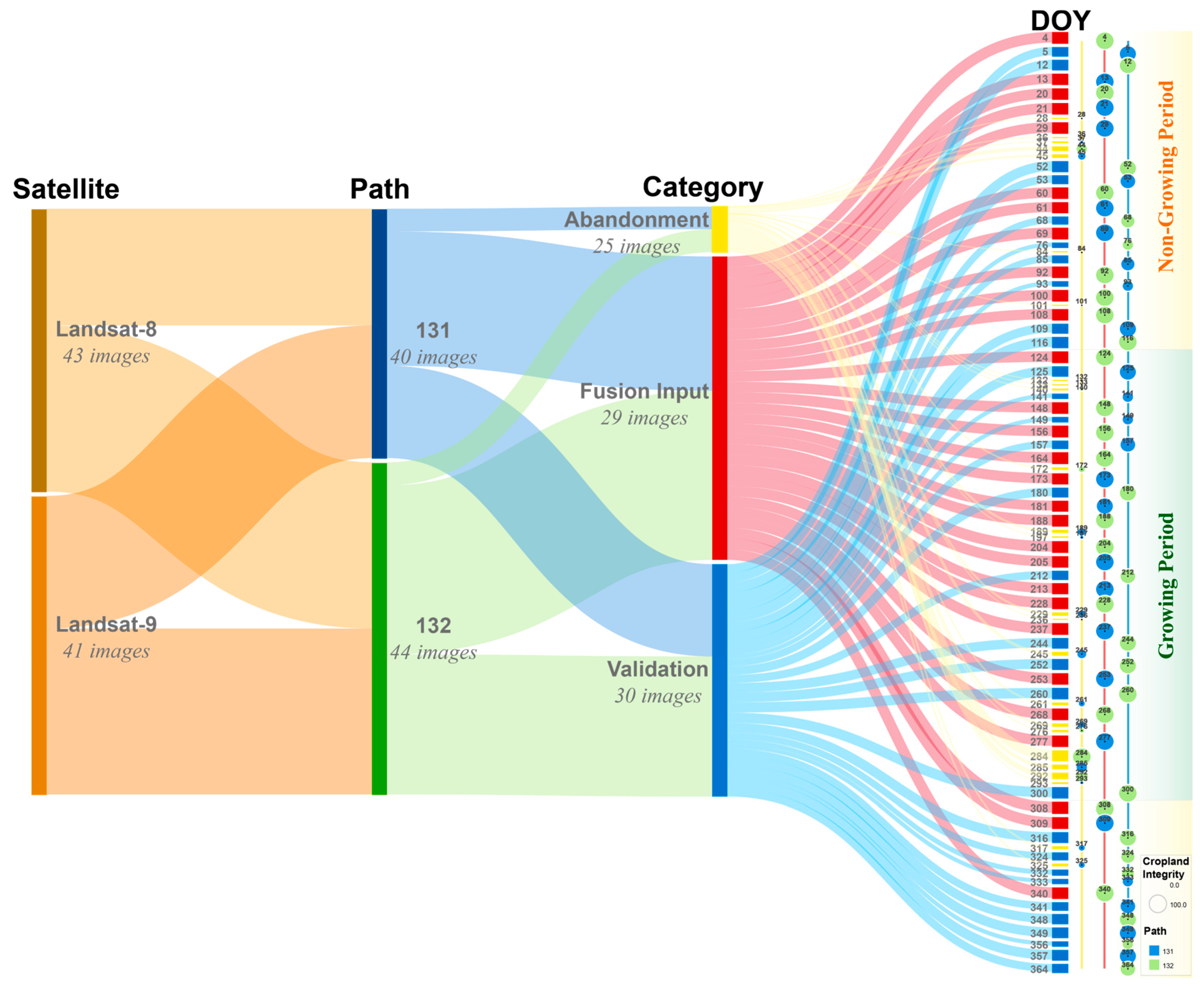
2.2. Input Remote Sensing Data

2.2.1. Land Use/Land Cover Data

The regional cropland for 2022 was identified by extracting the “Crops” category, corresponding to resampled class value 4, from the annual global map of land use and land cover (LULC) derived from European Space Agency (ESA) Sentinel-2 imagery at 10 m resolution [50]. LULC maps, generated by Impact Observatory, were developed using a deep learning U-Net model trained from scratch on over 5 billion hand-labeled datasets for land classification. These maps provide essential information, improving our understanding and quantification of the impacts of natural earth processes and human activities.

2.2.2. Surface Reflectance Data

To generate a high temporal resolution NDVI product, we utilized surface reflectance data from the MODerate-resolution imaging spectroradiometer (MODIS) sensor aboard NASA’s Terra (MOD) satellite. The satellite operates in a sun-synchronous orbit at an altitude of 705 km, with an acquisition schedule of 10:30 AM ± 15 min. The MOD09GA V6.1 product provides daily gridded Level-2G-lite data in sinusoidal projection, having undergone extensive accuracy assessments through global ground-validation campaigns [51]. Product comprises surface reflectance data for bands 1–7 at 500 m spatial resolution, and 1 km observation and geolocation statistics.

To generate high spatial resolution NDVI products, we utilized surface reflectance data from the Operational Land Imager (OLI) aboard Landsat-8 and OLI-2 aboard Landsat-9, launched by NASA and the United States Geological Survey (USGS). These satellites operate in a sun-synchronous orbit at an altitude of 705 km, with an acquisition schedule of 10:00 AM ± 15 min. The Landsat-8/9 Level 2 Collection 2 Science products provide surface reflectance data at 30 m spatial resolution with a 16-day revisit period, including five visible and near-infrared (VNIR) bands, two short-wave infrared (SWIR) bands, and quality assurance (QA) bands.

The Google Earth Engine (GEE) platform was used to access and preprocess the surface reflectance datasets from 1 January 2022 (DOY 001) to 31 December 2022 (DOY 365). Notably, the Terra spacecraft did not capture images between 12 October 2022 (DOY 285) and 19 October 2022 (DOY 292) due to the constellation exit manoeuvres [52].

Table 2. Summary of selected surface reflectance datasets and bands.

Datasets	Bands	$\mathbf{Wavelength} \mathbf{\left(}\mathbf{n}\mathbf{m}\mathbf{\right)}$	$\mathbf{Spatial} \mathbf{Resolution} \mathbf{\left(}\mathbf{m}\mathbf{\right)}$	$\mathbf{Temporal} \mathbf{Resolution} \mathbf{\left(}\mathbf{d}\mathbf{a}\mathbf{y}\mathbf{\right)}$
MODIS/061/MOD09GA	Red (1)	620–670	500	1
	Nir (2)	841–876
LANDSAT/LC08/C02/T1_L2LANDSAT/LC09/C02/T1_L2	Red (4)	630–680	30	16
	Nir (5)	845–885

summarizes the selected USGS datasets and bands, which underwent radiometric calibration, atmospheric correction, and surface reflectance calculations. The NDVI was derived from the Red and NIR bands of these datasets.

2.3. Data Preprocessing

The three surface reflectance datasets used are Level 2 remote sensing products, having undergone radiometric, atmospheric, geometric, and geographic corrections, as well as conversion from digital number to surface reflectance. Data preprocessing on the GEE platform focused primarily on cloud removal, data type conversion from bit-depth to normalized floating-point, and the application of the S-G filter on MOD09GA data. Subsequent data processing steps were executed in Python, encompassing nearest-neighbor resampling to 30 m resolution, cropping to cropland based on the LULC data, reprojection into the WGS 1984 UTM Zone 48N, and padding to dimensions of 8370 × 8370 × 2 (rows × columns × bands) to meet the fusion model’s input requirements.

2.3.1. MODIS Products

To enhance the temporal stability and spatial integrity of the input images, a pixel-level S-G filtering process was applied to the MOD09GA products [47]. Optimal filtering and noise reduction were achieved by setting the half-width of the smoothing window to 16 and the degree of fitting polynomials to 3.

2.3.2. Landsat Products

To ensure cropland integrity, discrimination and screening of Landsat-8/9 OLI/OLI-2 products were conducted. As illustrated in Figure 1, the entire SRB cropland area is fully covered by four Landsat-8/9 images, corresponding to two adjacent paths (Path 131 and Path 132) with a 7-day interval. Independent integrity assessments and functional classifications were then performed on the cropland depicted in the daily row-mosaic images from these paths.

All images captured along Path 131 or 132 in 2022 were merged into a single image using the maximum value approach. Cropland within the watershed was extracted based on LULC classification, where cropland pixels with valid values were assigned a class value of 1, and empty pixels were assigned a value of 0. This classification generated a basic cropland mask image for each path in 2022. The total cropland pixel count for each path was calculated by summing the pixels with a value of 1. Landsat-8/9 datasets, preprocessed on the GEE platform, underwent the same procedure to determine the cropland pixel counts for the day-scale row-mosaic images corresponding to their Julian day (DOY) and path. Cropland integrity for each image (%) was calculated by dividing the cropland pixel count for a specific DOY by the total cropland pixel count for that path.

Images with cropland integrity below 35% were classified as unavailable (abandonment). Those with cropland integrity above 95%—or above 90% for Path 131 due to limited availability—were selected as input images for the fusion model (fusion input). Images with cropland integrity between these thresholds were used as reference images to validate the fusion results (validation). Figure 3 illustrates all available Landsat-8/9 images from 2022.

2.4. Spatial and Temporal Fusion

The cropland distribution in the SRB is characterized by fragmented and scattered patterns with a highly complex cropping structure. Learning-based multidimensional image fusion methods often yield suboptimal results for this region, with reduced numerical accuracy and texture integrity. These limitations are primarily due to impurities in the training image samples, which include numerous scattered NODATA values. The Python-based VSDF model, by effectively capturing texture variations within the SRB’s complex planting structure, ensures temporal continuity at the pixel level.

According to Xu et al. [46], the core concepts of this method include utilizing abundant variation classification (AVC) to detect changes for spectral unmixing, guided by a relative reliability index (RRI) to optimize the prediction process. Additionally, feature-level fusion employs a Guided Filter to enhance edges and textures. With minimal input datasets—one fine-resolution image and a pair of coarse-resolution images—the key parameter, AVC, is estimated using a semi-empirical equation. This is followed by implementing the unsupervised K-Means clustering algorithm combined with spectral unmixing:

$${RMSE}_{{img}_1, {img}_2}={\displaystyle \frac{1}{B}}{\sum }_{b=0}^B\sqrt{{\displaystyle \frac{{\sum }_{n=1}^N{\left({img}_{1,n,b}-{img}_{2,n,b}\right)}^2}{N}}},$$

(1)

$$RRI={\displaystyle \frac{{RMSE}_{C_1,C_2}}{{RMSE}_{C_1,F_1}}},$$

(2)

$$AVC=\left(3-{\displaystyle \frac{1}{RRI}}\right)\times 2n_F,$$

(3)

where $RMSE$ represents the root mean squared error between two images (${img}_1$ and ${img}_2$); $B$ denotes the number of bands in the input image; $n,b$ indicates the value of pixel $n$ in band $b$, and $N$ is the total number of pixels in band $b$. $C_1$ and $C_2$ correspond to the pair of coarse-resolution input images (MODIS), while $F_1$ is the fine-resolution input images (Landsat) from the same DOY as $C_1$. The empirical parameter $n_F$ was set to 5.

2.5. Calculation of Vegetation Indexes

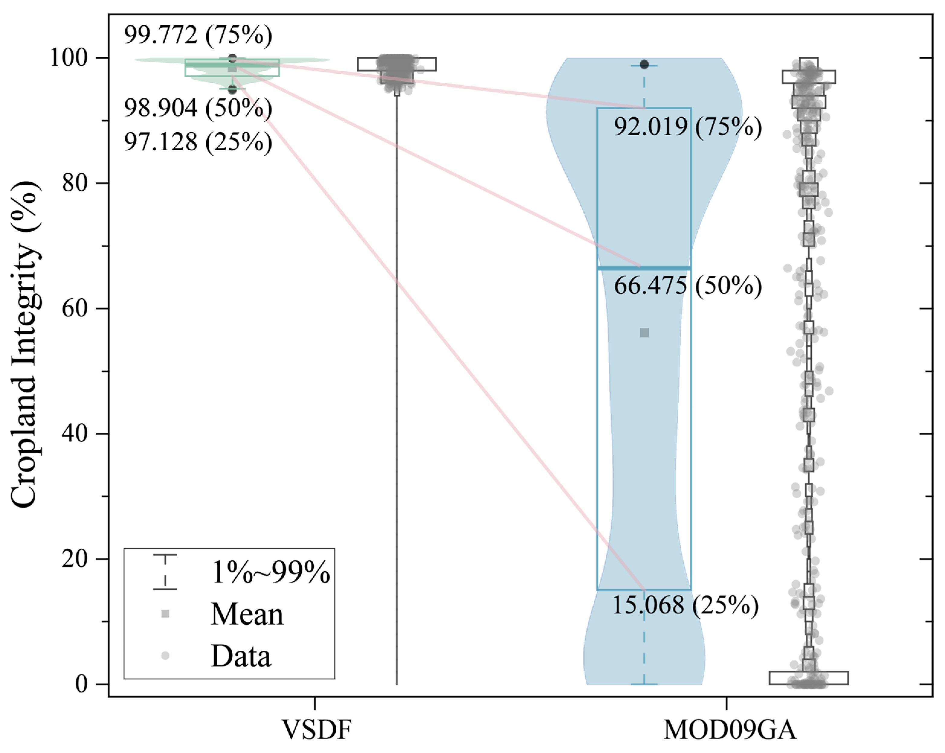
The satellite-based NDVI was calculated as follows, coded in Python:

$$NDVI={\displaystyle \frac{R_{NIR}-R_{Red}}{R_{NIR}+R_{Red}}},$$

(4)

where $R_{NIR}$ and $R_{Red}$ are the surface reflectance of band NIR and band Red, respectively. It is important to note that NDVI values should not be less than 0, as this study focuses on cropland in the SRB. NDVI values below 0 are not physically meaningful for vegetation assessment and could lead to misinterpretation, particularly in agricultural areas where vegetation cover is expected. After fusing and calculating daily images separately for Path 132 and Path 133, the results for the same day were mosaicked to create a complete 30 m daily NDVI dataset for the cropland in the SRB.

2.6. Validation

To comprehensively evaluate the accuracy of the results, the all-round performance assessment (APA) diagram proposed by Zhu et al. [53] was adopted. The APA includes four recommended indices across two domains: RMSE and average difference (AD) for spectral accuracy, and Robert’s edge (EDGE) and local binary patterns (LBP) for spatial accuracy. For all indices, the optimal value is 0, with values closer to zero indicating lower errors and higher accuracy. The indices were calculated as follows:

$$RMSE=\sqrt{{\displaystyle \frac{{\sum }_{n=1}^N{\left(F_i-R_i\right)}^2}{N}}},$$

(5)

$$AD={\displaystyle \frac{1}{N}}{\sum }_{n=1}^N\left(F_i-R_i\right),$$

(6)

$$EDGE=\left|D_{i,j}-D_{i+1,j+1}\right|+\left|D_{i,j+1}-D_{i+1,j}\right|,$$

(7)

$$\begin{array}{c}\hfill LBP=decimal\left(d_1{d}_2\dots d_8\right),\\ \hfill d_i=\left\{\begin{array}{cc}1& if D_i>D_C\\ 0& else\end{array}\right.,\end{array}$$

(8)

where $F_i$ is the value of valid pixel $i$ in the fused image, $R_i$ is the value of valid pixel $i$ in the reference image, $N$ is the total valid pixel number in the image, $D_{i,j}$ is the value of valid pixel at $i\mathrm{th}$ row and $j\mathrm{th}$ column, $D_i$ is the value of pixels surrounding the central pixel in a 3 × 3 moving window, and $D_C$ is the value of the central pixel. The term “decimal” refers to the conversion of binary digits to decimal numbers.

Also, the Pearson’s correlation coefficient (r) was calculated at pixel-level resolution to assess relationships between key variables, visualized through 2-D correlation plots:

$$\mathrm{r}={\displaystyle \frac{{\sum }_{n=1}^N{\left(F_i-\overline{F_i}\right)}^2{\left(R_i-\overline{R_i}\right)}^2}{\sqrt{{\sum }_{n=1}^N{\left(F_i-\overline{F_i}\right)}^2{\left(R_i-\overline{R_i}\right)}^2}}},$$

(9)

where $\overline{F_i}$ is the average value of all valid pixels in the fused image, and $\overline{R_i}$ is the average value of all valid pixels in the reference image.

3. Results

The reconstructed daily NDVI datasets offer critical insights into vegetation responses to climate and environmental changes. Researchers can use this dataset to develop refined planting structure classification maps for the SRB, analyze the temporal and spatial dynamics of crop growth, and investigate vegetation responses under changing conditions. The dataset, available in TIFF format at the National Tibetan Plateau Data Center [54], can be accessed and processed using platforms such as standard GIS software, Python, MATLAB, or equivalent tools capable of handling TIFF data. The reconstructed NDVI dataset is stored in the Int16 data type to optimize storage efficiency and processing speed while maintaining precision for high-resolution analysis. Users must multiply downloaded NDVI values by a scale factor of 0.0001 to convert the data from Int16 to Float32 for accurate interpretation.

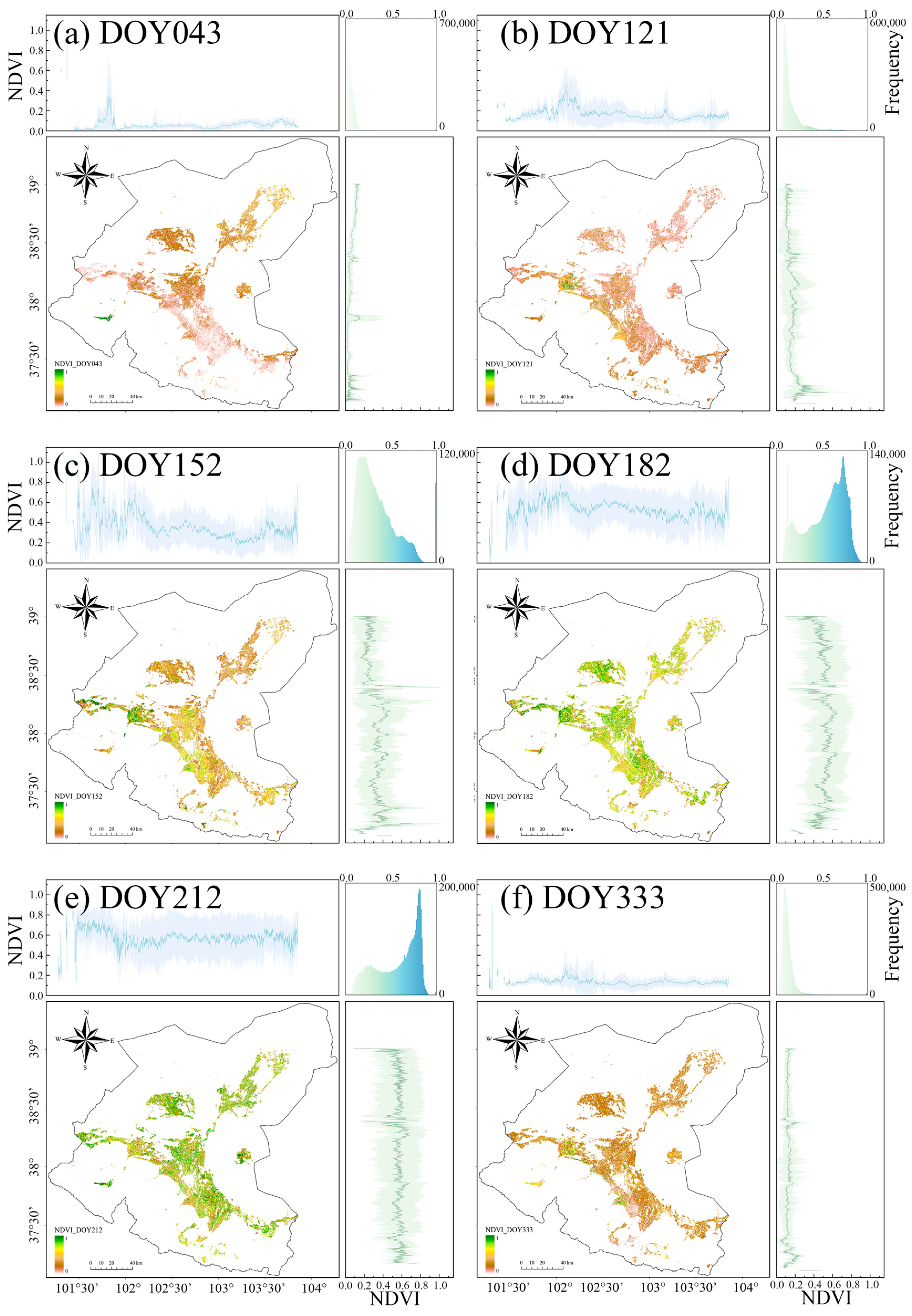
3.1. Regional Reconstruction NDVI

Figure 4 illustrates the cropland integrity of the region, comparing the reconstructed NDVI after fusion with the initial MOD09GA NDVI. The average cropland integrity rate of the reconstructed NDVI products reached 98.50%, a significant improvement over the 56.15% integrity of the original MOD09GA NDVI, representing an average increase of 42.35%.

Figure 5a–h displays the spatial distributions of the original MOD09GA NDVI and the reconstructed NDVI for two specific days. Visual analysis highlights significant gaps and data losses in the original images. Although the MOD09GA NDVI was resampled to a 30 m spatial resolution, texture details are severely degraded, with minimal spatial differentiation between fields, failing to achieve effective scaling. In contrast, the reconstructed NDVI product successfully fills gaps caused by cloud contamination and missing data. It also preserves high-quality texture details at a 30 m resolution, enabling the capture of refined spatial information across extended time series.

3.2. Quantitative Evaluation of Reconstructed NDVI

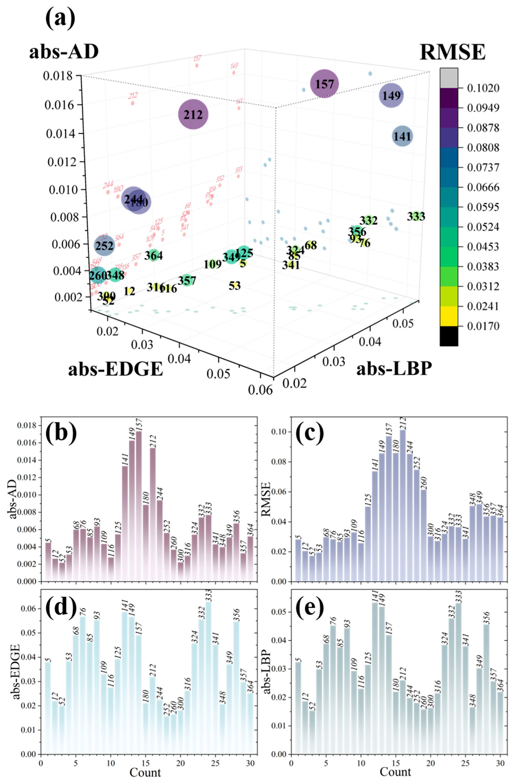
3.2.1. Evaluation Based on 3D-APA Diagram

The accuracy of the reconstructed NDVI products was validated using 30 selected Landsat images. The absolute APA (abs-APA) metrics for all four accuracy indices are presented in Figure 6. For visual clarity, both the 3D-APA diagram and the absolute values of the original APA performance metrics are displayed, where lower bar heights indicate better performance. The validated NDVI values, all within acceptable error ranges, exhibit distinct patterns corresponding to two periods: the growing period (DOY 121–304) and the non-growing period (remaining days).

Figure 6a illustrates the performance of the four accuracy indices in reconstructing NDVI. Images captured during the non-growing period generally exhibit lower error values and better results compared to those from the growing period. However, the accuracy for DOY 141, 149, 157, and 212 (21 May, 29 May, 6 June, and 31 July) is notably poorer, corresponding to critical growth stages of various crops under complex planting structures.

Quantitative analysis of spectral accuracy across all 30 validation images (Figure 6b,c) reveals average abs-AD and RMSE values of 0.0064 and 0.0466, respectively. During the growing season, these averages increase to 0.0098 and 0.0746, while in the non-growing season, they decrease to 0.0048 and 0.0326. Analysis of spatial accuracy (Figure 6d,e shows average abs-EDGE and abs-LBP values of 0.0373 and 0.0317, respectively. During the growing season, the averages are 0.0329 and 0.0296, compared to 0.0394 and 0.0327 in the non-growing season.

Comparing the spectral and spatial domains, we observe distinct trends during the growing season as crops progress through phenological stages of growth, maturity, and harvest. Errors in the spectral accuracy domain initially increase and then decrease, while errors in the spatial accuracy domain follow an inverse trend, decreasing first and then increasing. During the non-growing season, both domains exhibit an “opposite trend” of trade-offs. Notably, all four error indices reach a minimum on DOY 12, 52, and 300 (12 January, 21 February, and 27 October), indicating the superior quality of the reconstructed NDVI images for these days. Furthermore, errors for all other validation images remain within acceptable ranges, demonstrating the effectiveness of the VSDF model in fusing and deriving high-resolution, diurnal-scale NDVI with reliable spectral and spatial predictions.

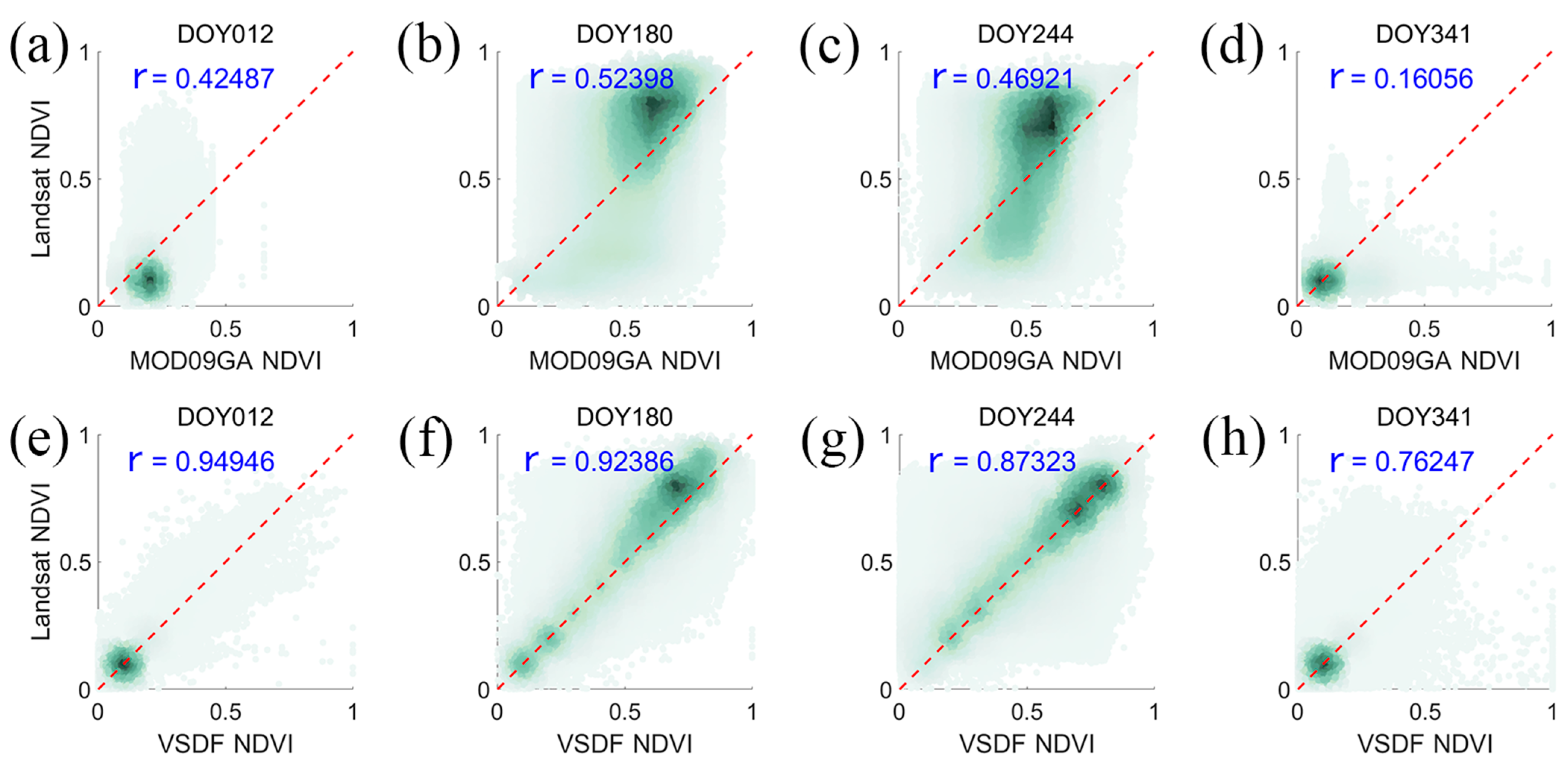
3.2.2. Comparison with Original MOD09GA NDVI

To fully evaluate the reliability of the reconstructed NDVI from VSDF-based images, we compared the full-pixel scale NDVI derived from MOD09GA, Landsat, and VSDF images for the same period. Due to significant gaps and low cropland integrity in the MOD09GA NDVI dataset, a direct comparison of spectral or spatial domain errors between the original MOD09GA NDVI and the reconstructed VSDF NDVI is unsuitable. Image defects in the MOD09GA NDVI reduce the number of pixels included in spectral error calculations, producing artificially low error values. Additionally, the fragmented cropland structure is poorly represented, with texture variations often unaccounted for, resulting in a misleading zero error in spatial calculations based on sliding windows. To address these limitations, we assessed accuracy using the Pearson correlation coefficient (r) of full-pixel effective values derived from Landsat NDVI validation images to compare the performance of the reconstructed VSDF NDVI with the MOD09GA NDVI.

Figure 7 presents accuracy estimates for MOD09GA NDVI and VSDF NDVI across four representative days from the growing and non-growing seasons. For the 30 validation images of VSDF NDVI was 0.7511, with averages of 0.7047 during the non-growing season and 0.8439 during the growing season. In contrast, the MOD09GA NDVI exhibits an overall r-mean of 0.5790, with averages of 0.5903 during the non-growing season and 0.5566 during the growing season. This represents a relative accuracy improvement of 49.88% for the VSDF NDVI, with improvements of 45.01% and 59.64% in the non-growing and growing seasons, respectively. The highest r for VSDF NDVI was observed on DOY 012 during the non-growing season (0.9495) and on DOY 212 during the growing season (0.9337). The increment from MOD09GA NDVI to VSDF NDVI during the non-growing season occurred on DOY 341, increasing from 0.1606 to 0.7625, an absolute improvement of 0.6019, and a relative increase of 374.88%. Similarly, the largest increment during the growing season is on DOY 149, with r increasing from 0.3605 to 0.7918, an absolute improvement of 0.4312, and a relative increase of 119.61%. In summary, the reconstructed NDVI results demonstrated significantly higher accuracy, with errors consistently remaining within acceptable ranges.

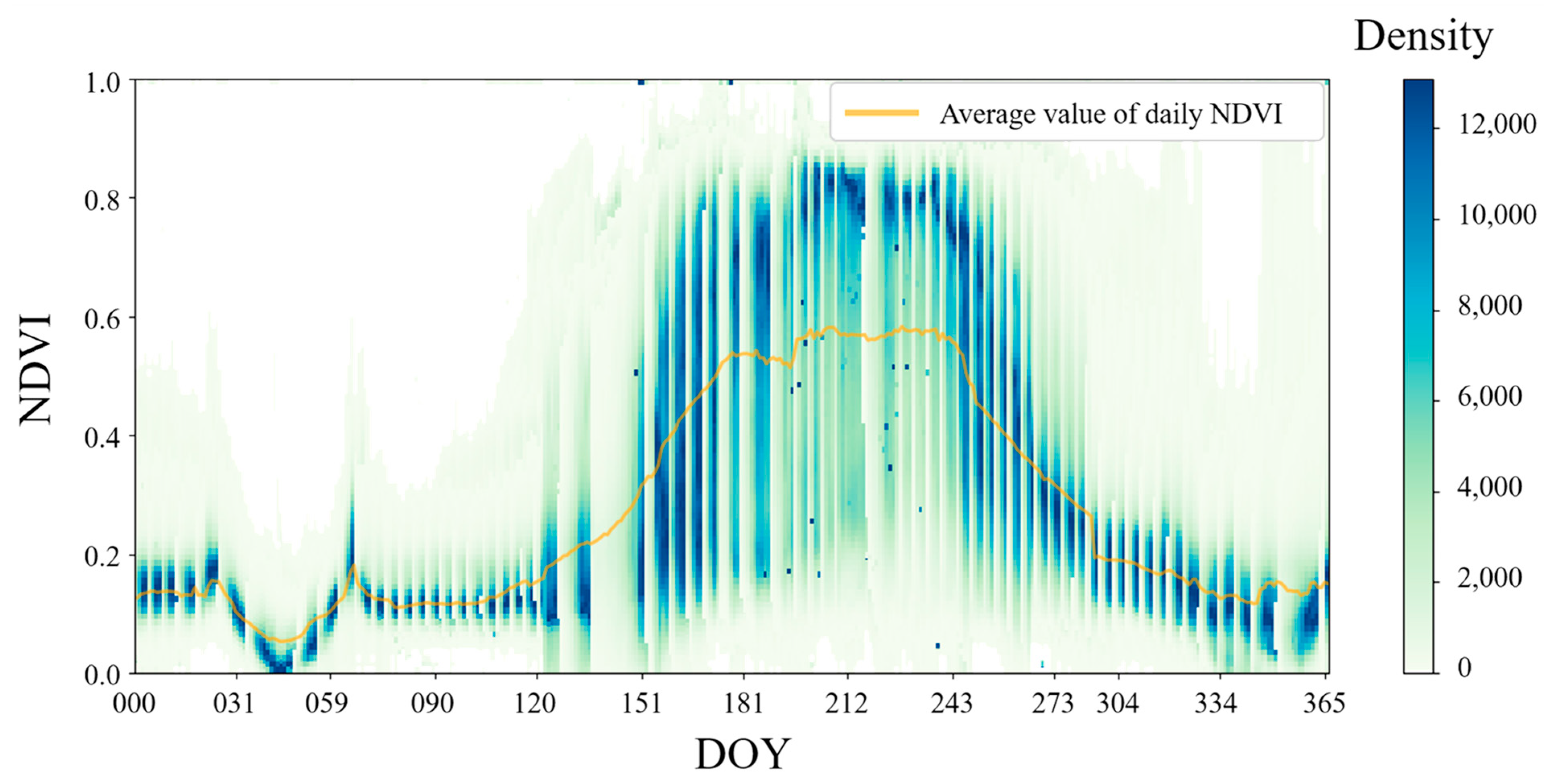
3.3. Daily Temporal–Spatial Distribution

Figure 8 and Figure 9 illustrate VSDF NDVI change curves and data distributions, highlighting significant spatiotemporal variations throughout 2022. The daily NDVI variation within the watershed demonstrates pronounced temporal and spatial heterogeneity. Temporally, NDVI values were lowest in mid-February (DOY 043) before rising and stabilizing in early March. With the growing season starting on 1 May (DOY 121), NDVI values increased as major crops grew, peaking during the maturity and harvest periods in July (DOY 182) and August (after DOY 212). By September, following the harvest of bulk crops like corn, NDVI values began to decline. After 31 October (DOY 304), marking the onset of the non-growing season, NDVI values stabilized. During this period, short-cycle forage grasses were planted, causing average NDVI values to fluctuate around 0.15. In February, forage harvests reduced NDVI values; however, winter wheat planted the previous year continued to grow, maintaining a regional average NDVI of 0.06. Yet the data distribution is concentrated in the uncultivated area, where the value is 0.

The spatial distribution of NDVI across different days and within the same day in the watershed reveals significant differentiation. Comparing spatial distribution maps from the non-growing and growing seasons allows for an intuitive assessment of crop growth stages and planting structures, including forage grass, winter wheat, spring wheat, and corn, aligned with their respective planting timelines. This highlights the effectiveness of the 30 m daily NDVI product for SRB cropland in 2022 in capturing the spatial distribution and growth patterns of various crops. The dataset enables large-scale crop status monitoring under complex planting structures across multiple stages, providing a high-efficiency, high-precision foundation for advancing precision agriculture in the SRB.

4. Discussion

4.1. Optimized Image Selection Strategy for NDVI Fusion

In this study, Landsat images from two adjacent paths (Path 131 and Path 132) were selected based on cropland integrity rather than conventional cloud cover filtering [55,56]. This approach ensured the retention of more usable imagery during fusion, particularly for agricultural regions, which are often fragmented in large-scale remote sensing studies. By excluding images with extensive missing data and retaining only those with cropland integrity exceeding 95%, the fusion results maintained spatial and temporal consistency. This selection method also addressed a common challenge in large river basins, where multiple Landsat paths introduce temporal discrepancies in image acquisition [57,58].

A key limitation of the VSDF model is its reliance on minimal input—two coarse-resolution and one fine-resolution image—without a time-series prediction mechanism based on time-series images or deep learning networks [59,60,61]. While effective for short intervals, its accuracy declines over extended gaps. After DOY 310, available imagery dropped sharply (Figure 3), reducing prediction reliability. Despite ensuring a 1-day difference between adjacent paths and maintaining a 5-day near-time interval, same-path gaps often exceeded 16 days, surpassing the 15-day threshold for reliable fusion [13,46]. Addressing this limitation requires integrating additional datasets (e.g., Sentinel-2, Landsat 5–7) or refining model parameters to improve robustness for long-term NDVI reconstruction.

Future investigations will incorporate remaining spectral bands from daily MOD09GA datasets (500 m resolution) into 30 m daily surface reflectance reconstructions to support evapotranspiration retrieval. The selection of MOD09GA over higher-resolution MOD09GQ (250 m resolution, limited to red and near-infrared spectral regions) minimizes inter-sensor variability through standardized data inputs. While MOD09GQ offers enhanced spatial texture characterization, using MOD09GA aligns better with the input parameters and empirical calibration methods intrinsic to the VSDF model. This strategic choice further validates the robust performance of the VSDF model even under substantial spatial downscaling scenarios.

4.2. Enhanced Accuracy Assessment Through 3D-APA Analysis

The integration of additional parameters into the 3D-APA (3D adaptive parameter adjustment) framework enabled a more comprehensive error assessment [53], further validating the VSDF model’s performance. Results demonstrate the model’s high spectral accuracy, particularly during the non-growing season, where it effectively captured subtle reflectance variations in land cover dominated by bare soil and sparse vegetation, such as forage grass. This capability enhances high-frequency surface dynamics monitoring, crop phenology tracking, and planting structure analysis [62,63,64].

During the growing season, the model maintained strong spatial accuracy, preserving fine-scale texture details despite complex vegetation dynamics. This precision is essential for distinguishing crop types, monitoring growth trends, and assessing agricultural productivity [65,66,67,68,69]. The reconstructed NDVI images consistently fell within acceptable error thresholds, as indicated by validation metrics such as abs-AD (0.0064), RMSE (0.0466), abs-EDGE (0.0373), and abs-LBP (0.0317). These findings confirm the dataset’s reliability for high-resolution spatiotemporal applications, supporting precision agriculture in the SRB.

Overall, the VSDF model’s ability to balance spectral and spatial accuracy across different seasons ensures robust retrieval of fine-scale surface characteristics. This strength facilitates effective crop differentiation and management throughout various growth stages, reinforcing its utility for large-scale agricultural monitoring and decision-making.

4.3. Spatiotemporal Visualization of Crop Growth Dynamics

The reconstructed high-resolution daily NDVI dataset provides valuable insights into crop phenology and land surface changes at an unprecedented temporal granularity. The observed temporal trends in NDVI correspond well with the established crop growth cycles in the SRB [49,70,71,72,73]. During the early months of the year, NDVI values remain low, reflecting minimal vegetation cover, as most fields lay fallow except for winter wheat and sparse forage grasses. The rise in NDVI from early March signals the onset of pre-planting activities, including soil preparation and the initial stages of winter wheat development. As the primary growing season begins on 1 May (DOY 121), NDVI values increase substantially, capturing the emergence and expansion of major crops such as spring wheat and corn.

The peak NDVI values observed in July (DOY 182) and August (after DOY 212) align with the maturity and harvest periods of key crops. This period exhibits the highest photosynthetic activity, with NDVI values nearing saturation [74,75]. Following the primary harvest in September, NDVI declines, reflecting the removal of biomass from harvested fields. However, the dataset also captures short-cycle forage grass cultivation during the non-growing season, which contributes to NDVI fluctuations of around 0.15 after 31 October (DOY 304). Notably, winter wheat planted the previous year maintains a higher NDVI (~0.20) than non-cultivated areas, indicating its role in stabilizing land surface conditions during winter months (around DOY 043, Figure 8).

The dataset’s 30 m spatial resolution reveals heterogeneous cropland management and planting structures, distinguishing fragmented forage grass plots, contiguous wheat fields, and intercropped areas. During the non-growing season, spatial NDVI patterns vary significantly, reflecting diverse land-use practices such as rotational cropping and winter cover crops. Compared to coarser NDVI products, this dataset significantly advances the capability to:

Improved crop differentiation—High spatial resolution facilitates accurate identification of planting structures and land-use classification.

Detailed phenological tracking—Capturing fine-scale NDVI variations supports precise monitoring of crop growth and seasonal transitions.

Optimized agricultural management—The dataset informs irrigation, fertilization, and yield estimation strategies, supporting sustainable farming.

This dataset marks a significant advancement in agricultural monitoring, providing a robust foundation for researchers, policymakers, and farmers to enhance productivity and sustainability.

5. Conclusions

This study reconstructs a high-resolution (30 m) daily NDVI dataset for cropland in the SRB in 2022 using S-G filtering and the VSDF model. By prioritizing cropland integrity over traditional cloud cover filtering, the dataset ensures more spatial and temporal consistency, addressing challenges in multi-path Landsat acquisitions. It significantly improves upon MOD09GA NDVI, achieving a 98.50% cropland integrity rate (a 42.35% increase) and an average r-mean of 0.7511 (49.88% higher), with 3-D validation metrics confirming high accuracy. The dataset enables detailed crop phenology and land-use monitoring, capturing key growth stages from early development in March to peak biomass in July and post-harvest senescence. It effectively distinguishes spatially heterogeneous planting structures and reflects rotational cropping and winter cover crop practices during the non-growing season.

The reliable methodology for high-precision NDVI reconstruction provided by the study supports precision agriculture and land management. Future research should integrate Sentinel-2 imagery for enhanced temporal consistency and explore NDVI coupling with climatic and soil moisture data to deepen insights into environmental drivers of vegetation dynamics. Continued refinement of high-resolution NDVI methods will advance data-driven agricultural monitoring.

References

1. Gao, Y.-Y.; He, J.; Li, X.-H.; Li, J.-H.; Wu, H.; Wen, T.; Li, J.; Hao, G.-F.; Yoon, J. Fluorescent Chemosensors Facilitate the Visualization of Plant Health and Their Living Environment in Sustainable Agriculture. Chem. Soc. Rev. 2024, 53, 6992–7090. [Google Scholar] [CrossRef] [PubMed]
2. Down-to-Earth Drought Resistance. Nat. Plants 2024, 10, 525–526. [CrossRef] [PubMed]
3. Nogrady, B. How to Address Agriculture’s Water Woes. Nature 2024, 630, S26–S27. [Google Scholar] [CrossRef]
4. Li, X.; Wang, Y.; Zhao, Y.; Zhai, J.; Liu, Y.; Han, S.; Liu, K. Research on the Impact of Climate Change and Human Activities on the NDVI of Arid Areas—A Case Study of the Shiyang River Basin. Land 2024, 13, 533. [Google Scholar] [CrossRef]
5. Grayson, M. Agriculture and Drought. Nature 2013, 501, S1. [Google Scholar] [CrossRef]
6. Christou, A.; Beretsou, V.G.; Iakovides, I.C.; Karaolia, P.; Michael, C.; Benmarhnia, T.; Chefetz, B.; Donner, E.; Gawlik, B.M.; Lee, Y.; et al. Sustainable Wastewater Reuse for Agriculture. Nat. Rev. Earth Environ. 2024, 5, 504–521. [Google Scholar] [CrossRef]
7. Mooney, S.J.; Castrillo, G.; Cooper, H.V.; Bennett, M.J. Root–Soil–Microbiome Management Is Key to the Success of Regenerative Agriculture. Nat. Food 2024, 5, 451–453. [Google Scholar] [CrossRef]
8. Rouse, J.W., Jr.; Haas, R.H.; Deering, D.W.; Schell, J.A. Monitoring the Vernal Advancement and Retrogradation (Green Wave Effect) of Natural Vegetation; Texas A&M University: College Station, TX, USA, 1973. [Google Scholar]
9. Rouse, J.W., Jr.; Haas, R.H.; Deering, D.W.; Schell, J.A.; Harlan, J.C. Monitoring the Vernal Advancement and Retrogradation (Green Wave Effect) of Natural Vegetation; Texas A&M University: College Station, TX, USA, 1974. [Google Scholar]
10. Tucker, C.J. Red and Photographic Infrared Linear Combinations for Monitoring Vegetation. Remote Sens. Environ. 1979, 8, 127–150. [Google Scholar] [CrossRef]
11. Chen, D.; Hu, H.; Liao, C.; Ye, J.; Bao, W.; Mo, J.; Wu, Y.; Dong, T.; Fan, H.; Pei, J. Crop NDVI Time Series Construction by Fusing Sentinel-1, Sentinel-2, and Environmental Data with an Ensemble-Based Framework. Comput. Electron. Agric. 2023, 215, 108388. [Google Scholar] [CrossRef]
12. Zhang, C.; Yang, Z.; Di, L.; Yu, E.G.; Zhang, B.; Han, W.; Lin, L.; Guo, L. Near-Real-Time MODIS-Derived Vegetation Index Data Products and Online Services for CONUS Based on NASA LANCE. Sci. Data 2022, 9, 477. [Google Scholar] [CrossRef]
13. Gu, Z.; Chen, J.; Chen, Y.; Qiu, Y.; Zhu, X.; Chen, X. Agri-Fuse: A Novel Spatiotemporal Fusion Method Designed for Agricultural Scenarios with Diverse Phenological Changes. Remote Sens. Environ. 2023, 299, 113874. [Google Scholar] [CrossRef]
14. Farbo, A.; Sarvia, F.; De Petris, S.; Basile, V.; Borgogno-Mondino, E. Forecasting Corn NDVI through AI-Based Approaches Using Sentinel 2 Image Time Series. ISPRS J. Photogramm. Remote Sens. 2024, 211, 244–261. [Google Scholar] [CrossRef]
15. MODIS Terra Daily NDSI|Earth Engine Data Catalog. Available online: https://developers.google.cn/earth-engine/datasets/catalog/MODIS_MOD09GA_006_NDSI (accessed on 15 July 2024).
16. Lyapustin, A. MODIS/Terra+Aqua Vegetation Index from MAIAC, Daily L3 Global 0.05Deg CMG V061 2023. Available online: https://lpdaac.usgs.gov/products/mcd19a3cmgv061 (accessed on 14 July 2024).
17. Li, H.; Cao, Y.; Xiao, J.; Yuan, Z.; Hao, Z.; Bai, X.; Wu, Y.; Liu, Y. A Daily Gap-Free Normalized Difference Vegetation Index Dataset from 1981 to 2023 in China. Sci. Data 2024, 11, 527. [Google Scholar] [CrossRef]
18. Xiong, C.; Ma, H.; Liang, S.; He, T.; Zhang, Y.; Zhang, G.; Xu, J. Improved Global 250 m 8-Day NDVI and EVI Products from 2000–2021 Using the LSTM Model. Sci. Data 2023, 10, 800. [Google Scholar] [CrossRef]
19. Didan, K. MODIS/Aqua Vegetation Indices 16-Day L3 Global 250m SIN Grid V061 2021. Available online: https://lpdaac.usgs.gov/products/myd13q1v061 (accessed on 14 July 2024).
20. Kidner, D.; Dorey, M.; Smith, D. What’s the Point? Interpolation and Extrapolation with a Regular Grid DEM. In Proceedings of the 4th International Conference on GeoComputation, Fredericksburg, VA, USA, 25–28 July 1999. [Google Scholar]
21. Savitzky, A.; Golay, M.J.E. Smoothing and Differentiation of Data by Simplified Least Squares Procedures. Anal. Chem. 1964, 36, 1627–1639. [Google Scholar] [CrossRef]
22. Kalman, R.E. A New Approach to Linear Filtering and Prediction Problems. J. Basic Eng. 1960, 82, 35–45. [Google Scholar] [CrossRef]
23. Kalman, R.E.; Bucy, R.S. New Results in Linear Filtering and Prediction Theory. J. Basic Eng. 1961, 83, 95–108. [Google Scholar] [CrossRef]
24. Morlet, J.; Arens, G.; Fourgeau, E.; Glard, D. Wave Propagation and Sampling Theory—Part I: Complex Signal and Scattering in Multilayered Media. Geophysics 1982, 47, 203–221. [Google Scholar] [CrossRef]
25. Grossmann, A.; Morlet, J. Decomposition of Hardy Functions into Square Integrable Wavelets of Constant Shape. SIAM J. Math. Anal. 1984, 15, 723–736. [Google Scholar] [CrossRef]
26. Li, M.; Cao, S.; Zhu, Z.; Wang, Z.; Myneni, R.B.; Piao, S. Spatiotemporally Consistent Global Dataset of the GIMMS Normalized Difference Vegetation Index (PKU GIMMS NDVI) from 1982 to 2022. Earth Syst. Sci. Data 2023, 15, 4181–4203. [Google Scholar] [CrossRef]
27. Wu, P.; Shen, H.; Zhang, L.; Göttsche, F.-M. Integrated Fusion of Multi-Scale Polar-Orbiting and Geostationary Satellite Observations for the Mapping of High Spatial and Temporal Resolution Land Surface Temperature. Remote Sens. Environ. 2015, 156, 169–181. [Google Scholar] [CrossRef]
28. Dong, W.; Fu, F.; Shi, G.; Cao, X.; Wu, J.; Li, G.; Li, X. Hyperspectral Image Super-Resolution via Non-Negative Structured Sparse Representation. IEEE Trans. Image Process. 2016, 25, 2337–2352. [Google Scholar] [CrossRef] [PubMed]
29. Dian, R.; Fang, L.; Li, S. Hyperspectral Image Super-Resolution via Non-Local Sparse Tensor Factorization. In Proceedings of the IEEE Conference on Computer Vision and Pattern Recognition, Honolulu, HI, USA, 21–26 July 2017; pp. 5344–5353. [Google Scholar]
30. Tan, Z.; Yue, P.; Di, L.; Tang, J. Deriving High Spatiotemporal Remote Sensing Images Using Deep Convolutional Network. Remote Sens. 2018, 10, 1066. [Google Scholar] [CrossRef]
31. Song, H.; Liu, Q.; Wang, G.; Hang, R.; Huang, B. Spatiotemporal Satellite Image Fusion Using Deep Convolutional Neural Networks. IEEE J. Sel. Top. Appl. Earth Obs. Remote Sens. 2018, 11, 821–829. [Google Scholar] [CrossRef]
32. Liu, X.; Liu, Q.; Wang, Y. Remote Sensing Image Fusion Based on Two-Stream Fusion Network. Inf. Fusion 2020, 55, 1–15. [Google Scholar] [CrossRef]
33. Yang, Y.; Tu, W.; Huang, S.; Lu, H.; Wan, W.; Gan, L. Dual-Stream Convolutional Neural Network with Residual Information Enhancement for Pansharpening. IEEE Trans. Geosci. Remote Sens. 2021, 60, 5402416. [Google Scholar] [CrossRef]
34. Ozcelik, F.; Alganci, U.; Sertel, E.; Unal, G. Rethinking CNN-Based Pansharpening: Guided Colorization of Panchromatic Images via GANs. IEEE Trans. Geosci. Remote Sens. 2020, 59, 3486–3501. [Google Scholar] [CrossRef]
35. Tan, Z.; Gao, M.; Li, X.; Jiang, L. A Flexible Reference-Insensitive Spatiotemporal Fusion Model for Remote Sensing Images Using Conditional Generative Adversarial Network. IEEE Trans. Geosci. Remote Sens. 2022, 60, 5601413. [Google Scholar] [CrossRef]
36. Yuan, Q.; Shen, H.; Li, T.; Li, Z.; Li, S.; Jiang, Y.; Xu, H.; Tan, W.; Yang, Q.; Wang, J.; et al. Deep Learning in Environmental Remote Sensing: Achievements and Challenges. Remote Sens. Environ. 2020, 241, 111716. [Google Scholar] [CrossRef]
37. Wang, Z.; Ma, Y.; Zhang, Y. Review of Pixel-Level Remote Sensing Image Fusion Based on Deep Learning. Inf. Fusion 2023, 90, 36–58. [Google Scholar] [CrossRef]
38. Ao, Z.; Sun, Y.; Pan, X.; Xin, Q. Deep Learning-Based Spatiotemporal Data Fusion Using a Patch-to-Pixel Mapping Strategy and Model Comparisons. IEEE Trans. Geosci. Remote Sens. 2022, 60, 5407718. [Google Scholar] [CrossRef]
39. Sun, C.; Shrivastava, A.; Singh, S.; Gupta, A. Revisiting Unreasonable Effectiveness of Data in Deep Learning Era. In Proceedings of the IEEE International Conference on Computer Vision, Venice, Italy, 22–29 October 2017; pp. 843–852. [Google Scholar]
40. Gao, F.; Masek, J.; Schwaller, M.; Hall, F. On the Blending of the Landsat and MODIS Surface Reflectance: Predicting Daily Landsat Surface Reflectance. IEEE Trans. Geosci. Remote Sens. 2006, 44, 2207–2218. [Google Scholar] [CrossRef]
41. Zhang, W.; Li, A.; Jin, H.; Bian, J.; Zhang, Z.; Lei, G.; Qin, Z.; Huang, C. An Enhanced Spatial and Temporal Data Fusion Model for Fusing Landsat and MODIS Surface Reflectance to Generate High Temporal Landsat-Like Data. Remote Sens. 2013, 5, 5346–5368. [Google Scholar] [CrossRef]
42. Zhu, X.; Helmer, E.H.; Gao, F.; Liu, D.; Chen, J.; Lefsky, M.A. A Flexible Spatiotemporal Method for Fusing Satellite Images with Different Resolutions. Remote Sens. Environ. 2016, 172, 165–177. [Google Scholar] [CrossRef]
43. Gao, H.; Zhu, X.; Guan, Q.; Yang, X.; Yao, Y.; Zeng, W.; Peng, X. cuFSDAF: An Enhanced Flexible Spatiotemporal Data Fusion Algorithm Parallelized Using Graphics Processing Units. IEEE Trans. Geosci. Remote Sens. 2022, 60, 4403016. [Google Scholar] [CrossRef]
44. Zhukov, B.; Oertel, D.; Lanzl, F.; Reinhackel, G. Unmixing-Based Multisensor Multiresolution Image Fusion. IEEE Trans. Geosci. Remote Sens. 1999, 37, 1212–1226. [Google Scholar] [CrossRef]
45. Wu, M.; Niu, Z.; Wang, C.; Wu, C.; Wang, L. Use of MODIS and Landsat Time Series Data to Generate High-Resolution Temporal Synthetic Landsat Data Using a Spatial and Temporal Reflectance Fusion Model. J. Appl. Remote Sens. 2012, 6, 063507. [Google Scholar] [CrossRef]
46. Xu, C.; Du, X.; Yan, Z.; Zhu, J.; Xu, S.; Fan, X. VSDF: A Variation-Based Spatiotemporal Data Fusion Method. Remote Sens. Environ. 2022, 283, 113309. [Google Scholar] [CrossRef]
47. Chen, J.; Jönsson, P.; Tamura, M.; Gu, Z.; Matsushita, B.; Eklundh, L. A Simple Method for Reconstructing a High-Quality NDVI Time-Series Data Set Based on the Savitzky–Golay Filter. Remote Sens. Environ. 2004, 91, 332–344. [Google Scholar] [CrossRef]
48. Shi, J.; Shi, P.; Li, X.; Wang, Z.; Xu, A. Spatial and temporal variability of ecosystem services in the Shiyang River Basin and its multi-scale influencing factors. Prog. Geogr. 2024, 43, 276–289. [Google Scholar] [CrossRef]
49. Yang, X.; Shi, X.; Zhang, Y.; Tian, F.; Ortega-Farias, S. Response of Evapotranspiration (ET) to Climate Factors and Crop Planting Structures in the Shiyang River Basin, Northwestern China. Remote Sens. 2023, 15, 3923. [Google Scholar] [CrossRef]
50. Karra, K.; Kontgis, C.; Statman-Weil, Z.; Mazzariello, J.C.; Mathis, M.; Brumby, S.P. Global Land Use/Land Cover with Sentinel 2 and Deep Learning. In Proceedings of the 2021 IEEE International Geoscience and Remote Sensing Symposium IGARSS, Brussels, Belgium, 11–16 July 2021; pp. 4704–4707. [Google Scholar]
51. Vermote, E. MODIS/Terra Surface Reflectance Daily L2G Global 1 km and 500 m SIN Grid 2021. Available online: https://lpdaac.usgs.gov/products/mod09gav061 (accessed on 14 April 2024).
52. Schwenger, S.; MODIS and VIIRS Characterization Support Teams, NASA GSFC. MODIS and VIIRS Instrument Operations Status. In Proceedings of the 2023 MODIS/VIIRS Science Team Meeting, College Park, MD, USA, 1–4 May 2023; Available online: https://modis.gsfc.nasa.gov/sci_team/meetings/202305/presentations/cal/01_Schwenger_MODISVIIRSInstOps.pdf (accessed on 2 August 2024).
53. Zhu, X.; Zhan, W.; Zhou, J.; Chen, X.; Liang, Z.; Xu, S.; Chen, J. A Novel Framework to Assess All-Round Performances of Spatiotemporal Fusion Models. Remote Sens. Environ. 2022, 274, 113002. [Google Scholar] [CrossRef]
54. Mu, P. A Daily 30 m NDVI Product of Cropland in the Shiyang River Basin, Northwestern China of 2022. Available online: https://cstr.cn/18406.11.Terre.tpdc.302191 (accessed on 7 March 2025).
55. Xu, H.; Sun, H.; Xu, Z.; Wang, Y.; Zhang, T.; Wu, D.; Gao, J. kNDMI: A Kernel Normalized Difference Moisture Index for Remote Sensing of Soil and Vegetation Moisture. Remote Sens. Environ. 2025, 319, 114621. [Google Scholar] [CrossRef]
56. Ebrahimy, H.; Yu, T.; Zhang, Z. Developing a Spatiotemporal Fusion Framework for Generating Daily UAV Images in Agricultural Areas Using Publicly Available Satellite Data. ISPRS J. Photogramm. Remote Sens. 2025, 220, 413–427. [Google Scholar] [CrossRef]
57. Cao, H.; Han, L.; Li, L. Changes in Extent of Open-Surface Water Bodies in China’s Yellow River Basin (2000–2020) Using Google Earth Engine Cloud Platform. Anthropocene 2022, 39, 100346. [Google Scholar] [CrossRef]
58. Dimson, M.; Cavanaugh, K.C.; von Allmen, E.; Burney, D.A.; Kawelo, K.; Beachy, J.; Gillespie, T.W. Monitoring Native, Non-Native, and Restored Tropical Dry Forest with Landsat: A Case Study from the Hawaiian Islands. Ecol. Inform. 2024, 83, 102821. [Google Scholar] [CrossRef]
59. Chen, S.; Wang, J.; Gong, P. ROBOT: A Spatiotemporal Fusion Model toward Seamless Data Cube for Global Remote Sensing Applications. Remote Sens. Environ. 2023, 294, 113616. [Google Scholar] [CrossRef]
60. Kong, J.; Ryu, Y.; Jeong, S.; Zhong, Z.; Choi, W.; Kim, J.; Lee, K.; Lim, J.; Jang, K.; Chun, J.; et al. Super Resolution of Historic Landsat Imagery Using a Dual Generative Adversarial Network (GAN) Model with CubeSat Constellation Imagery for Spatially Enhanced Long-Term Vegetation Monitoring. ISPRS J. Photogramm. Remote Sens. 2023, 200, 1–23. [Google Scholar] [CrossRef]
61. Dai, R.; Wang, Z.; Wang, W.; Jie, J.; Chen, J.; Ye, Q. VTNet: A Multi-Domain Information Fusion Model for Long-Term Multi-Variate Time Series Forecasting with Application in Irrigation Water Level. Appl. Soft Comput. 2024, 167, 112251. [Google Scholar] [CrossRef]
62. Zhao, W.; Qu, Y.; Zhang, L.; Li, K. Spatial-Aware SAR-Optical Time-Series Deep Integration for Crop Phenology Tracking. Remote Sens. Environ. 2022, 276, 113046. [Google Scholar] [CrossRef]
63. Rhif, M.; Ben Abbes, A.; Martínez, B.; Farah, I.R.; Gilabert, M.A. Optimal Selection of Wavelet Transform Parameters for Spatio-Temporal Analysis Based on Non-Stationary NDVI MODIS Time Series in Mediterranean Region. ISPRS J. Photogramm. Remote Sens. 2022, 193, 216–233. [Google Scholar] [CrossRef]
64. Guo, H.; Wang, Y.; Yu, J.; Yi, L.; Shi, Z.; Wang, F. A Novel Framework for Vegetation Change Characterization from Time Series Landsat Images. Environ. Res. 2023, 222, 115379. [Google Scholar] [CrossRef] [PubMed]
65. Hong, S.; Zhang, Y.; Yao, Y.; Meng, F.; Zhao, Q.; Zhang, Y. Contrasting Temperature Effects on the Velocity of Early-versus Late-stage Vegetation Green-up in the Northern Hemisphere. Glob. Change Biol. 2022, 28, 6961–6972. [Google Scholar] [CrossRef] [PubMed]
66. Ji, Z.; Pan, Y.; Zhu, X.; Zhang, D.; Wang, J. A Generalized Model to Predict Large-Scale Crop Yields Integrating Satellite-Based Vegetation Index Time Series and Phenology Metrics. Ecol. Indic. 2022, 137, 108759. [Google Scholar] [CrossRef]
67. Jamali, S.; Olsson, P.-O.; Ghorbanian, A.; Müller, M. Examining the Potential for Early Detection of Spruce Bark Beetle Attacks Using Multi-Temporal Sentinel-2 and Harvester Data. ISPRS J. Photogramm. Remote Sens. 2023, 205, 352–366. [Google Scholar] [CrossRef]
68. Seguini, L.; Vrieling, A.; Meroni, M.; Nelson, A. Annual Winter Crop Distribution from MODIS NDVI Timeseries to Improve Yield Forecasts for Europe. Int. J. Appl. Earth Obs. Geoinf. 2024, 130, 103898. [Google Scholar] [CrossRef]
69. Zhang, Y.; Commane, R.; Zhou, S.; Williams, A.P.; Gentine, P. Light Limitation Regulates the Response of Autumn Terrestrial Carbon Uptake to Warming. Nat. Clim. Chang. 2020, 10, 739–743. [Google Scholar] [CrossRef]
70. Li, J.; Song, J.; Li, M.; Shang, S.; Mao, X.; Yang, J.; Adeloye, A.J. Optimization of Irrigation Scheduling for Spring Wheat Based on Simulation-Optimization Model under Uncertainty. Agric. Water Manag. 2018, 208, 245–260. [Google Scholar] [CrossRef]
71. Lu, S.; Zhang, T.; Tian, F. Evaluation of Crop Water Status and Vegetation Dynamics For Alternate Partial Root-Zone Drip Irrigation of Alfalfa: Observation With an UAV Thermal Infrared Imagery. Front. Environ. Sci. 2022, 10, 791982. [Google Scholar] [CrossRef]
72. Bo, L.; Guan, H.; Mao, X. Diagnosing Crop Water Status Based on Canopy Temperature as a Function of Film Mulching and Deficit Irrigation. Field Crops Res. 2023, 304, 109154. [Google Scholar] [CrossRef]
73. Zhang, Y.; Yang, X.; Tian, F. Study on Soil Moisture Status of Soybean and Corn across the Whole Growth Period Based on UAV Multimodal Remote Sensing. Remote Sens. 2024, 16, 3166. [Google Scholar] [CrossRef]
74. Song, L.; Guanter, L.; Guan, K.; You, L.; Huete, A.; Ju, W.; Zhang, Y. Satellite Sun-Induced Chlorophyll Fluorescence Detects Early Response of Winter Wheat to Heat Stress in the Indian Indo-Gangetic Plains. Glob. Change Biol. 2018, 24, 4023–4037. [Google Scholar] [CrossRef] [PubMed]
75. Hu, P.; Zheng, B.; Chen, Q.; Grunefeld, S.; Choudhury, M.R.; Fernandez, J.; Potgieter, A.; Chapman, S.C. Estimating Aboveground Biomass Dynamics of Wheat at Small Spatial Scale by Integrating Crop Growth and Radiative Transfer Models with Satellite Remote Sensing Data. Remote Sens. Environ. 2024, 311, 114277. [Google Scholar] [CrossRef]
Figure 1. The NDVI reconstruction framework.
Remotesensing 17 01510 g001
Figure 2. Overview of the Shiyang River Basin.
Remotesensing 17 01510 g002
Figure 3. Classification of Landsat-8/9 OLI/OLI-2 images in 2022. The left panel features a Sankey diagram summarizing and categorizing all images captured under the two paths of Landsat-8/9 in 2022. The right panel presents a bubble diagram illustrating the cropland integrity (%) for each image.
Remotesensing 17 01510 g003
Figure 4. Comparison of cropland integrity between the NDVI derived from the VSDF method and the original MOD09GA NDVI across all 353 images.
Remotesensing 17 01510 g004
Figure 5. Visualized spatial comparison of cropland integrity between the NDVI derived from the VSDF method and the original MOD09GA NDVI; (a) general MOD09GA NDVI, rate: 0.05%; (b) localized MOD09GA NDVI; (c) general MOD09GA NDVI, rate: 78.14%; (d) localized MOD09GA NDVI; (e) general VSDF NDVI, rate: 99.66%; (f) localized VSDF NDVI; (g) general VSDF NDVI, rate: 99.98%; (h) localized VSDF NDVI.
Remotesensing 17 01510 g005
Figure 6. Absolute all-round performance assessment metrics for NDVI products of all 30 validation images. The numbers in the figure indicate the DOY for each validation image: (a) 3D-APA diagram; (b) abs-AD; (c) RMSE; (d) abs-EDGE; (e) abs-LBP.
Remotesensing 17 01510 g006
Figure 7. Validation of MOD09GA NDVI and VSDF NDVI based on Landsat NDVI. The red dash is the 1:1 goodness-fit-line.
Remotesensing 17 01510 g007
Figure 8. VSDF NDVI data distribution of daily regional cropland.
Remotesensing 17 01510 g008
Figure 9. Examples of spatial patterns of VSDF NDVI data across latitudinal, longitudinal, and regional pixel-level. The green lines represent the distributions of average NDVI along the latitude, with the green shadow bands indicating the standard deviations. Similarly, the blue lines and blue shadow bands depict the average NDVI and standard deviations along the longitude. The small insets in the upper right corners show the histograms of NDVI frequency distributions for each spatial distribution. The maps display the spatial distribution for the following days: (a) DOY043, (b) DOY121, (c) DOY152, (d) DOY182, (e) DOY212, and (f) DOY333.
Remotesensing 17 01510 g009