Case Study on Artificial Sea Fog Dispersal Effect Evaluation Based on Visibility Lidar

Highlights

What are the main findings?

• The proposed traversing window method based on visibility lidar effectively overcomes the contingency and one-sidedness of traditional single-point evaluation, and can identify the optimal fog dispersal area and quantify its effect.
• The novel composite hygroscopic catalyst, combined with UAV-based seeding operations, achieves a pronounced dispersal effect on coastal warm fog, with a maximum visibility improvement of 456 m. The peak effect appears 2–3 min after spraying, and the effect is closely related to the background fog concentration.

What are the implications of the main findings?

• This study verifies the feasibility of UAV-based spraying of hygroscopic catalysts for coastal warm fog dispersal, providing fundamental artificial sea fog-dissipation experiments in China’s coastal port areas.
• The traversing window method provides a standardized technical approach for quantitative evaluation of artificial fog dispersal effect, solving the problem of subjective and inaccurate effect assessment.
• The experimental results provide technical support and data reference for artificial fog dispersal application in key areas such as the Yangtze River Delta coastal port group and airports.

Abstract

Coastal warm fog poses a serious threat to the safety and efficiency of port shipping. However, its artificial dispersal and the effect evaluation of the dispersal remain a worldwide challenge. This paper conducted a field experiment of artificial fog dispersal using an unmanned aerial vehicle (UAV) to spray a new hygroscopic catalyst in Jinshan District, Shanghai, China. A traversing window method was proposed to quantitatively evaluate the dispersal effect of the catalyst on coastal warm fog using the RHI detection mode of a visibility lidar. The experimental results show that the operation period was a typical coastal radiation fog process with a stable meteorological background field. The near-surface wind was weak and the wind direction was constant southeast. The new composite hygroscopic catalyst had a certain effect on coastal warm fog dispersal, and its effect was closely related to the background fog concentration. The operation effect became prominent when the background fog concentration decreased. The maximum visibility improvement reached 456 m, and the peak effect appeared 2–3 min after the end of spraying. The best location for dispersal effect was observed below the operation position and in the downwind direction. The traversing window method proposed in this paper effectively reduces the contingency and spatial representativeness limitations of single-point evaluation. It can locate the optimal area of fog dispersal effect and quantify its intensity. This study provides technical support for the operational application of artificial fog dispersal in coastal area.

1. Introduction

Fog is a weather phenomenon that reduces horizontal visibility due to a large number of tiny water droplets or ice crystals suspended in the near-surface air. Heavy fog poses a serious threat to the safety and efficiency of transportation such as aviation, highway and navigation. Artificial fog dispersal aims to change the microphysical structure of fog through physical or chemical methods, which accelerates its dissipation or sedimentation, and thus open a “visibility window” in a local area, which has significant economic value [1].

Artificial fog dispersal is mainly divided into two categories based on the temperature of the fog: cold fog dispersal and warm fog dispersal [2]. Different fog dispersal mechanisms are adopted according to varying temperature conditions. Cold fog, characterized by stable suspensions of supercooled liquid water droplets at temperatures below 0 °C, allows for dispersal through the induction of phase transitions, including ice nucleating, agent seeding and refrigerant seeding. Silver iodide (AgI) can act as artificial ice nuclei to trigger droplet freezing [3]. By contrast, refrigerants including solid carbon dioxide (dry ice), liquid nitrogen, and liquid propane are widely used for cold fog mitigation [4,5,6]. These materials induce rapid local supercooling, homogeneous freezing of fog droplets, and abundant ice crystal formation, which accelerates fog settlement and dissipation.

Although mature operational technologies are available for cold fog dispersal, warm fog with a temperature above 0 °C occurs much more frequently in nature than cold fog, but it is more challenging to dissipate warm fog artificially [7]. Warm fog is in a highly thermodynamically stable state [8]. Its dissipation has always been a worldwide problem [9]. Warm fog dispersal technologies include the heating method, hygroscopic particle spraying method, mechanical mixing method, etc. [10,11,12,13]. Recently, physical strategies such as acoustic agglomeration [9,14] and electrostatic precipitation [12,15] have gained significant attention. These methods offer potential advantages in environmental sustainability and rapid operational response for localized fog clearing, yet their applicability is limited in large-scale field experiments such as fog at coastal ports. Among these, environmentally friendly hygroscopic seeding is regarded as the dominant and promising approach for large-scale practical application due to its low cost and high operational efficiency. In addition, the rapid advancement of unmanned aerial vehicle (UAV) technology enables a further enhancement in the operational efficiency of artificial fog mitigation [16,17,18].

Another critical bottleneck of the operational application of artificial fog dispersal is the lack of standardized quantitative effect evaluation methods. Traditional evaluation approaches rely heavily on single-point measurements, which suffer from strong contingency and one-sidedness, and cannot accurately capture the spatial distribution of fog dispersal effects. With the rapid development of remote sensing technology, visibility lidar has emerged as a powerful tool for fog observation due to its high spatial and temporal resolution and ability to detect three-dimensional fog structures. However, how to effectively utilize lidar data to quantitatively evaluate artificial fog dispersal effects remains an unresolved issue.

To address the above scientific and technical gaps, this study conducted a field experiment of artificial coastal warm fog dispersal in Jinshan District, Shanghai, China, using a UAV to spray a new environmentally friendly composite hygroscopic catalyst. A novel traversing window method based on the range–height indicator (RHI) mode of visibility lidar was proposed to quantitatively evaluate the spatial and temporal distribution of fog dispersal effects. The main objectives of this study are to verify the effectiveness of the new composite hygroscopic catalyst on coastal warm fog and establish a standardized technical framework for the quantitative evaluation of artificial fog dispersal effects. The results of this study will provide important technical support and data reference for the operational application of artificial fog dispersal in coastal port areas and airports.

2. Materials and Methods

2.1. Experimental Site

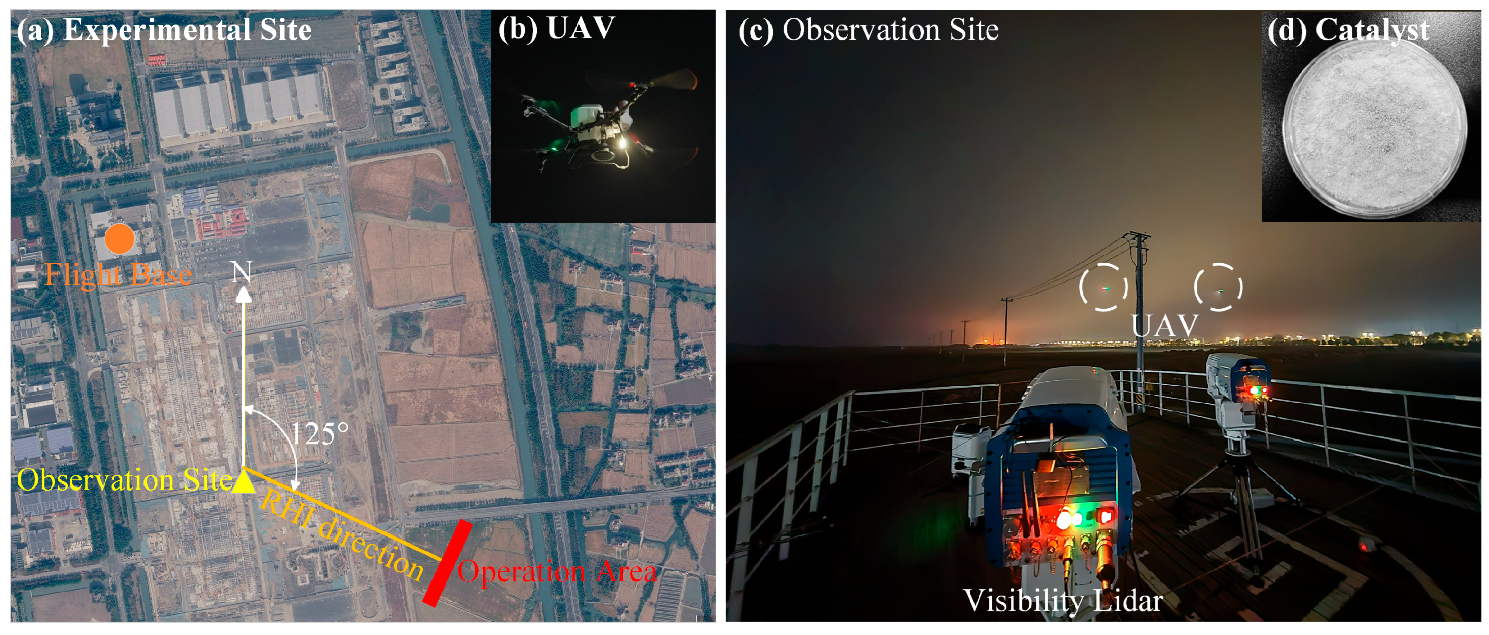
The field measurements were conducted at a site in Jinshan District, Shanghai, China (30°50′07.20″N, 121°20′59.92″E), which is approximately 3 m above mean sea level. The fog dispersal experiment was carried out near the UAV Base in Jinshan District, as shown in Figure 1a. This area is an important coastal area in southwest Shanghai, with a 23.3 km coastline. As shown in Figure 1b, the modified FlyCart 30 UAVs from SZ DJI Technology Co., Ltd.(Shenzhen, China), were deployed to spray the composite hygroscopic catalyst, with the operation area set to the southeast direction of the observation site. According to historical statistics from the local meteorological bureau, Jinshan District has an average of 23 fog days per year.

2.2. Hygroscopic Catalyst

The artificial fog dispersal catalyst used in this study is a new composite environmentally friendly functional material jointly developed by Chengdu University of Information Technology and the Weather Modification Center of China Meteorological Administration, as shown in Figure 1d. The catalyst takes environmentally friendly composite hygroscopic powder as the core component, supplemented by high-efficiency dispersants, stabilizers and molecular sieves. The proportions of each component are designed according to the characteristics of fog droplet size. After being uniformly released into the fog area by special spraying equipment on the UAV, it quickly combines with fog droplets to grow. Once liquid droplets of a certain size form, they begin to fall and trigger fog droplet coalescence. In a short time, the number, concentration and liquid water content of fog droplets decrease and the effective particle diameter increases, thus significantly improving visibility. The parameters of the hygroscopic catalyst are listed in

Table 1. The parameters of the hygroscopic catalyst.

Parameter	Value
Particle size range	8–9 μm
Main components	Hygroscopic material: sodium–calcium–magnesium composite salt Carrier material: fine mineral powder, plant cellulose, silicate micropowder, molecular sieve, etc. Stabilizer: inorganic nanopowder, synthetic alcohol ester, etc.
Active ingredient content	≥95%
Solubility	Dissolution rate ≤ 30 s (distilled water at 25 °C)
Acidity and alkalinity	pH ≈ 7–8 (after moisture absorption)
Density	2000–3000 kg·m−3
Applicable temperature	−20 °C~80 °C
Moisture absorption rate	0–5 min: 150 mg·min−1; 5–10 min: 90 mg·min−1; 10–30 min: 60 mg·min−1

.

2.3. Observation Equipment

The observation data in this experiment include automatic weather observation station (AWOS) data, coherent Doppler wind lidar data, visibility lidar data, etc. The automatic weather station is mainly used to obtain surface wind, temperature, humidity, pressure and visibility. The Doppler wind lidar adopts a vertical scanning mode to detect real-time background wind profiles. The main equipment used for operation effect evaluation in the artificial fog dispersal experiment is the TNL3 visibility lidar, produced by Wuxi Zhongke Optoelectronic Technology Co., Ltd (Wuxi, Jiangsu). The basic principle of this lidar observation system is that the laser emits laser pulse signals of a specific wavelength (1064 nm) into the atmosphere. Then pulse signals are scattered by water vapor molecules, atmospheric particles, etc., on the transmission path. The backscattered signals are received by the receiving telescope, converted into electrical signals by the detector in the receiving channel, collected by the signal acquisition unit, and finally inverted to calculate extinction coefficient and visibility. The extinction coefficient was retrieved using the Fernald method [19], and visibility is further inverted from the extinction coefficient according to the Koschmieder theory [20]. The detailed parameters are listed in

Table 2. The parameters of the visibility lidar.

Parameter	Value
Laser	Nd: YAG solid-state laser
Wave length	1064 nm
Single-pulse energy	100–400 μJ
Pulse repetition frequency	2–7 kHz
Telescope diameter	150 mm
Receiving field of view	1 mrad
Temporal resolution	8 s
Spatial resolution	15 m
Relative error	<50%, 50 m ≤ V ≤ 100 m <25%, 100 m < V ≤ 200 m <20%, >200 m
Maximum detection range	10 km
Scanning mode	DBS, PPI, RHI

. The visibility relative error ΔV/V ≤ 20%, for V > 200 m, where V denotes the true visibility and ΔV denotes the deviation between the lidar-retrieved visibility and the true value. The visibility lidar supports multiple scanning modes including Doppler Beam Swinging (DBS), PPI (Plan Position Indicator), range–height indicator (RHI) and other custom-defined modes. In this experiment, the visibility lidar was operated in RHI mode for the fog-dissipation effect evaluation. The RHI scanning was performed at a fixed azimuth angle of 125°. A complete RHI cycle consists of 10 elevation beams ranging from 17° to 26°. The acquisition time for each single radial beam was approximately 8 s with the full cycle being 80 s. This configuration ensured coverage of the target operation area and the downwind fog layer, enabling reliable spatial–temporal detection and quantitative assessment of the fog-dissipation effect.

2.4. Artificial Fog Dispersal Operation

According to the forecast of fog dispersal operation conditions, there would be a heavy-fog process in the early morning on 1 March 2025, with visibility below 500 m. This met the conditions for the artificial fog dispersal operation. Therefore, this period was finally selected to carry out the fog dispersal operation. The fog dispersal operation was carried out by the UAV spraying hygroscopic catalyst. The specific dispersal operation period is shown in

Table 3. Artificial fog dispersal operation period.

Number	Start Time (LT)	End Time (LT)
1	04:01	04:02
2	04:08	04:09
3	04:22	04:23
4	04:27	04:27
5	04:32	04:33
6	04:39	04:40

. The operation position takes the visibility lidar as the origin and the north direction as 0° for reference. The UAV flight trajectory is shown in Figure 1a. The UAV operation position was 230 m horizontally from the lidar and 120 m vertically above ground level. The catalyst was sprayed by the UAV flying back and forth along the tangential direction (125°), with a back-and-forth range of 30 m. For each seeding operation, the UAV carried 20 kg of hygroscopic catalyst, which was released completely during the flight. The typical spraying duration was approximately 40–50 s. Therefore, the average release rate was about 0.40–0.50 kg s⁻¹. The UAV flies at approximately 5 m/s along a 30 m round-trip.

2.5. Dispersal Effect Evaluation Method

Under heavy-fog conditions, single-point measurement results have deviations due to the strong scattering of fog droplets. During the fog dispersal operations, visibility was also affected by natural variability associated with evolving background meteorological conditions, as well as the measurement uncertainty due to dense fog conditions. To reduce these impacts on visibility evaluation results, a novel traversing window method based on the range–height indicator (RHI) mode of visibility lidar was proposed to quantitatively evaluate the spatial and temporal distribution of fog dispersal effects.

The method identifies local high-visibility regions within the expected operation-affected area and compares them with background reference windows to estimate the relative visibility enhancement. The procedure includes the following five steps:

Step 1: The raw lidar-bin visibility data are first projected into the horizontal-distance and height coordinate system and interpolated onto a 1 m grid for subsequent spatial analysis.

Step 2: Considering both the lidar range resolution and the operational scale of the fog-dissipation operation, a square moving window ($W$) with a size of 30 m × 30 m is then used to calculate the local mean visibility, and the window is located by the coordinates of its center point:

$$V_w\left(t\right)=\Sigma V_i\left(t\right)/N_w,i\in W$$

(1)

where $V_w\left(t\right)$ is the mean visibility of window $W$ at time $t$, $V_i\left(t\right)$ is the visibility value of the valid interpolated grid point inside the window, and $N_w$ is the number of valid data points in the window.

Due to the long scanning period, the time of the calculation result is selected as the beam detection time closest to the window center point to avoid visibility changes caused by time differences. Only windows with N_w > 8 were retained to avoid unreliable estimates from too few valid data points, which cannot reflect the real visibility level.

Step 3: A candidate search region is defined according to the UAV seeding height, the flight trajectory, and the prevailing wind direction during the operation. Because the released hygroscopic particles are expected to be transported downwind while settling downward, the search region is limited to the downwind area below the UAV seeding height. The moving window is then scanned within this predefined region to generate candidate windows for subsequent visibility ranking. This constraint is used to avoid selecting high-visibility windows that are unlikely to be directly associated with the UAV seeding plume.

Step 4: The mean visibility of each valid window is calculated and ranked. The window positions with higher visibility are screened out. Since the set traversal interval is small, there would be repeated calculations for the same or similar areas. Therefore, in the window screening process, it is required that the differences in both horizontal and vertical coordinates of the window centers are greater than 6 m.

Step 5: To reduce the influence of concurrent environmental variations, the region away from the expected direct seeding-influence area is selected as the background reference window. For each selected high-visibility window, the mean visibility of the contemporaneous background window is subtracted from that of the target window. The resulting difference is defined as the relative visibility enhancement associated with UAV seeding.

3. Results

3.1. Background Field Analysis

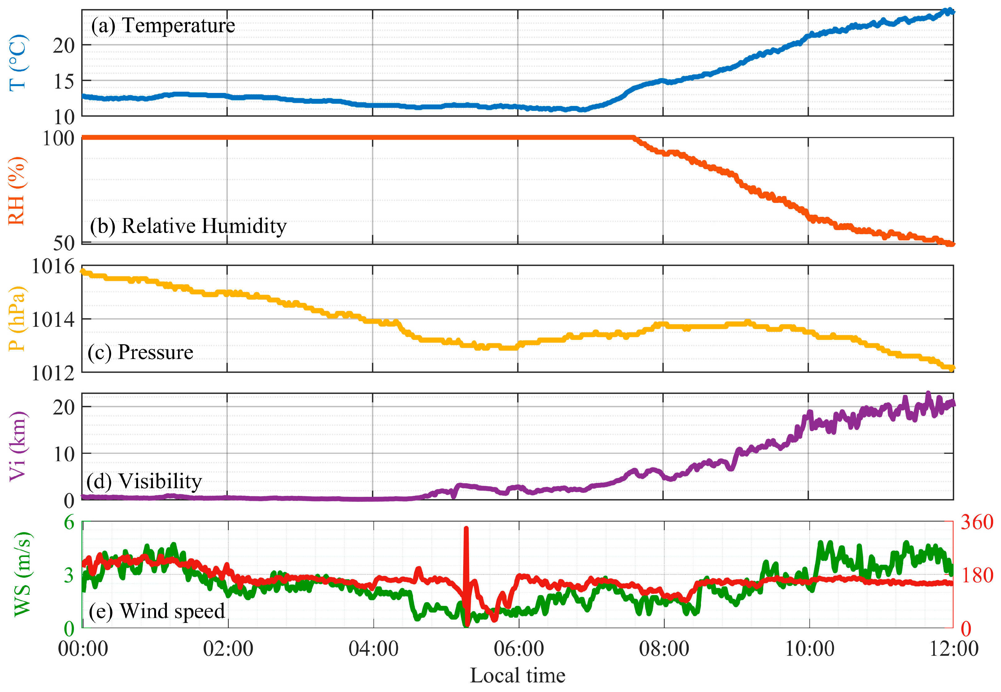
Figure 2 shows the time series of surface meteorological elements at the experimental site from 00:00 to 12:00 on 1 March 2025. The overall meteorological background field was stable in the early morning, providing typical conditions for the formation and maintenance of heavy fog and the development of the artificial fog dispersal operation. In terms of temperature, from 00:00 to 07:00, affected by nighttime radiative cooling, the temperature remained at a low level of 11–13 °C with very small fluctuations. As a result, a stable near-surface low-temperature layer was formed, which inhibited the vertical mixing and dissipation of the fog layer. After sunrise at 07:00, solar radiation increased, and the temperature rose linearly to about 23 °C at 12:00, as shown in Figure 2a. The relative humidity remained 100% saturated from 00:00 to 07:00, providing sufficient water vapor conditions for the maintenance of heavy fog. After 07:00, with the increase in temperature and fog dissipation, the relative humidity decreased rapidly to about 45% at 12:00, as shown in Figure 2b. The air pressure first decreased slowly from 1015.8 hPa at 00:00 to a minimum of 1013.0 hPa at 05:30, then rose slightly to 1013.9 hPa at 09:00, and finally declined slowly to below 1012 hPa at 12:00, as shown in Figure 2c. No abrupt pressure fluctuations were observed during the fog dispersal operation period (04:01–04:40), indicating a stable meteorological background and the absence of passing synoptic systems.

In terms of wind speed and direction, the near-surface wind speed generally remained at 2–4 m/s from 00:00 to 09:00, and the wind direction was stably south, as shown in Figure 2e. After 09:00, the wind speed gradually increased to 3–5 m/s, accelerating the diffusion and sedimentation of fog droplets. Although the wind direction shifted near the end of fog dissipation, the overall wind speed remained stable at 2 m/s. This stable wind field condition was the basis for selecting the southeast direction of the lidar as the operation area. This ensured that the sprayed hygroscopic catalyst could diffuse into the target fog area along the downwind direction.

Visibility was highly coupled with the above meteorological elements. It remained below 500 m from 00:00 to 05:00, reaching the heavy-fog level, which completely corresponded to 100% relative humidity. After 05:00, visibility began to rise slowly. After 08:00, visibility entered a rapid rising stage with the enhancement of solar radiation, and exceeded 20 km at 12:00. Overall, during the fog dispersal operation period (04:01–04:40), the temperature was stable at about 12 °C, the relative humidity was saturated, the wind speed was 1–2 m/s and the wind direction was stable. There were no violent fluctuations observed in the temporal variation in the air pressure. The stability of meteorological elements ensured that the catalyst could fully diffuse and play a hygroscopic growth role in the fog layer, providing ideal background conditions for the quantitative evaluation of artificial fog dispersal effect.

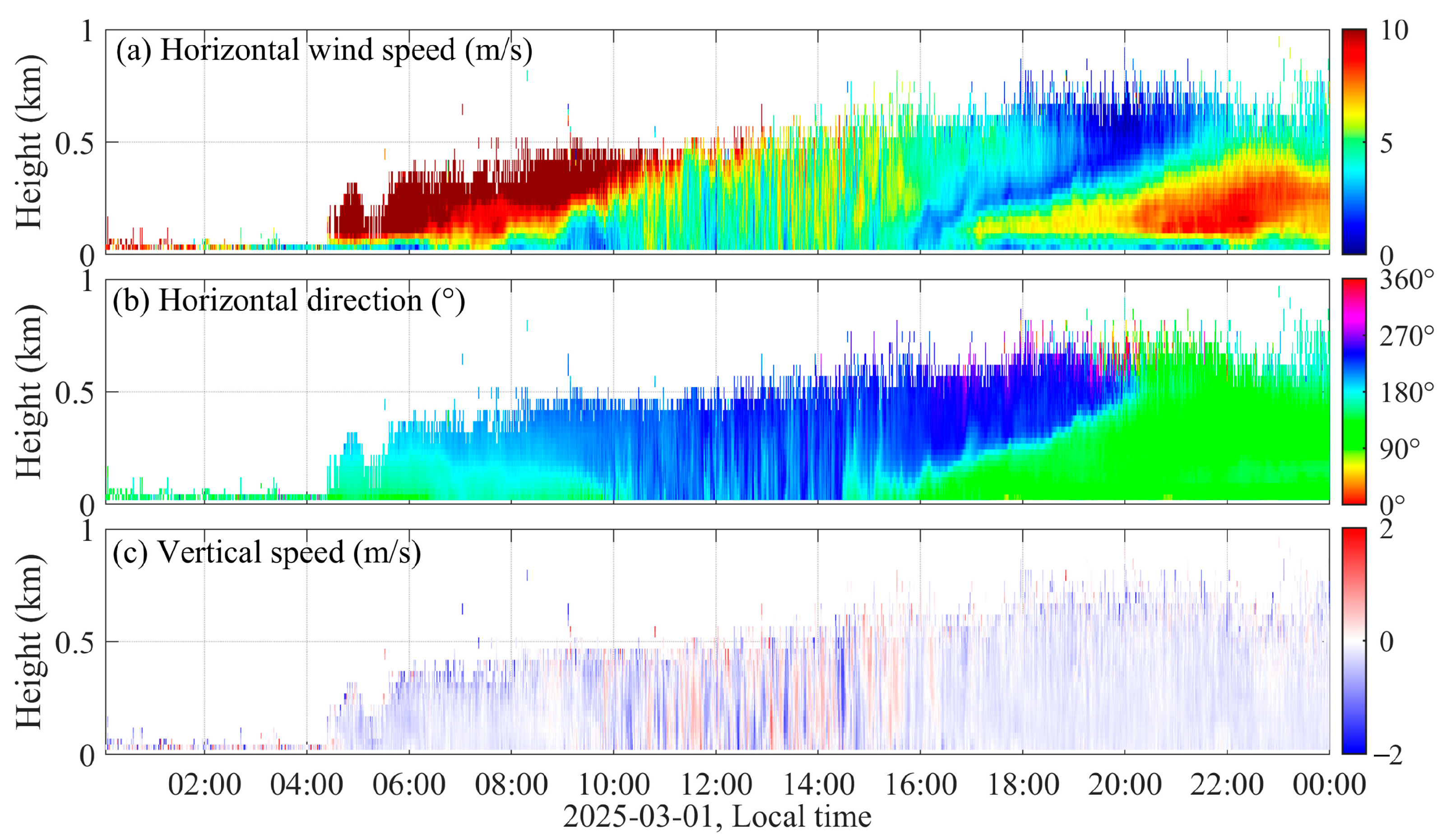
Figure 3 shows the spatiotemporal distribution of the wind profiles observed by the wind lidar at the experimental site on 1 March 2025. In terms of horizontal wind speed, from 00:00 to 04:30, no valid data was detected due to the strong attenuation of the laser by heavy fog. After 04:30, strong wind greater than 10 m/s was detected above 100 m, while the wind speed below 100 m was lower than 3 m/s. After 08:00, affected by solar radiation heating, the boundary layer gradually developed, and the wind speed increased significantly with height and time. The strong wind field accelerated the horizontal diffusion and vertical mixing of fog, becoming the main dynamic factor for the natural dissipation of fog. In terms of horizontal wind direction, the low altitude was dominated by southeast wind from 00:00 to 10:00. After 10:00–14:00, the wind direction gradually turned to southwest, and the boundary layer wind shear increased, indicating the transformation of local circulation. It switched to southeast wind after 16:00. The diurnal wind direction shift observed in this study reflected the transition of the land–sea breeze circulation. The dense fog in the early morning was formed by the combined effects of warm moist air advection over the cold underlying sea surface and enhanced nocturnal terrestrial longwave radiation cooling. In terms of vertical velocity, turbulence activity was weak at night. During the day, boundary layer turbulence activity increased, and the fluctuation amplitude of vertical velocity increased. This accelerated the mixing of fog droplets with upper dry air and promoted fog dissipation.

3.2. Artificial Dispersal Effect Evaluation

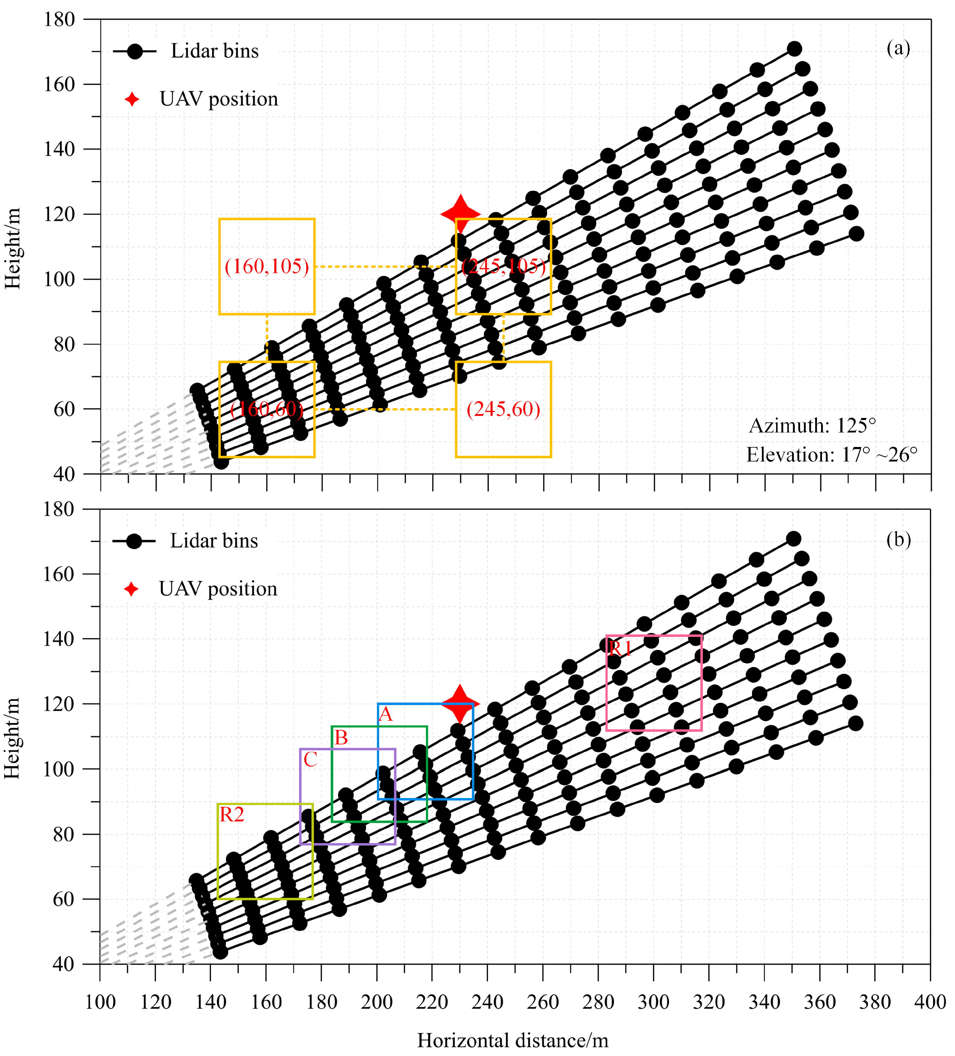
Based on the window-based visibility evaluation method described in Section 2.5, the RHI visibility data during the UAV fog-dissipation operations were analyzed to identify local high-visibility regions and to quantify the relative visibility enhancement after background correction. Figure 4a shows the detection range of the visibility lidar in RHI mode on 1 March 2025. The red star represents the UAV operation position with coordinates (230 m, 120 m). The radial beams of the lidar from bottom to top represent the elevation angle rising from 17° to 26° with 1° intervals. The black dots are the positions of lidar detection bins. Due to the detection blind area of the equipment, valid detection data starts at a radial distance of 150 m. The spatial resolution of the lidar is 15 m, and the detection range is up to 390 m, as shown in Figure 4a. The horizontal and vertical coordinates correspond to the horizontal distance and height of the lidar result positions.

Figure 4a shows a rectangular search region of 85 m × 45 m used to find the positions with better fog dispersal effect. The center point coordinates of the lower left window are (160 m, 60 m), and the center point coordinates of the upper right window are (245 m, 105 m). The window center was moved at 2 m intervals in both horizontal and vertical directions, producing 989 candidate windows.

As shown in Figure 4b, three positions with the most significant visibility improvement during the fog dispersal operation were selected, denoted as Window A, Window B, and Window C, with coordinates of (217 m, 105 m), (203 m, 99 m), and (189 m, 93 m), respectively. To compare variation characteristics of background fog, two windows were selected for comparison in the near field and far field of the lidar detection range, denoted as Window R1 and Window R2, with coordinates of (300 m, 125 m) and (160 m, 75 m), respectively.

Figure 5 shows the time series of visibility from the lidar for the five windows. It can be seen that the temporal variation characteristics of visibility at different positions are basically consistent, reflecting the dominant role of fog mass generation and dissipation in visibility changes during heavy fog. From 3:55 to 4:21 (covering the 1st and 2nd fog dispersal operations), affected by strong heavy fog, the visibility at the five positions was similar, ranging from 200 to 300 m. Due to the rapid replenishment of heavy fog in this stage, the lidar failed to capture obvious visibility improvement near the UAV operation range. The 3rd operation started at 4:22. At this time, the background fog concentration decreased, and the visibility at the five positions increased synchronously. By the end of the 6th operation, since the background fog replenishment became slower, the visibility in the operation-affected area was significantly higher than that in the background windows. At 4:42, the wind speed above about 100 m was greater than 10 m/s, and the heavy fog dissipated significantly. The overall visibility rose to more than 1000 m in a short time.

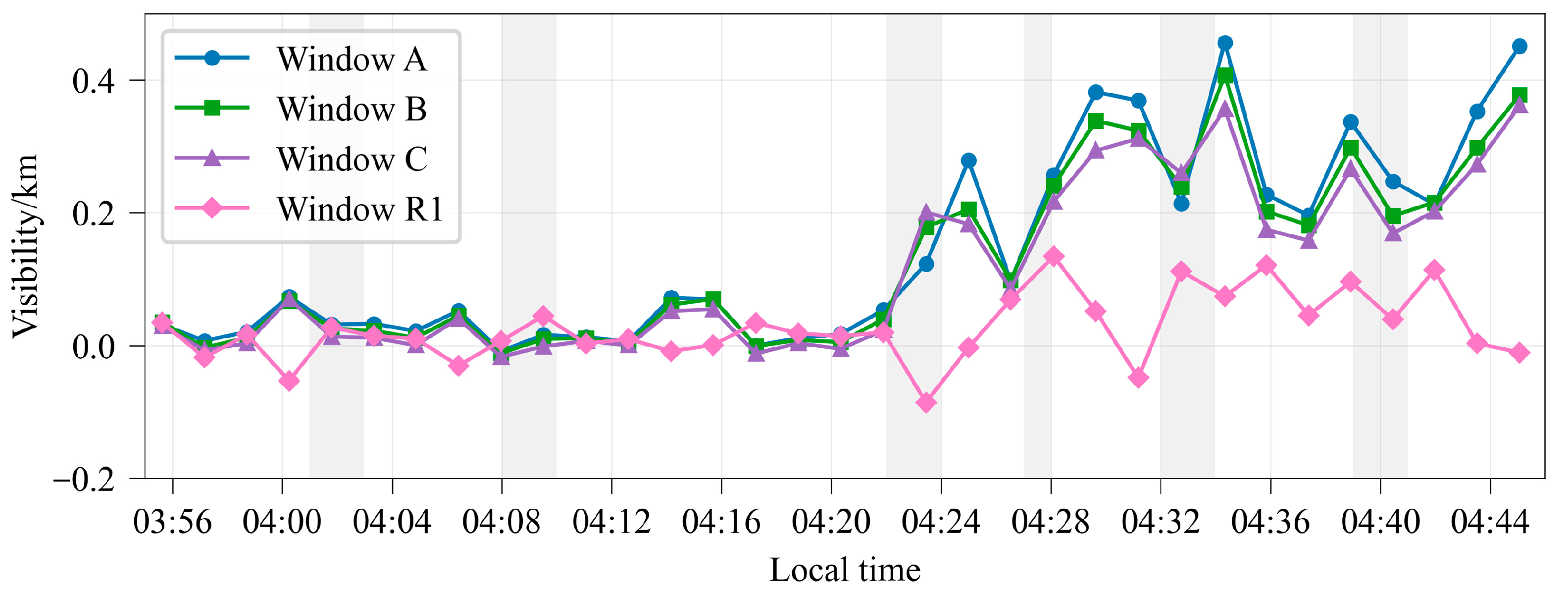
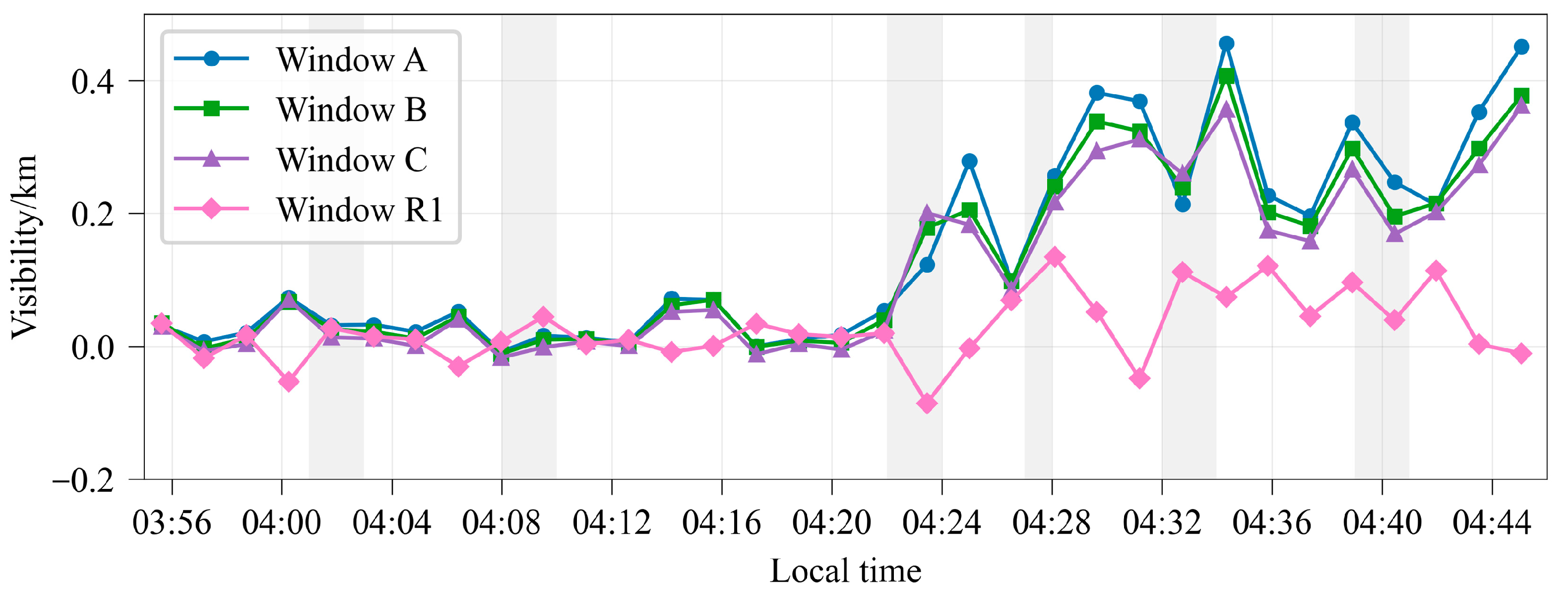
It can be seen that the difference between the far-field visibility and the near-field visibility was within ±100 m during the entire fog dispersal experiment, which reflects the rationality of selecting both as background references. From approximately 04:22 onward, the visibility in all windows showed an overall increasing trend, accompanied by short-term fluctuations, indicating that the fog field was affected by concurrent natural dissipation and replenishment. In particular, the enhanced wind above 100 m after approximately 04:30 may have promoted fog clearing through vertical mixing and dry-air entrainment. To reduce the influence of this natural evolution, Window R1 and Window R2 were selected as background reference windows outside the expected direct seeding-influence area. Their visibility variations represent the local background change during the same period. Since the visibility during the operation is the comprehensive performance of background fog change superimposed with catalyst influence, the near-field (Window R2) visibility was used as the background visibility to quantify the improvement. Specifically, the visibility values of Windows A, B, C and R1 were subtracted by the visibility value of the reference Window R2, respectively, and the results are shown in Figure 6.

The visibility improvement in the operation-affected area is consistent with the previous analysis of Figure 5. The first two operations had no obvious change due to the replenishment of strong heavy fog. Obvious improvement appeared from the 3rd operation. Visibility improvement effect had the following ranking: Window A > Window B > Window C. Its spatial distribution (Figure 4) is consistent with the catalyst movement trajectory; that is, the visibility improvement below the operation position and in the downwind direction is the most obvious. As the hygroscopicity of the catalyst decreases, the subsequent effect gradually weakens. In terms of the temporal variation in the difference, the peak in visibility improvement usually appears 2–3 min after the end of catalyst spraying. Subsequently, due to no continuous catalyst action, the improvement effect decreased significantly.

Window R1, located at a higher altitude, showed a stronger background visibility increase than Window R2 as a whole, which was consistent with its greater exposure to upper-level ventilation. The maximum improvement of 456 m at 04:34 was obtained relative to R2, whereas the enhancement relative to R1 at the same time was 382 m. When R1 was used as the background reference, the maximum relative improvement was 417 m at 04:31. Therefore, by subtracting the results from the background Windows R1 and R2, the influence of weather conditions can be excluded to a certain extent, reflecting the effect of the catalyst.

4. Discussion

It should be noted that multiple scattering may introduce systematic bias into the retrieved extinction coefficient and visibility under dense fog conditions. Therefore, window-averaged visibility values were adopted, rather than individual beam measurements, to reduce the influence of such bias on the evaluation. Nevertheless, without synchronous vertical comparison measurements from auxiliary instruments, spatially heterogeneous retrieval errors of the visibility lidar cannot be fully isolated from the seeding-induced visibility improvement. Thus, potential bias introduced into the visibility evaluation remains non-negligible. During the entire observation period, the lidar-derived visibility was generally greater than 200 m. Therefore, the upper limit of the relative uncertainty can be taken as 20%. Since the measurement errors from different beams within each averaging window can be regarded as independent, the relative uncertainty of the window-averaged visibility is expected to be lower than 20%.

The visibility lidar observations indicate a localized visibility response in the region expected to be affected by the UAV operation. Comparison with both reference windows showed that the target windows exhibited an additional local visibility enhancement in the operation-relevant area. The differing enhancement magnitudes obtained with R1 and R2 demonstrate the sensitivity of the result to the vertical background state. The window-based comparison reduces the influence of the common temporal visibility trend, but it cannot completely remove the effects of spatially heterogeneous meteorological evolution.

Thus, the reported enhancement should be interpreted as a local visibility anomaly associated with UAV seeding under naturally evolving fog conditions.

The location and timing of the enhanced-visibility region are compatible with the expected downwind transport of hygroscopic particles below the UAV seeding height. Based on the catalyst properties and warm fog seeding theory, hygroscopic growth, collision-coalescence, and sedimentation may provide plausible explanations for this response. However, no direct measurements of droplet size distribution, liquid water content, droplet number concentration, or catalyst concentration were available. Future experiments should combine multi-wavelength lidar with in situ microphysical measurements and, where feasible, tracer or catalyst-concentration observations to establish the link between the seeding material, microphysical changes, and visibility response.

5. Conclusions

This study developed a traversing window method using RHI visibility lidar observations to evaluate the local visibility response during UAV hygroscopic seeding of coastal warm fog. The method identifies high-visibility windows within the operation-relevant region and quantifies their relative enhancement through comparison with concurrent background reference windows. This experiment was a typical coastal radiation fog process. The meteorological background field was stable during the fog dispersal operation period. The near-surface wind was weak and the wind direction was constant southeast. The relatively stable background conditions ensured that the catalyst fully stayed at the target height of 90–120 m and coalesced with fog droplets. Through background window subtraction, the interference of the natural change in fog and measurement uncertainty is suppressed. The experimental results show that the new composite hygroscopic catalyst has a dispersal effect on coastal warm fog, and its effect is closely related to the background fog concentration. The catalyst effect was masked by the rapid replenishment of fog masses in the strong heavy-fog stage, and became prominent when the background fog concentration decreased. The best dispersal effect was observed below the operation position and in the downwind direction. The traversing window method effectively overcomes the contingency and one-sidedness of traditional single-point evaluation, and can identify the optimal area of fog dispersal effect and quantify its intensity.

This study still has certain limitations. The maximum relative visibility enhancement reached 456 m compared with R2 and 417 m compared with R1. These results support a local visibility enhancement associated with UAV hygroscopic seeding. However, because the experiment was conducted during an evolving natural fog-dissipation process, the contribution of meteorological changes cannot be completely excluded, and the systematic uncertainty associated with dense fog conditions still remains. Only a single field fog dispersal experiment was analyzed, and the sample size is limited. It is hard to fully reflect the fog dispersal effect under different meteorological conditions. Only the detection data from a single azimuth of lidar RHI mode was used for evaluation, lacking a complete description of the three-dimensional fog dispersal effect in the operation area. The influence of parameters such as catalyst dosage, spraying height and flight speed on the fog dispersal effect was not systematically quantified. The current observations can quantify visibility variation but cannot directly verify the microphysical pathway. Additional in situ measurements or multi-wavelength remote sensing observations would considerably strengthen the interpretation of the dispersal mechanism. In the future, we will further increase the number of field experiment samples under different fog and meteorological conditions, carry out multi-parameter comparative experiments, realize three-dimensional effect evaluation by combining lidar PPI and RHI multi-mode detection, optimize catalyst formulation and UAV spraying strategy, and provide solid technical support for the operational application of artificial fog dispersal in key areas such as the Yangtze River Delta coastal port group and airports.

References

- Gultepe, I.; Tardif, R.; Michaelides, S.C.; Cermak, J.; Bott, A.; Bendix, J.; Müller, M.D.; Pagowski, M.; Hansen, B.; Ellrod, G.; et al. Fog Research: A Review of Past Achievements and Future Perspectives. Pure Appl. Geophys. 2007, 164, 1121–1159. [Google Scholar] [CrossRef] [Scilit]
- Park, M.-G.; Kang, H.-S.; Kim, Y.-J. A Study on the Effectiveness of SCD Seeding Fog Dissipation Mechanism Using LiDAR Sensor. Fluids 2023, 8, 185. [Google Scholar] [CrossRef] [Scilit]
- Vonnegut, B. Experiments with Silver Iodide Smokes in the Natural Atmosphere. Bull. Am. Meteorol. Soc. 1950, 31, 151–157. [Google Scholar] [CrossRef] [Scilit]
- Beckwith, W.B. Supercooled fog dispersal for airport operations. Bull. Am. Meteorol. Soc. 1965, 46, 323–327. [Google Scholar] [CrossRef] [Scilit]
- Lu, Z.; Sun, B.; An, Y. A Low-Level Air Heating Method to Dissipate Dense Fog on Highways. J. Transp. Eng. Part B Pavements 2025, 4, 151. [Google Scholar] [CrossRef] [Scilit]
- Kumai, M. Formation of Ice Crystals and Dissipation of Supercooled Fog by Artificial Nucleation, and Variations of Crystal Habit at Early Growth Stages. J. Appl. Meteorol. Climatol. 1982, 21, 579–587. [Google Scholar] [CrossRef] [Scilit] [PubMed]
- Koracin, D.; Dorman, C.E.; Lewis, J.M.; Hudson, J.G.; Wilcox, E.M.; Torregrosa, A.A. Marine Fog: A Review. Atmos. Res. 2014, 143, 142–175. [Google Scholar] [CrossRef] [Scilit]
- Weinstein, A.I. Fog dispersal-A technology assessment. J. Aircr. 1977, 14, 38–43. [Google Scholar] [CrossRef] [Scilit] [PubMed]
- Liu, C.; Tian, Z.; Zhao, Y.; Zeng, X. Review and prospect of fog elimination technology based on acoustic condensation. In Proceedings of IOP Conference Series: Earth and Environmental Science; IOP Publishing: Bristol, UK, 2020; Volume 514, p. 032011. [Google Scholar] [CrossRef] [Scilit]
- Kunkel, B.A. A modern thermo-kinetic warm fog dispersal system for commercial airports. J. Appl. Meteorol. Climatol. 1979, 18, 794–803. [Google Scholar] [CrossRef] [Scilit] [PubMed]
- Silverman, B.A.; Kunkel, B.A. A numerical model of warm fog dissipation by hygroscopic particle seeding. J. Appl. Meteorol. Climatol. 1970, 9, 627–633. [Google Scholar] [CrossRef] [Scilit] [PubMed]
- Alekseeva, A.; Davidov, V.; Ivanov, V.; Palei, A.; Pisanko, Y.; Savchenko, A.; Vasilyeva, M.; Vasilev, A.; Zinkina, M. Warm Fog Artificial Dispersion, Preliminary Results. J. Atmos. Sci. Res. 2025, 8, 51–64. [Google Scholar] [CrossRef] [Scilit]
- Khain, A.; Pinsky, M.; Gavze, E.; Ronen, A.; Elisha, S.; Shoshanim, O.; Khain, P. Warm Fog Elimination by Seeding with Salty Drops: Experiments and Theory. J. Weather Modif. 2024, 55. [Google Scholar] [CrossRef]
- Cheng, L.; Jia, Y.-H.; Li, F.-F.; Qiu, J. Cloud chamber experimental study for acoustic fog elimination technology. Appl. Acoust. 2024, 219, 109885. [Google Scholar] [CrossRef] [Scilit]
- Alekseeva, A.; Davidov, V.; Paley, A.; Pisanko, Y.; Schelkalin, A.; Zinkina, M. On Prevention and Treatment of Warm Fog on Highways with the Help of Spatially Inhomogeneous Electric Field. Prev. Treat. Nat. Disasters 2025, 4, 64–76. [Google Scholar] [CrossRef]
- Khalid, S.; Gupta, S.K.; Chakkaravarthy, M.; Prakash, D.; Agrawal, A.; Nishad, D.K. AI-Optimized UAV Swarm System for Radiation Fog Dispersal and Runway Visibility Enhancement at Airport. Int. J. Aeronaut. Space Sci. 2025, 27, 2423–2450. [Google Scholar] [CrossRef] [Scilit]
- Khalid, S.; Chakkaravarthy, M.; Gupta, S.K.; Prakash, D.; Agrawal, A.; Nishad, D.K. A conceptual framework for developing an AI-powered UAV system for effective fog management at airports. SPAST Rep. 2025, 1. Available online: https://spast.org/ojspath/article/view/5199 (accessed on 1 August 2026).
- DeFelice, T.P.; Axisa, D. Modern and Prospective Technologies for Weather Modification Activities: Developing a Framework for Integrating Autonomous Unmanned Aircraft Systems. Atmos. Res. 2017, 193, 173–183. [Google Scholar] [CrossRef] [Scilit]
- Fernald, F.G. Analysis of atmospheric lidar observations: Some comments. Appl. Opt. 1984, 23, 652–653. [Google Scholar] [CrossRef] [Scilit] [PubMed]
- Katsev, I.; Zege, E. The modern theory of black object visibility and meteorological visibility range. Atmos. Environ. 1994, 28, 763–767. [Google Scholar] [CrossRef] [Scilit]