Controlled Evaluation of Sentinel-2 Annual Compositing Strategies for Deep Learning-Based Mangrove Mapping in China

Highlights

What are the main findings?

• Sentinel-2 annual compositing rules produced substantial differences in mangrove mapping accuracy and in the balance between omission and commission errors under a common deep learning framework.
• The median annual composite provided the most balanced accuracy among the tested compositing rules for 10 m mangrove mapping in China.

What are the implications of the main findings?

• Annual image compositing is an important source of variation in deep learning-based mangrove mapping and should be evaluated explicitly rather than treated as a routine preprocessing step.
• Median compositing offers a practical and stable input strategy for Sentinel-2-based national-scale mangrove monitoring under the coastal conditions examined in this study.

Abstract

Accurate national-scale mangrove mapping remains challenging because mangroves occur in narrow intertidal belts affected by tidal variation, residual clouds, water background effects, and spectral confusion with adjacent vegetation. This study evaluated five Sentinel-2 annual compositing rules for 10 m mangrove mapping in China: MAX-KNDVI, MAX-EVI, a negative-NDWI-based composite, MAX-MFI, and Median compositing. A single shared ResNet-34 U-Net model was trained using pooled patches from the five rule-specific composites and was then applied separately to each composite. Labelled sample locations, validation data, probability threshold, and post-processing settings were kept consistent to focus the comparison on the compositing rule. Using 695 labelled patch locations and 10,354 spatially independent validation points from 29 coastal regions, the Median-based output achieved the most balanced performance among the tested rules, with an overall accuracy of 90.1% and a Kappa coefficient of 0.801. Compared with GMW v3.0, HGMF_2020, and LREIS_v2_2020, the Median-based output showed higher agreement with the independent validation samples and fewer omissions in selected fragmented coastal zones. Applying the Median configuration to annual Sentinel-2 composites from 2019 to 2023 indicated an increase in mapped mangrove area in China from 22,731.76 ha to 24,631.62 ha. These results show that annual compositing-rule selection is an important source of performance variation in Sentinel-2 deep learning-based mangrove mapping and should be considered explicitly in national-scale coastal wetland monitoring.

1. Introduction

Mangrove forests are highly valuable coastal wetland ecosystems that support biodiversity and store large amounts of blue carbon [1]. They also provide important coastal protection services by reducing shoreline erosion, attenuating waves, and buffering coastal hazards [2,3]. Reliable information on mangrove distribution is therefore essential for conservation planning, restoration assessment, and coastal wetland management. Accurate large-scale mangrove mapping remains challenging because mangroves often occur as narrow and fragmented intertidal belts where tidal variation, mixed pixels, and spectral confusion with adjacent land-cover types can reduce classification consistency [4]. These difficulties are further complicated by the spectral variability of mangrove canopies and surrounding coastal backgrounds [5,6]. For satellite-based national-scale mapping, a stable and representative annual image composite is therefore required before reliable mangrove delineation can be achieved.

These challenges are particularly evident along the coast of China. Chinese mangroves are mainly distributed in subtropical and tropical coastal regions, where they often occur as narrow belts, small patches, or restored stands along estuaries, bays, aquaculture ponds, tidal flats, and modified shorelines [7]. Long-term monitoring studies have shown that mangrove loss and recovery in China have been strongly shaped by conservation, restoration, and coastal land-use change [8]. Remote sensing studies have also reported that mangroves can be difficult to separate from salt marshes and other adjacent coastal land-cover types [9,10]. Such classification challenges are especially pronounced for fragmented shoreline patches and recently restored stands, and their severity varies among coastal environments. Residual clouds, haze, tidal exposure, water-background effects, and mixed pixels further reduce the temporal stability and spectral separability of mangrove signals [4,5,6,9]. For national-scale Sentinel-2 mapping, the methodological challenge is therefore not only classifier design, but also the construction of annual input images that consistently represent mangrove and non-mangrove coastal surfaces.

Annual image compositing is widely used to reduce the influence of clouds, atmospheric contamination, and short-term surface variability in optical remote sensing time series [11]. For dense Sentinel-2 and Landsat observations, compositing algorithms can substantially affect the reflectance values retained in the final image and, consequently, the information provided to land-cover classifiers [12,13]. Quality-mosaic approaches select one observation per pixel according to a defined quality band, so residual haze, sun glint, turbidity, or unusual tidal conditions may also be retained [11,12,13]. Median compositing can reduce these short-lived extremes but may attenuate temporally specific phenological or hydrological signals [12,13]. In addition, KNDVI-, EVI-, MFI-, and negative-NDWI-based rules emphasize different spectral characteristics [14,15,16,17], potentially affecting the contrast between mangroves and surrounding coastal classes. Mangrove-specific spectral indices, such as the mangrove vegetation index (MVI), have also been developed to enhance the spectral discrimination of mangrove vegetation [18]. Such compositing-related differences can alter the spectral-spatial characteristics of the resulting annual image inputs and may subsequently influence deep learning-based mangrove segmentation [19]. However, previous regional and national studies differed in sensors, classifiers, samples, compositing strategies, and geographic settings, making it difficult to isolate the effect of the compositing rule itself. A controlled comparison under a consistent segmentation and validation framework is therefore necessary.

Compositing rules do more than produce visually different annual images. They determine which observations are selected or summarized for each pixel and can therefore alter the spectral-spatial patterns learned by downstream classification models.

Deep learning models have shown strong potential for remote sensing image segmentation because they can learn nonlinear spectral-spatial features from complex image data [19]. Recent mangrove mapping studies have also demonstrated the ability of deep learning models to delineate mangrove boundaries and fragmented patches at high spatial resolution [19]. Nevertheless, model performance remains constrained by the quality, stability, and representativeness of the input image composites. A strong segmentation model cannot fully compensate for residual cloud contamination, tidal artefacts, water-background effects, or inconsistent spectral signals introduced during annual compositing. Deep learning-based mangrove mapping should hence be evaluated together with the compositing strategy used to construct the annual input image. Without such control, it is difficult to determine whether accuracy differences arise mainly from the classifier, the input composite, or their interaction.

Several global and regional mangrove products have demonstrated the feasibility of large-scale mangrove monitoring at 10 m or finer spatial resolution. Global Mangrove Watch version 3.0 provides a long-term global mangrove extent dataset from 1996 to 2020 [20]. LREIS_GLOBALMANGROVE_v2 provides 10 m global mangrove classification products for 2018–2020 [21]. HGMF_2020 maps global mangrove forest distribution at 10 m resolution [22]. Despite these advances, local omissions and boundary inconsistencies may still occur along China’s fragmented and tidally dynamic shorelines, particularly around aquaculture ponds, narrow mangrove belts, and recently restored stands. Multi-source approaches that combine optical imagery, synthetic aperture radar, and multi-resolution features can improve mangrove classification under complex coastal conditions [23,24,25]. However, these approaches often require additional data sources, more preprocessing steps, and higher computational cost. Sentinel-2 annual compositing remains an operationally attractive strategy for national-scale mangrove monitoring, but the effects of different compositing rules have not been sufficiently tested under a controlled deep learning framework.

To address this gap, this study evaluated five rule-specific Sentinel-2 annual composites for 10 m mangrove mapping in China. The compositing rule was treated as the main experimental variable, whereas the ResNet-34 U-Net architecture, labelled sample locations, validation data, probability threshold, and post-processing settings were kept consistent. The objectives were to (1) compare maximum kernel normalized difference vegetation index-based composite (MAX-KNDVI), maximum enhanced vegetation index (MAX-EVI), negative normalized difference water index (negative-NDWI), maximum mangrove forest index (MAX-MFI), and Median compositing for deep learning-based mangrove mapping; (2) evaluate the selected output against GMW v3.0, HGMF_2020, and LREIS_v2_2020 using spatially independent validation samples; and (3) apply the selected configuration to map annual mangrove distribution in China from 2019 to 2023 and summarize mapped area changes. By isolating the compositing rule within a shared segmentation framework, this study clarifies how annual image representation affects Sentinel-2 deep learning-based mangrove mapping and provides practical guidance for national-scale coastal wetland monitoring.

2. Materials and Methods

2.1. Coastal Study Domain, Reference Samples, and Ancillary Datasets

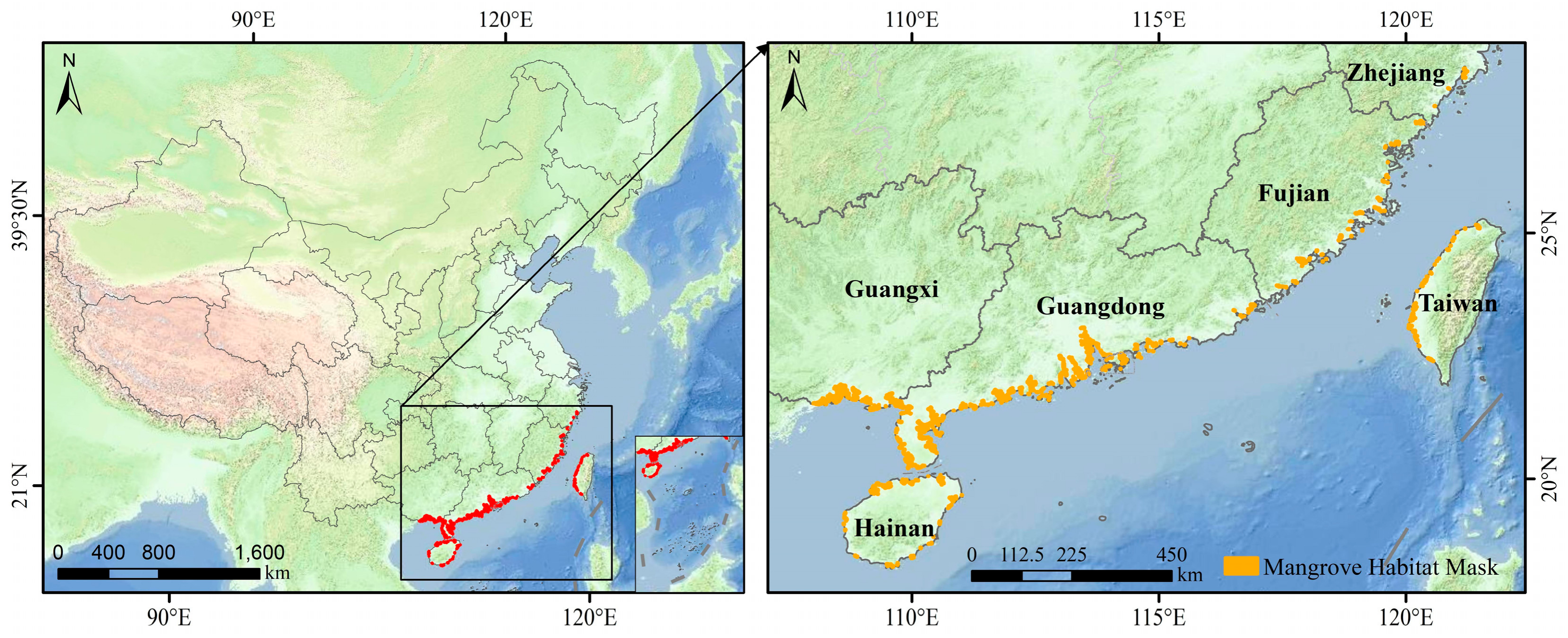
Mangrove forests in China are mainly distributed along the subtropical and tropical southeastern coastline, including Hainan, Guangdong, Guangxi, Fujian, Zhejiang, and Taiwan [7]. These regions include estuaries, bays, deltas, lagoons, tidal flats, aquaculture ponds, and highly modified shorelines, which together create complex coastal backgrounds for mangrove mapping [8]. In this study, mangrove forests refer to the woody mangrove vegetation component of coastal mangrove wetland ecosystems. The coastal study domain is shown in Figure 1.

To define the modelling domain, existing mangrove products and field-surveyed mangrove features were merged to form an envelope of known mangrove occurrence. An isotropic 10 km buffer was then applied to this envelope to include representative coastal background classes that are spectrally or spatially confusable with mangroves, including tidal flats, aquaculture ponds, coastal evergreen vegetation, water bodies, and modified shorelines. The 10 km distance was selected as a practical compromise to retain representative coastal background variability while avoiding extensive inland and open-ocean areas unrelated to mangrove mapping. The buffer was used to define the modelling domain as distinct from an ecological influence distance of mangroves. The buffered domain was clipped by coastal administrative boundaries to retain coastal land–water transition zones while reducing open-ocean areas unlikely to contain mangroves. Buffering and area calculations were performed in projected coordinate systems to preserve distance and area fidelity.

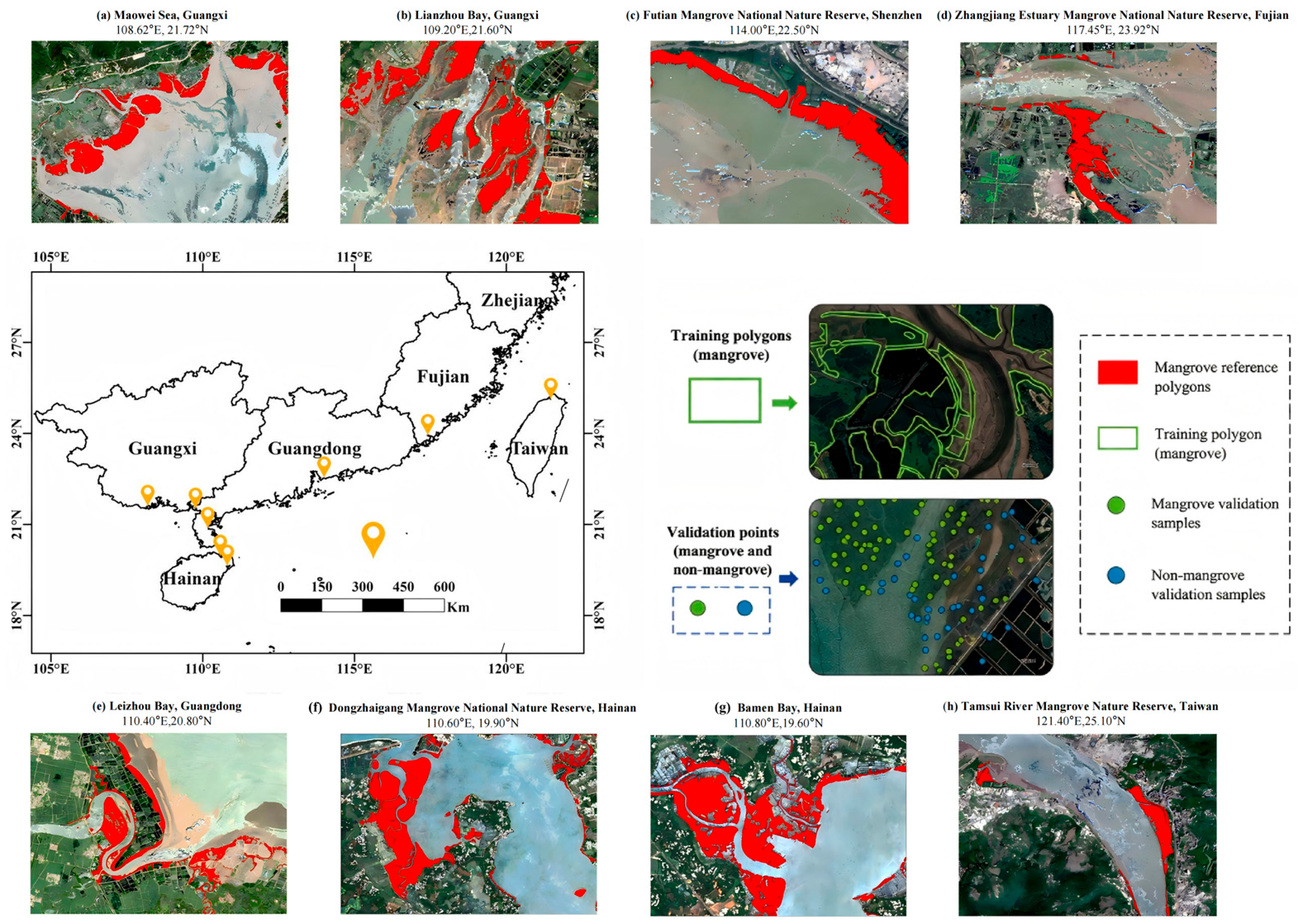
Field reference data were collected from 34 coastal survey regions (Figure 2). A detailed survey of mangrove distribution on Hainan Island had been conducted before this study [26]. Additional field surveys were conducted between February and June 2021 in parts of Hainan, Guangxi, Guangdong, and Fujian. Handheld GPS devices and high-resolution Google Earth imagery were used to support field positioning and reference interpretation. Training samples were collected from five survey regions, yielding 695 labelled patch locations. Each input patch contained 12 Sentinel-2 spectral bands and had a size of 128 × 128 pixels. At the 10 m spatial resolution, each patch represented an area of approximately 1.28 km × 1.28 km, providing sufficient spatial context to capture fragmented mangrove patches and their surrounding coastal backgrounds while maintaining computational efficiency. External validation samples were obtained from the remaining 29 survey regions, which were not used for model training. A total of 10,354 reference points were used for external validation, including 5208 mangrove points and 5146 non-mangrove points. The separation between the training and validation survey regions was used to reduce the risk of inflated accuracy caused by spatially proximate samples. Taiwan was included in the mapping and area summaries but was not used for field sampling or model training; its results were therefore interpreted as an external application area instead of a field-validated region. Three existing mangrove products were used for product-level comparison. Global Mangrove Watch version 3.0 provides global mangrove extent information through 2020 [20]. LREIS_GLOBALMANGROVE_v2 provides 10 m global mangrove classification products for 2018–2020 [21]. HGMF_2020 provides a 10 m global mangrove forest map for 2020 [22]. Because the field reference data mainly corresponded to 2020, the 2020 layers of these products were used for external comparison.

Ancillary climate and land-use datasets were used only for exploratory association analysis and were not used for model training. Annual maximum, minimum, and mean land surface temperature were derived from the MOD11A1.061 Terra LST product [27]. Annual total precipitation was derived from the CHIRPS daily precipitation dataset [28]. Annual cropland and built-up areas were summarized from the Esri 10 m annual land-use dataset [29].

2.2. Sentinel-2 Annual Compositing Under Coastal Cloud and Water-Background Effects

Sentinel-2 surface reflectance imagery from 1 January 2019 to 31 December 2023 was obtained from the COPERNICUS/S2_SR_HARMONIZED collection in Google Earth Engine [30]. Images with CLOUD_COVERAGE_ASSESSMENT values greater than 20% were excluded before annual compositing. Cloud- and cirrus-contaminated pixels were masked using the QA60 band, in which bits 10 and 11 indicate opaque clouds and cirrus clouds, respectively [31]. This filtering and masking procedure was applied consistently to all compositing rules to maintain comparability among the rule-specific annual composites.

Twelve Sentinel-2 spectral bands were retained for classification: B1, B2, B3, B4, B5, B6, B7, B8, B8A, B9, B11, and B12. All selected bands were prepared on a common grid and exported at 10 m spatial resolution for patch-based segmentation. The spectral indices described below were used only as quality bands for selecting annual observations during compositing. They were not appended as additional input channels to the deep learning model.

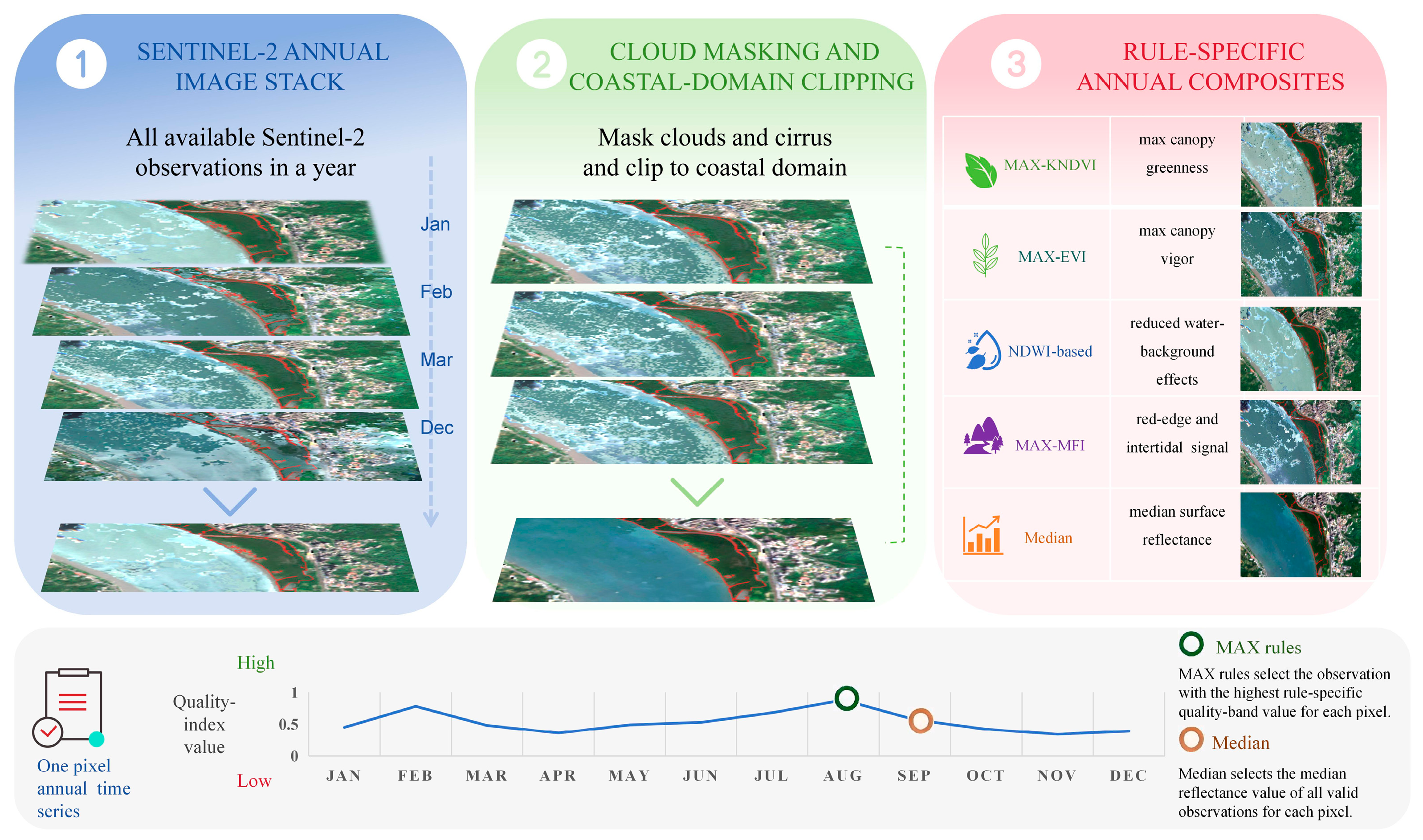
Five annual compositing rules were designed to represent different annual surface conditions relevant to mangrove mapping. Four rule-specific composites were generated using the qualityMosaic() function in Google Earth Engine. For each pixel, qualityMosaic() selects the observation with the highest value of a user-defined quality band, and the corresponding Sentinel-2 spectral bands from that same observation are retained in the output composite. KNDVI [16], an EVI-based quality band [17], negative NDWI [14], and MFI [15] were used to generate the MAX-KNDVI, MAX-EVI, negative-NDWI-based, and MAX-MFI composites, respectively. The workflow used to generate the five rule-specific annual composites is shown in Figure 3.

KNDVI was used to emphasize annual maximum canopy greenness [16]. The EVI-based quality band was used to rank observations according to vegetation vigour and vegetation-background contrast [17]. MFI was used to enhance red-edge and intertidal spectral characteristics associated with mangrove environments [15]. For the negative-NDWI-based rule, negative NDWI was used as the quality band so that the selected observation corresponded to the lowest NDWI value within the annual image stack [14]. This design was intended to reduce the influence of water-background and tidal-water conditions in coastal pixels.

An annual Median composite was also generated from all valid observations. Median compositing summarized the central tendency of valid annual reflectance observations for each spectral band and reduced the influence of short-lived spectral extremes caused by residual clouds, haze, water-surface glint, turbidity, or unusual tidal states. The five rule-specific annual composites were then evaluated under the same segmentation framework to determine how annual compositing-rule selection affected mangrove mapping performance. The quality bands and compositing rules are summarized in

Table 1. Quality bands and annual compositing rules used in this study.

Rule	Quality Band/Selection Rule	Formula or Rule	Intended Compositing Signal
MAX-KNDVI	KNDVI	$\begin{array}{rr}& Q_{\mathrm{KNDVI}}=\tanh \left({\mathrm{NDVI}}^2\right), \mathrm{NDVI}=\left({\rho }_{\mathrm{NIR}}-{\rho }_{\mathrm{Red}}\right)/\left({\rho }_{\mathrm{NIR}}+{\rho }_{\mathrm{Red}}\right)\end{array}$	Maximum canopy greenness
MAX-EVI	EVI-based quality band	$\mathrm{E}\mathrm{V}\mathrm{I}=2.5\times {\displaystyle \frac{\mathrm{N}\mathrm{I}\mathrm{R}-\mathrm{R}\mathrm{e}\mathrm{d}}{\mathrm{N}\mathrm{I}\mathrm{R}+6\mathrm{R}\mathrm{e}\mathrm{d}-7.5\mathrm{B}\mathrm{l}\mathrm{u}\mathrm{e}+1}}$	Relative canopy vigour/vegetation contrast
NDWI-based	Negative NDWI	$\begin{array}{rr}& Q_{\mathrm{NDWI}}=-\mathrm{NDWI}, \mathrm{NDWI}={\displaystyle \frac{\mathrm{G}\mathrm{r}\mathrm{e}\mathrm{e}\mathrm{n}-\mathrm{N}\mathrm{I}\mathrm{R}}{\mathrm{G}\mathrm{r}\mathrm{e}\mathrm{e}\mathrm{n}+\mathrm{N}\mathrm{I}\mathrm{R}}}\end{array}$	Reduced water-background and tidal-water effects
MAX-MFI	MFI	$\begin{array}{rr}& Q_{\mathrm{MFI}}={\displaystyle \frac{\left({\rho }_{705}-{\rho }_{705}^{\mathrm{b}}\right)+\left({\rho }_{740}-{\rho }_{740}^{\mathrm{b}}\right)-\left({\rho }_{783}-{\rho }_{783}^{\mathrm{b}}\right)+\left({\rho }_{865}-{\rho }_{865}^{\mathrm{b}}\right)}{4}}\end{array}$	Red-edge and intertidal mangrove signal
Median	Median reflectance	Median value of each spectral band across valid annual observations	Temporally stable annual surface condition

Note: $\rho$ denotes Sentinel-2 surface reflectance. For MFI, ${\rho }^{\mathrm{b}}$ lambda is the baseline reflectance between 665 and 2190 nm. The EVI-based quality band follows the GEE implementation used in this study. Quality bands were used only for annual compositing; the exported model inputs were the selected 12 Sentinel-2 spectral bands.

.

2.3. Common Segmentation Framework for Rule-Specific Mangrove Segmentation

Mangrove mapping was formulated as a binary semantic segmentation task. MR_DLM_2020 was designed as a common segmentation framework for evaluating the influence of Sentinel-2 annual compositing rules on mangrove forest mapping. In this framework, the rule-specific annual composite was the factor varied during inference, whereas the network architecture, labelled sample locations, validation design, training strategy, probability threshold, and post-processing settings were kept consistent.

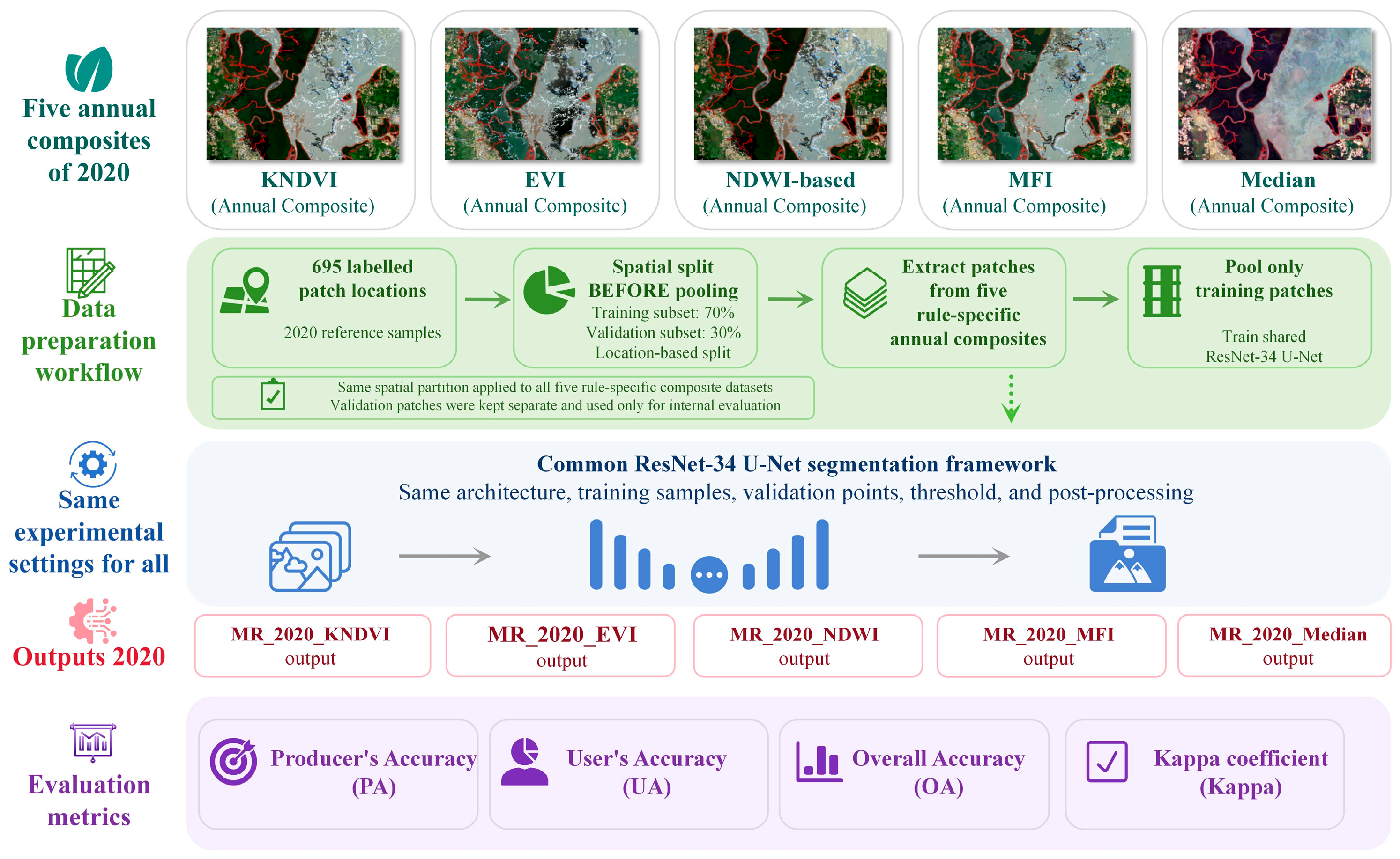
For model development, the same 695 labelled patch locations were sampled from each of the five rule-specific 2020 annual composites, including MAX-KNDVI, MAX-EVI, the NDWI-based composite, MAX-MFI, and Median composites. Each input patch contained 12 Sentinel-2 spectral bands and had a size of 128 × 128 pixels. The corresponding binary labels represented mangrove and non-mangrove classes. Before generating the pooled training dataset, the 695 labelled spatial locations were first divided into training (70%) and internal validation (30%) subsets. This spatial partition was then consistently applied to all five rule-specific composite datasets, ensuring that the same geographic locations were assigned to the same subset across different compositing strategies. The training patches from the five composites were pooled to train a single shared ResNet-34 U-Net model, thereby avoiding additional variability from independently trained rule-specific models. After training, the model weights were fixed and applied separately to each composite, so the comparison reflects relative performance under a common model rather than rule-specific model optimization.

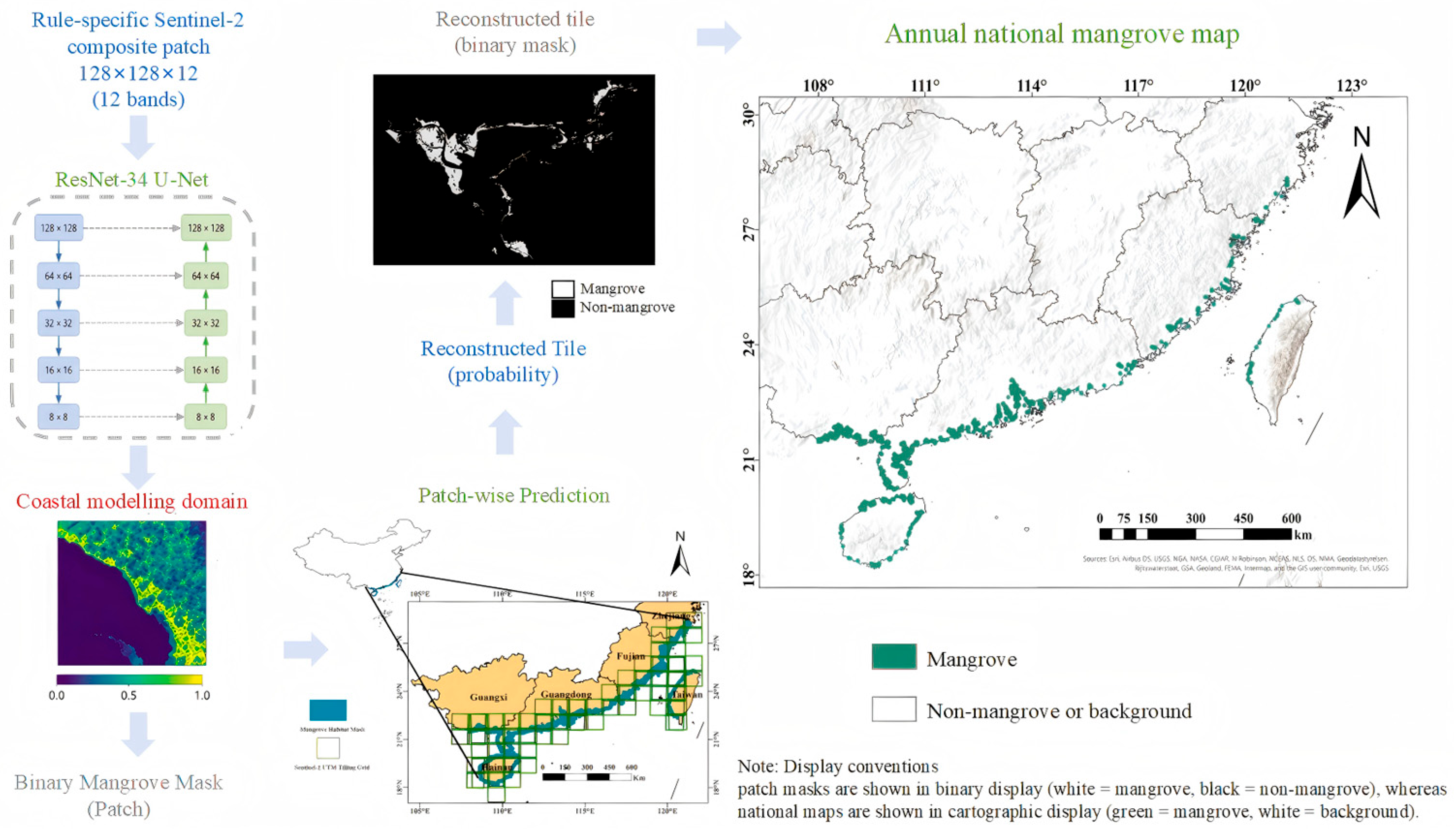
The segmentation model followed a ResNet-34 U-Net architecture. ResNet-34 was used as the encoder to extract hierarchical spectral-spatial features, and the U-Net decoder restored spatial detail for pixel-level prediction [32,33]. All input bands were normalized using statistics calculated from the training data. During prediction, patch-level probability maps were merged to reconstruct tile-level mangrove maps.

The MR_DLM_2020 model was implemented using the PyTorch 2.13.0 deep learning framework and trained on a workstation equipped with an Intel i9-13900HX CPU and an NVIDIA GeForce RTX 4060 Laptop GPU with 8 GB of VRAM. The model was optimized using the Adam optimizer for 1000 epochs [34]. To reduce overfitting and alleviate class imbalance between mangrove and non-mangrove pixels, Mixup augmentation and weighted cross-entropy loss were applied during training [35]. Mixup generated augmented training samples by linearly combining two image patches and their labels, whereas weighted cross-entropy reduced the dominance of the non-mangrove background class during optimization.

The core formulation for this approach is provided in Equations (1)–(4).

$$\tilde{x}=\lambda x_i+(1-\lambda )x_j$$

(1)

$$\tilde{y}=\lambda y_i+(1-\lambda )y_j$$

(2)

$$\lambda \sim \mathrm{B}\mathrm{e}\mathrm{t}\mathrm{a}(\alpha ,\alpha )$$

(3)

where $x_i$, $y_i$ and $x_j$, $y_j$ represent two randomly selected input samples and their corresponding labels, respectively. The mixed sample is $\tilde{x}$, and the corresponding label is $\tilde{y}$. where $\lambda$ is sampled from a Beta distribution, $\lambda \sim \mathrm{B}\mathrm{e}\mathrm{t}\mathrm{a}(\alpha ,\alpha )$, and $\alpha$ is the shape parameter.

$$L=-{\displaystyle \frac{1}{N}}{\displaystyle \sum _{i=1}^N}{\displaystyle \sum _{c=1}^C}{w}_c{y}_{ic}\log \left(p_{ic}\right)$$

(4)

where $L$ is the total weighted Cross-Entropy loss, which is the average of the weighted Cross-Entropy loss over all pixels. $N$ represents the total number of samples, i.e., the total number of pixels in the image. $i$ represents the index of a pixel, $i=1,2,\dots ,N$, $C$ represents the number of classes in the image classification task. $w_c$ denotes the weight of class $c$, which is primarily used to address the class imbalance problem and is calculated based on the pixel frequency of each class. $y_{ic}$ represents the true label indicating $i$ whether the pixel belongs to class $c$, it is 1 if the pixel belongs to class $c$, otherwise it is 0. $p_{ic}$ denotes the output probability that pixel $i$ belong to $c$.

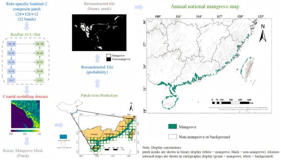
After training, the same MR_DLM_2020 model was applied separately to each rule-specific 2020 annual composite, generating MR_2020_KNDVI, MR_2020_EVI, MR_2020_NDWI, MR_2020_MFI, and MR_2020_Median outputs for controlled comparison (Figure 4). The final layer produced mangrove probability maps. A fixed probability threshold of 0.5 was applied to all rule-specific outputs and all annual maps. Although rule-specific thresholds might improve the accuracy of individual composites, a common threshold was used to maintain a controlled comparison across compositing rules and years and to avoid introducing rule-specific threshold optimization as an additional variable. Thus, the comparison reflects the relative performance of different composites under the same decision threshold in place of their maximum performance after separate threshold optimization (Figure 5).

2.4. Independent Validation, Temporal Mapping, and Exploratory Association Analysis

Internal validation was conducted using the validation subset reserved during model training. Precision, recall, $F_1$-score, and intersection over union (IoU) were calculated at the pixel level to evaluate segmentation performance. Precision measured the reliability of predicted mangrove pixels, recall measured the completeness of detected reference mangrove pixels, $F_1$ score balanced precision and recall, and IoU measured the spatial overlap between predicted and reference mangrove pixels. These metrics were used to assess the behaviour of the shared segmentation model during model development.

Where $\mathrm{T}\mathrm{P}$, $\mathrm{F}\mathrm{P}$, $\mathrm{F}\mathrm{N}$, and TN denote true positives, false positives, false negatives, and true negatives, respectively.

$$\mathrm{P}\mathrm{r}\mathrm{e}\mathrm{c}\mathrm{i}\mathrm{s}\mathrm{i}\mathrm{o}\mathrm{n}={\displaystyle \frac{\mathrm{T}\mathrm{P}}{\mathrm{T}\mathrm{P}+\mathrm{F}\mathrm{P}}}$$

(5)

$$\mathrm{R}\mathrm{e}\mathrm{c}\mathrm{a}\mathrm{l}\mathrm{l}={\displaystyle \frac{\mathrm{T}\mathrm{P}}{\mathrm{T}\mathrm{P}+\mathrm{F}\mathrm{N}}}$$

(6)

$$F_1={\displaystyle \frac{2\mathrm{P}\mathrm{r}\mathrm{e}\mathrm{c}\mathrm{i}\mathrm{s}\mathrm{i}\mathrm{o}\mathrm{n}\mathrm{R}\mathrm{e}\mathrm{c}\mathrm{a}\mathrm{l}\mathrm{l}}{\mathrm{P}\mathrm{r}\mathrm{e}\mathrm{c}\mathrm{i}\mathrm{s}\mathrm{i}\mathrm{o}\mathrm{n}+\mathrm{R}\mathrm{e}\mathrm{c}\mathrm{a}\mathrm{l}\mathrm{l}}}$$

(7)

$$\mathrm{I}\mathrm{o}\mathrm{U}={\displaystyle \frac{\mathrm{T}\mathrm{P}}{\mathrm{T}\mathrm{P}+\mathrm{F}\mathrm{P}+\mathrm{F}\mathrm{N}}}$$

(8)

External validation samples were obtained from the remaining 29 survey regions that were not used for model training. Reference points were selected and interpreted using field-survey information, handheld GPS records, and high-resolution Google Earth imagery. A survey-region-based spatially independent validation design was adopted, resulting in 10,354 reference points, including 5208 mangrove and 5146 non-mangrove points. The separation between the training and validation survey regions was used to reduce the risk of inflated accuracy caused by spatially proximate samples. The same set of validation points was used to evaluate all five rule-specific outputs and the three existing mangrove products. Confusion matrices were generated for each output, and producer accuracy (PA), user accuracy (UA), overall accuracy (OA), and the Kappa coefficient were calculated. The confusion matrix used for external validation is shown in

Table 2. Confusion matrix used for external validation.

Confusion Matrix	Reference
	Mangrove	Non-Mangrove	Total
Mangrove	a ($\mathrm{T}\mathrm{P}$)	b ($\mathrm{F}\mathrm{P}$)	a + b
Non-mangrove	c ($\mathrm{F}\mathrm{N}$)	d (TN)	c + d
Total	a + c	b + d	$\mathrm{N}$

Note: TP, FP, FN, and TN denote true positives, false positives, false negatives, and true negatives for the mangrove class, respectively.

.

For the mangrove class, $PA$ and $UA$ were calculated as:

$$\mathrm{P}{\mathrm{A}}_{\mathrm{m}\mathrm{a}\mathrm{n}\mathrm{g}\mathrm{r}\mathrm{o}\mathrm{v}\mathrm{e}}={\displaystyle \frac{a}{a+c}}$$

(9)

$$\mathrm{U}{\mathrm{A}}_{\mathrm{m}\mathrm{a}\mathrm{n}\mathrm{g}\mathrm{r}\mathrm{o}\mathrm{v}\mathrm{e}}={\displaystyle \frac{a}{a+b}}$$

(10)

For the non-mangrove class, $\mathrm{P}\mathrm{A}$ and $\mathrm{U}\mathrm{A}$ were calculated as:

$$\mathrm{P}{\mathrm{A}}_{\mathrm{n}\mathrm{o}\mathrm{n}-\mathrm{m}\mathrm{a}\mathrm{n}\mathrm{g}\mathrm{r}\mathrm{o}\mathrm{v}\mathrm{e}}={\displaystyle \frac{d}{b+d}}$$

(11)

$$\mathrm{U}{\mathrm{A}}_{\mathrm{n}\mathrm{o}\mathrm{n}-\mathrm{m}\mathrm{a}\mathrm{n}\mathrm{g}\mathrm{r}\mathrm{o}\mathrm{v}\mathrm{e}}={\displaystyle \frac{d}{c+d}}$$

(12)

$OA$ was calculated as:

$$\mathrm{O}\mathrm{A}={\displaystyle \frac{a+d}{N}}$$

(13)

The expected agreement was calculated as:

$$P_e={\displaystyle \frac{(a+b)(a+c)+(c+d)(b+d)}{N^2}}$$

(14)

The Kappa coefficient was calculated as:

$$\kappa ={\displaystyle \frac{OA-P_e}{1-P_e}}$$

(15)

The best-performing compositing rule was selected for annual mangrove mapping from 2019 to 2023. Because Google Earth imagery may not correspond exactly to the target classification year, UAV orthophotos were used as supplementary validation for selected mangrove patches detected by the model but absent from existing products. UAV surveys were conducted using a DJI Mavic 3 Pro between July and October 2023, and the orthophotos were compared with the 2023 model output to assess the delineation of selected small mangrove patches.

Annual mangrove maps were converted to polygons for area and patch-size analysis. The spatial data were stored in WGS-84 for display, whereas area statistics were calculated within the corresponding UTM zones to reduce area distortion. Contiguous mangrove patches were grouped into six size classes: 0–5, 5–50, 50–100, 100–200, 200–300, and >300 ha. These statistics were used to describe changes in mapped area and patch-size distribution, but they were not interpreted as a complete fragmentation assessment.

Finally, exploratory correlation analysis was conducted to examine broad linear associations between mapped mangrove area and selected climatic and anthropogenic variables. Annual total precipitation, annual mean land surface temperature, annual maximum land surface temperature, annual minimum land surface temperature, cropland area, and built-up area were aggregated to 10 km grid cells together with mapped mangrove area. Pearson correlation coefficients were calculated between mapped mangrove area and each selected variable:

$$r_{X,Y}={\displaystyle \frac{\mathrm{c}\mathrm{o}\mathrm{v}(X,Y)}{{\sigma }_X{\sigma }_Y}}$$

(16)

where $\mathrm{c}\mathrm{o}\mathrm{v}\left(X,Y\right)$ is the covariance between variables $X$ and $Y$, ${\sigma }_X$ and ${\sigma }_Y$ are their standard deviations. These correlations were interpreted as exploratory linear associations as opposed to evidence of causal drivers. Nonlinear effects, interaction effects, and spatially explicit driver attribution were not considered in this analysis.

3. Results

3.1. Visual Differences Among Annual Compositing Rules

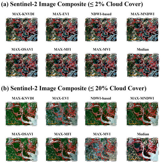
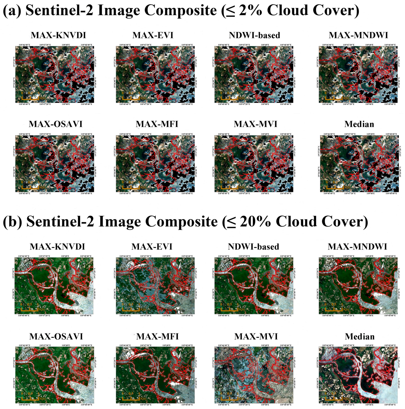
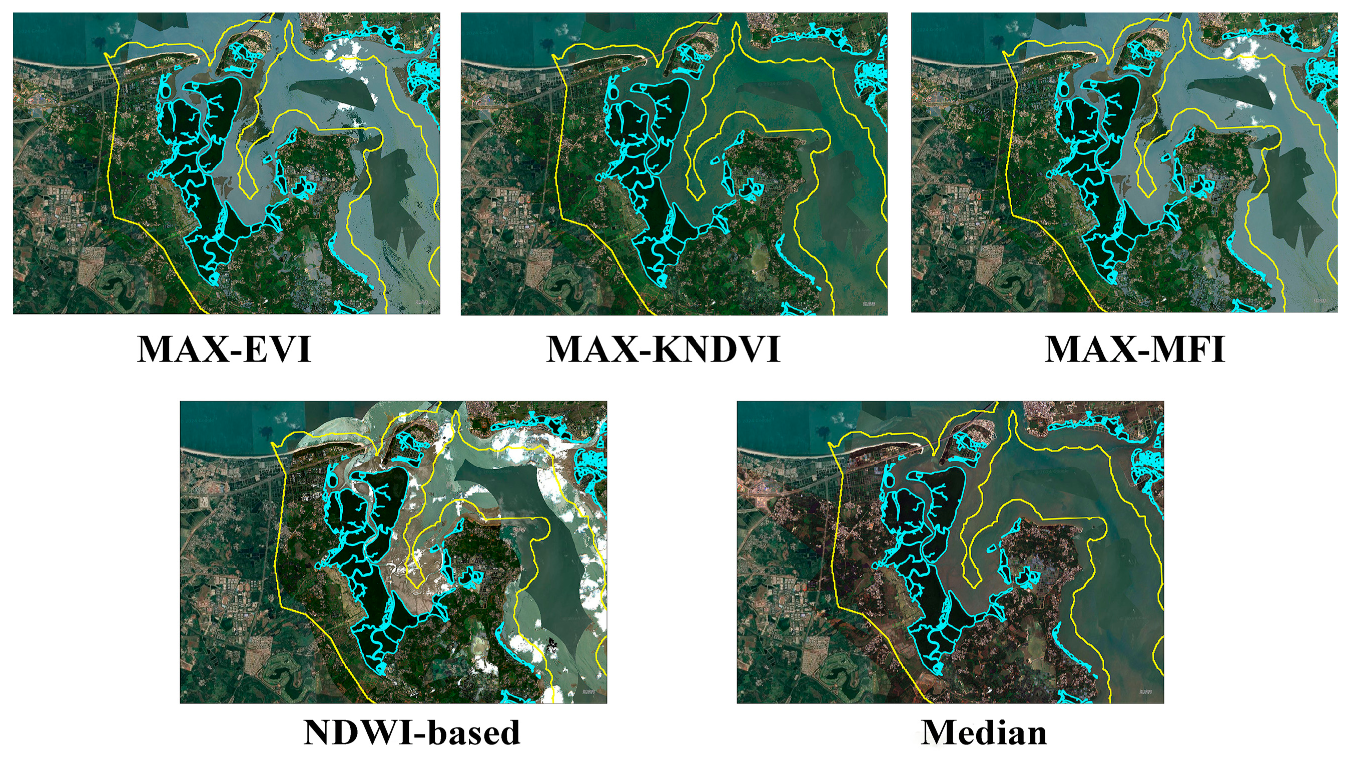
The five Sentinel-2 annual compositing rules produced distinct visual representations of coastal mangrove environments (Figure 6 and Figure 7). In Qinglan Harbour, residual cloud, haze, and water-background effects affected maximum-quality-band composites differently across cloud-cover levels. MAX-KNDVI and MAX-EVI emphasized vegetation greenness and canopy condition, the NDWI-based composite enhanced water-background and inundation signals, and MAX-MFI highlighted red-edge and intertidal mangrove-related responses.

In Dongzhai Harbour, the Median composite showed fewer visible cloud and haze artefacts than most maximum-quality-band composites and produced more spatially continuous coastal boundaries. Some water-mixing and residual atmospheric effects remained in the MAX-EVI, MAX-MFI, and NDWI-based composites. These visual comparisons indicate that all five compositing rules generated usable annual inputs for mangrove segmentation, but their sensitivity to clouds, tidal conditions, and water-background effects differed. Overall, the Median composite provided a more temporally stable representation of the coastal surface, whereas maximum-quality-band composites tended to preserve rule-specific spectral extremes.

3.2. Internal Validation of the Shared Segmentation Model

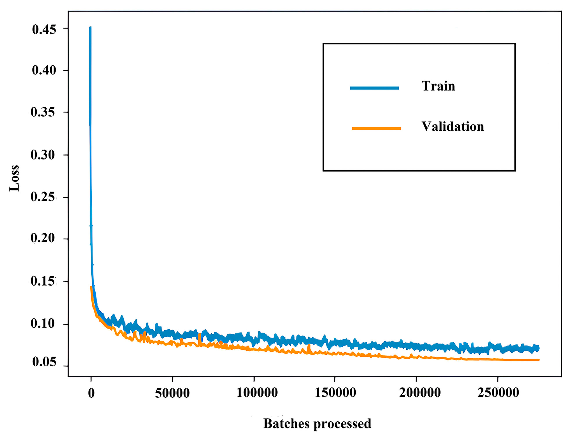
MR_DLM_2020 was implemented in PyTorch and trained using pooled rule-specific patches on a workstation equipped with an Intel i9-13900HX CPU and an NVIDIA GeForce RTX 4060 Laptop GPU. The training loss decreased rapidly during the early stage and became relatively stable after approximately 100,000 iterations (Figure 8). Training was completed after 1000 epochs, and the final shared model weights were used for rule-specific prediction and annual mapping.

The internal validation results are shown in

Table 3. Internal validation results of MR_DLM_2020.

	Mangrove	Non-Mangrove
Precision	0.92	0.98
Recall	0.89	0.99
F1-score	0.91	0.99
IoU	0.83	--

. For mangrove pixels, precision, recall, F1-score, and IoU were 0.92, 0.89, 0.91, and 0.83, respectively. For non-mangrove pixels, the corresponding precision, recall, and F1-score were 0.98, 0.99, and 0.99. These results indicate that the shared segmentation model achieved high internal validation accuracy. The lower recall than precision for mangroves suggests that some mangrove pixels were missed in the validation patches, especially near fragmented boundaries and mixed coastal pixels.

3.3. External Validation and Comparison with Existing Mangrove Products

External validation was conducted using 10,354 spatially independent reference points from 29 coastal regions not used for model training. These points included 5208 mangrove and 5146 non-mangrove samples. The five rule-specific outputs and the three existing mangrove products were evaluated using the same validation samples. All confusion matrices and associated accuracy metrics were calculated using these samples rather than taken directly from the original publications of the existing mangrove products.

The external validation results are summarized in

Table 4. Confusion matrix counts used for external validation.

Dataset/Output	TP	FP	FN	TN	N
HGMF_2020	4425	627	783	4519	10,354
GMW v3.0_2020	3141	614	2067	4532	10,354
LREIS_v2_2020	3971	409	1237	4737	10,354
MR_2020_KNDVI	3580	196	1628	4950	10,354
MR_2020_MFI	3295	156	1913	4990	10,354
MR_2020_EVI	3302	166	1906	4980	10,354
MR_2020_NDWI	3515	195	1693	4951	10,354
MR_2020_Median	4433	254	775	4892	10,354

and

Table 5. External validation accuracy of rule-specific outputs and existing mangrove products.

Dataset/Output	Mangrove PA (%)	Mangrove UA (%)	Non-Mangrove PA (%)	Non-Mangrove UA (%)	OA (%)	Kappa
HGMF_2020	85.0	87.6	87.8	85.2	86.4	0.728
GMW v3.0_2020	60.3	83.6	88.1	68.7	74.1	0.483
LREIS_v2_2020	76.2	90.7	92.1	79.3	84.1	0.682
MR_2020_KNDVI	68.7	94.8	96.2	75.3	82.4	0.648
MR_2020_MFI	63.3	95.5	97.0	72.3	80.0	0.601
MR_2020_EVI	63.4	95.2	96.8	72.3	80.0	0.601
MR_2020_NDWI	67.5	94.7	96.2	74.5	81.8	0.636
MR_2020_Median	85.1	94.6	95.1	86.3	90.1	0.801

. Among the five rule-specific outputs, MR_2020_Median achieved the highest overall performance, with an overall accuracy (OA) of 90.1% and a Kappa coefficient of 0.801. Its mangrove producer accuracy (PA) and user accuracy (UA) were 85.1% and 94.6%, respectively. The three existing mangrove products showed lower or more uneven agreement with the independent validation samples.

The maximum-quality-band outputs generally showed high UA but relatively low PA for the mangrove class. This pattern indicates that pixels classified as mangroves by these outputs were usually reliable, but many reference mangrove samples were omitted. In contrast, MR_2020_Median provided a more balanced result by improving mangrove PA while maintaining high UA, suggesting that the Median composite better preserved stable mangrove signals across heterogeneous coastal settings.

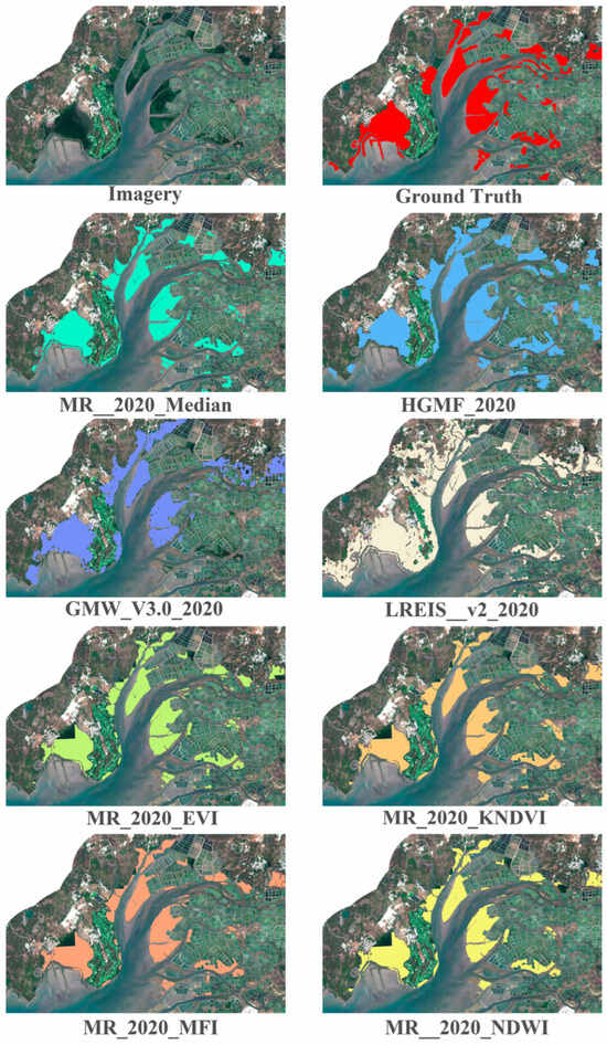
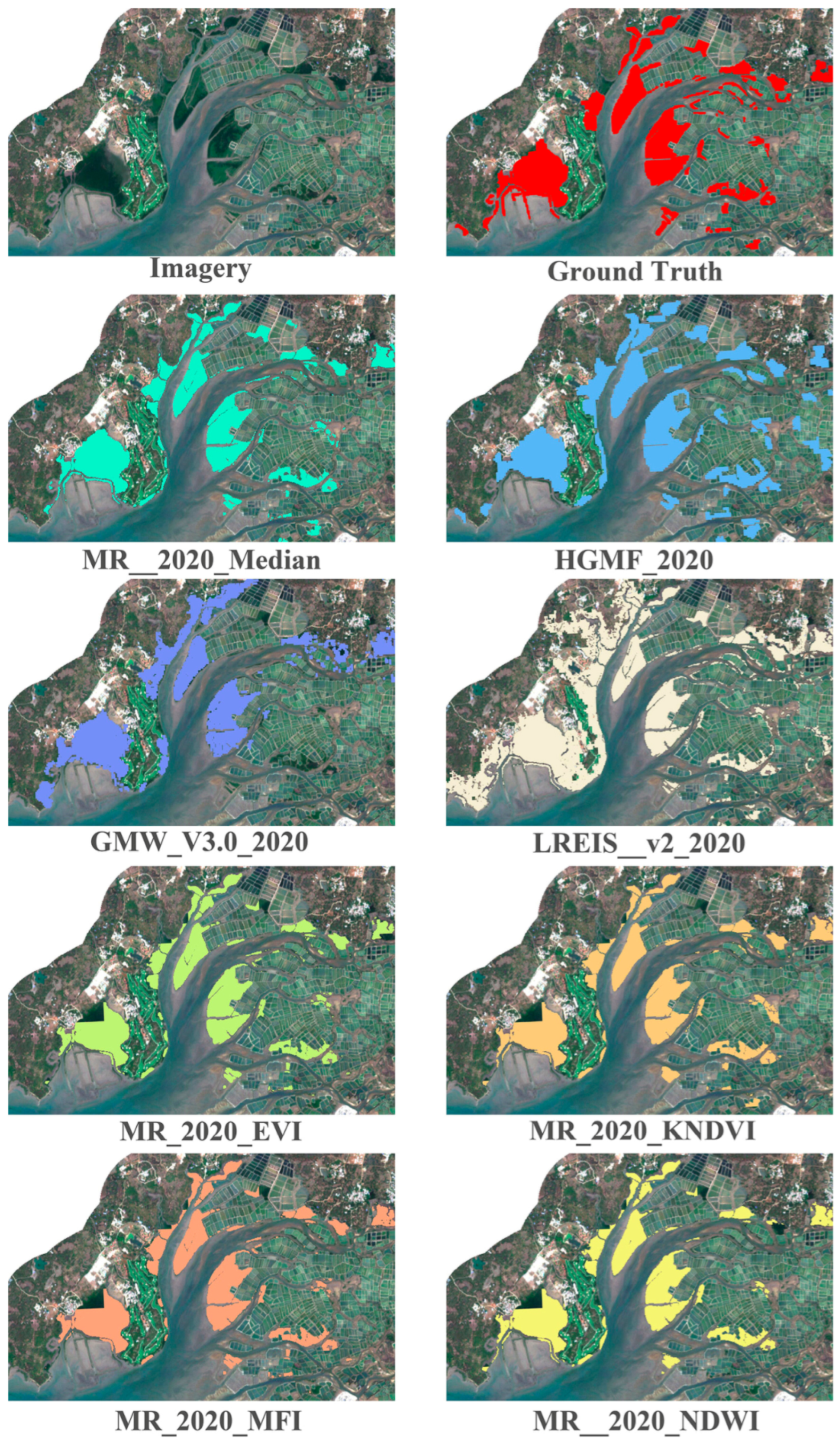
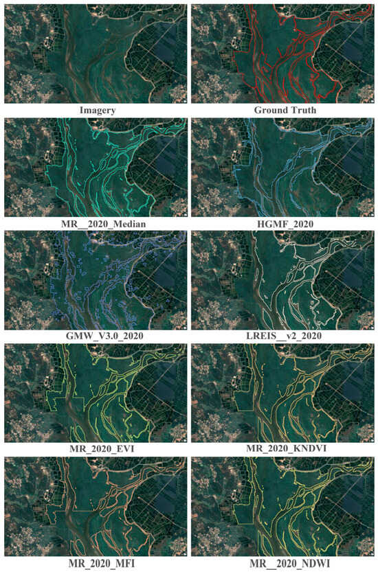
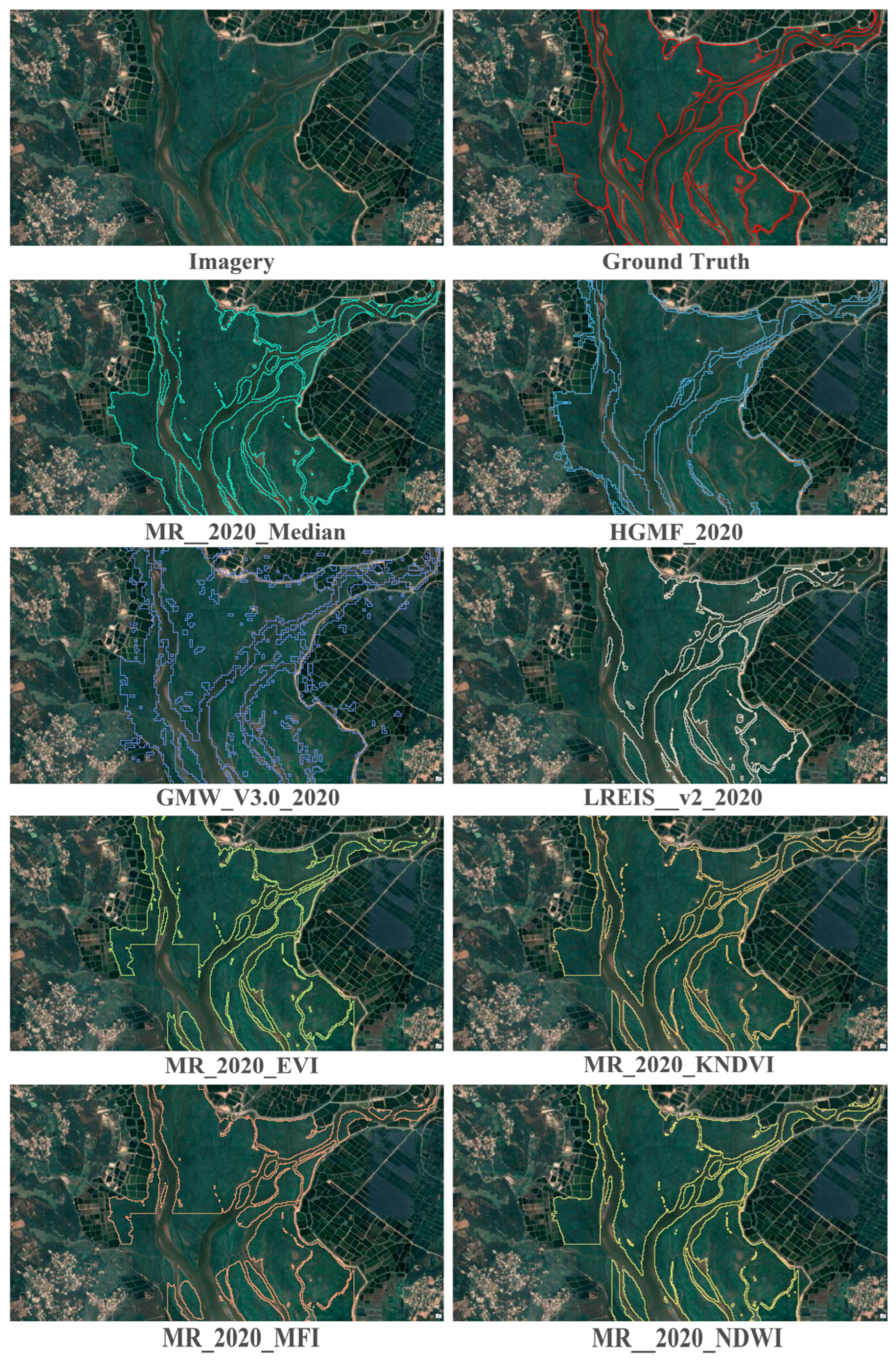
Compared with existing products, MR_2020_Median improved OA by 3.7 percentage points relative to HGMF_2020, 6.0 percentage points relative to LREIS_v2_2020, and 16.0 percentage points relative to GMW v3.0_2020. The improvement was most evident in selected fragmented coastal zones, where MR_2020_Median showed fewer visible omissions and more coherent boundaries (Figure 9 and Figure 10). These results support the selection of MR_2020_Median as the representative configuration for annual mapping and subsequent analyses.

3.4. Temporal Mapping and UAV Verification

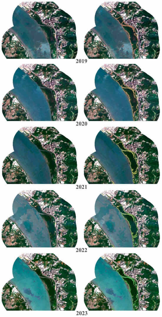
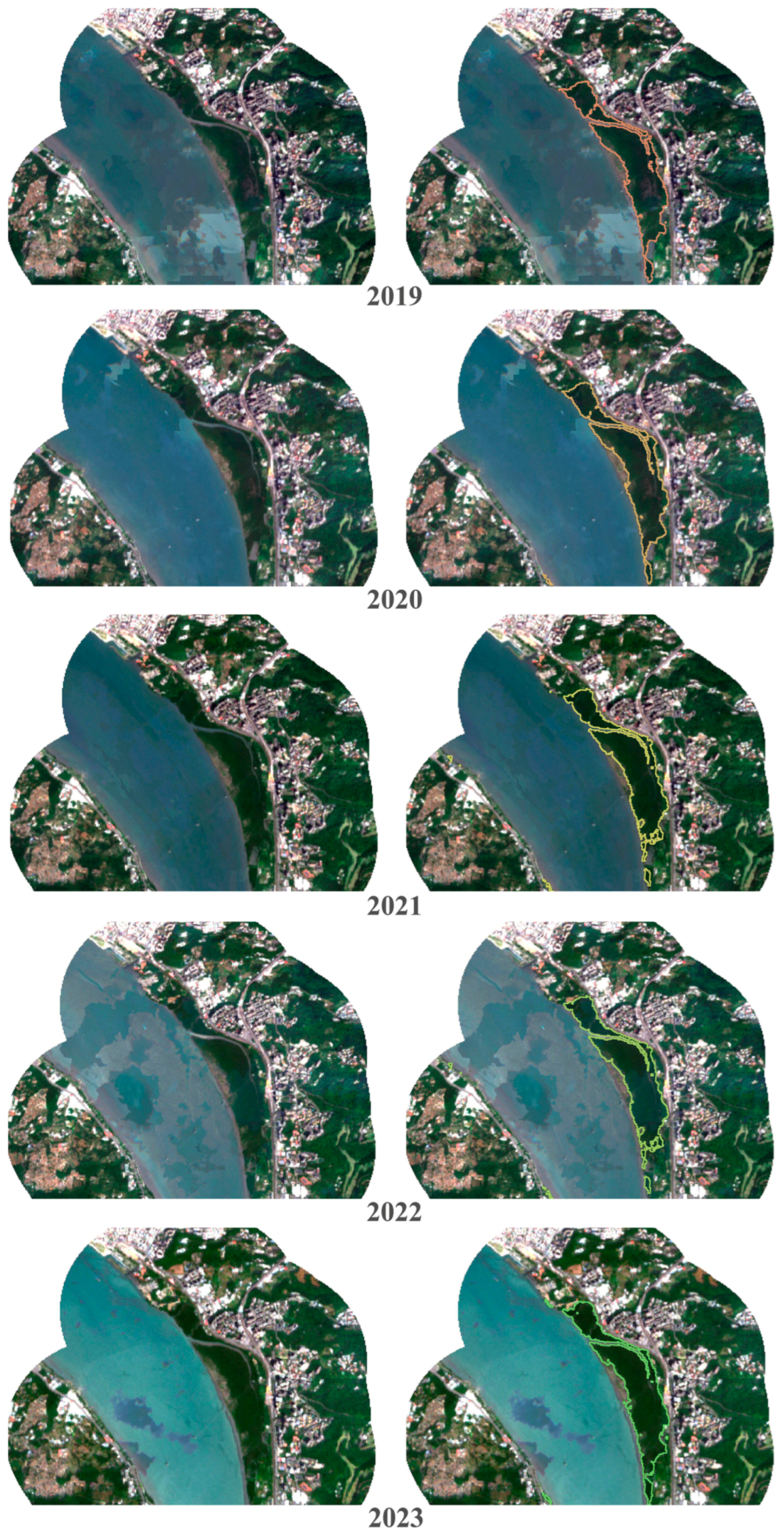
Based on the external validation and visual comparison results, MR_2020_Median was selected as the representative configuration for annual mangrove mapping. The trained MR_DLM_2020 model was applied to Sentinel-2 annual Median composites from 2019 to 2023 to generate national-scale mangrove maps of China. Visual inspection showed that the mapped mangrove boundaries were generally stable across the examined years and coastal regions, although local uncertainty remained in narrow belts, mixed pixels, and tidally variable shorelines.

Taiwan was used as an additional qualitative test area because it was not included in field-sample collection or model training and contains estuarine and urban coastal settings that differ from the main training regions (Figure 11). The model produced visually coherent mangrove boundaries in the Tamsui River Mangrove Nature Reserve, suggesting preliminary spatial transferability under the selected Median compositing configuration. However, this qualitative test should be interpreted cautiously because local turbidity, tidal stage, evergreen vegetation background, and image conditions may still influence classification performance.

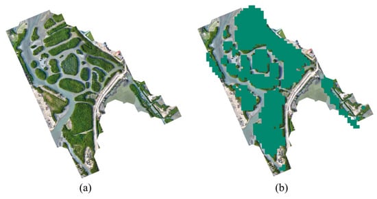
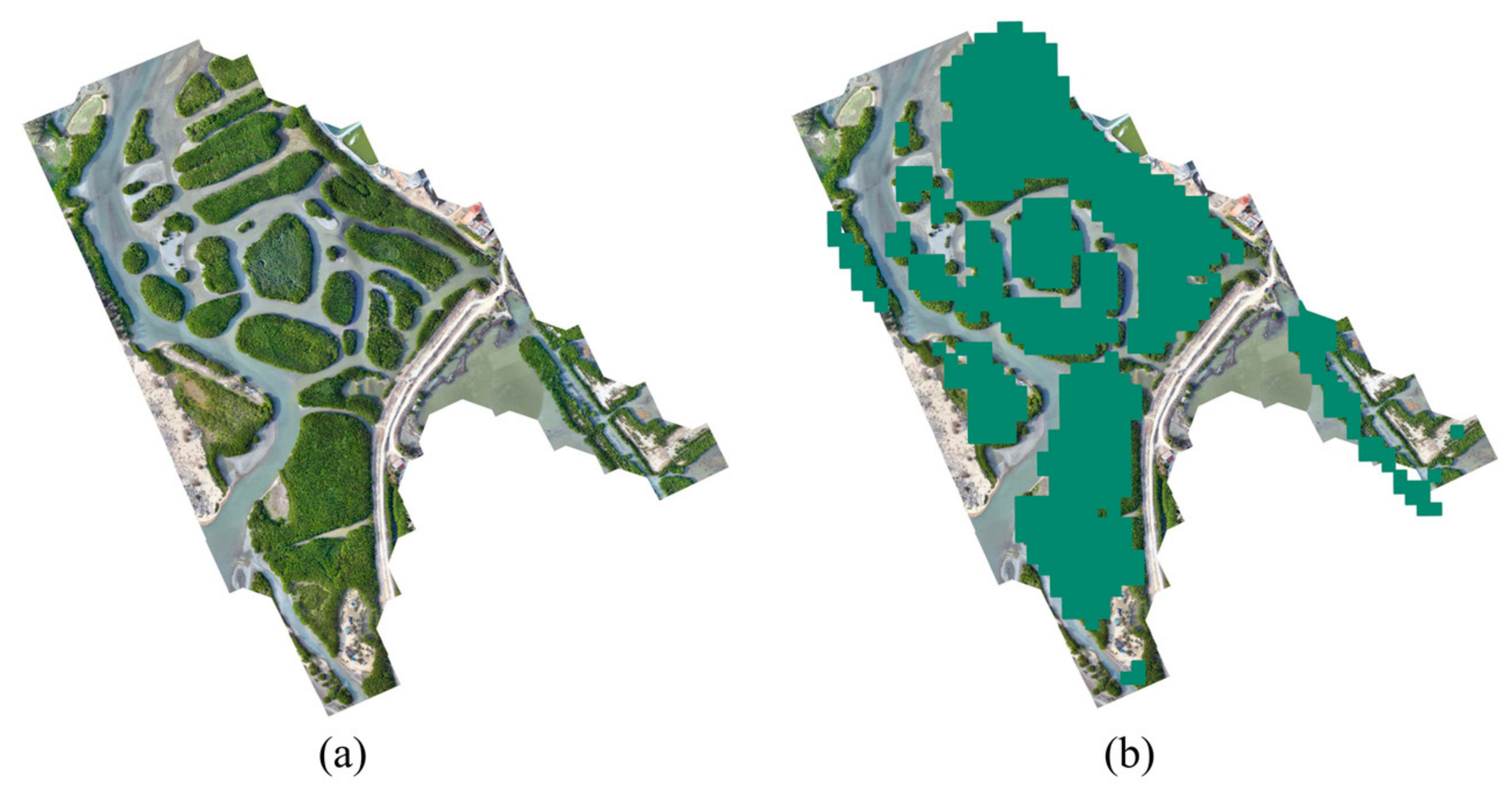
UAV orthophotos were used as supplementary evidence for selected mangrove patches on Hainan Island that were detected by MR_2020_Median but absent from existing mangrove products. The 2023 classification result was generally consistent with the UAV orthophotos in the selected verification sites (Figure 12). For example, newly mapped patches at Liaozi Slope, Ledong County, were clearly visible in the UAV images. These comparisons provide additional evidence that the selected configuration can identify small and fragmented mangrove patches omitted by existing products, although the UAV comparison was site-specific, falling short of a complete national validation.

3.5. Mangrove Area, Patch-Size Distribution, and Exploratory Associations

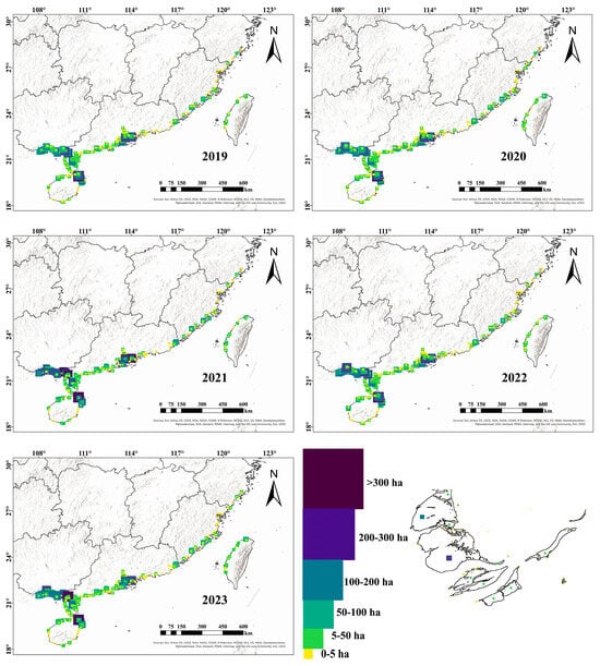
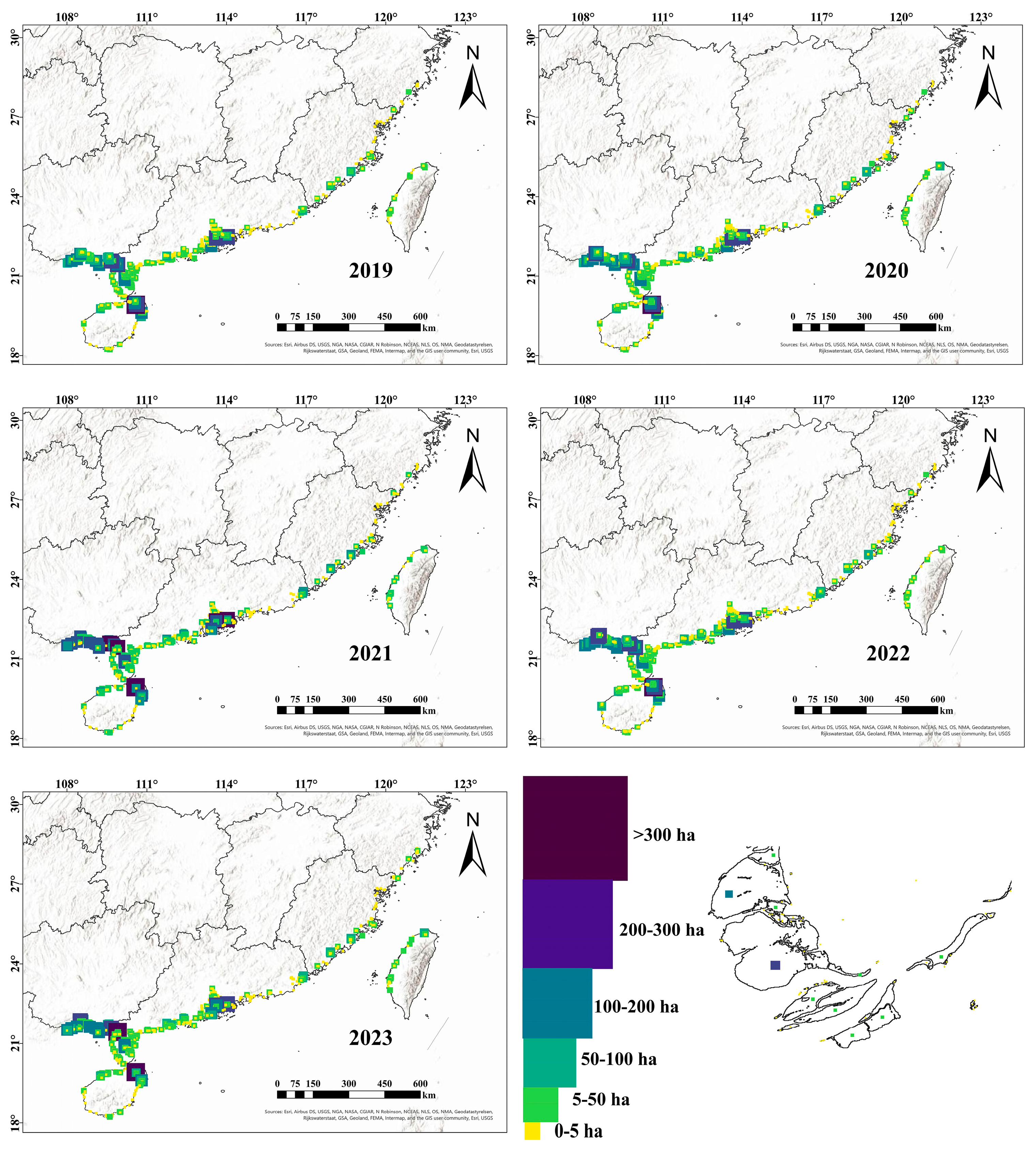
Using the selected Median compositing configuration, annual mangrove maps of China were generated from 2019 to 2023 (Figure 13). The mapped mangrove polygons were stored in WGS-84 for spatial display, and area statistics were calculated within the corresponding UTM zones to reduce area distortion. The mapped mangrove forest area in China increased from 22,731.76 ha in 2019 to 24,631.62 ha in 2023, representing a net increase of 1899.86 ha (

Table 6. Mapped mangrove forest area in China from 2019 to 2023.

Provinces/Country	Area (ha)
	2019	2020	2021	2022	2023
Hainan	3953.08	4052.33	4121.66	4237.99	4311.33
Guangxi	8044.75	8176.43	8471.49	9062.57	9170.75
Guangdong	9538.59	9580.78	9898.35	10,632.53	9606.83
Fujian	758.58	824.29	770.95	895.23	978.02
Zhejiang	83.18	58.17	78.09	87.02	107.31
Taiwan	353.58	379.46	477.37	477.44	457.79
China	22,731.76	23,071.46	23,818.08	25,392.78	24,631.62

). Guangxi showed the largest increase, from 8044.75 ha to 9170.75 ha. Hainan, Fujian, Zhejiang, and Taiwan also showed net increasing trends. Guangdong changed only slightly over the full study period, although a marked decrease occurred between 2022 and 2023, which may reflect local coastal change, image conditions, or boundary uncertainty.

Contiguous mangrove patches were grouped into six size classes: 0–5, 5–50, 50–100, 100–200, 200–300, and >300 ha. At the national scale, the number of contiguous patches increased from 16,198 in 2019 to 16,586 in 2023 (

Table 7. Number of contiguous mangrove patches.

Provinces/ Country	Uninterrupted Mangrove Area Count
	Area Size (ha)	2019	2020	2021	2022	2023
Hainan	0–5	1834	1832	1933	2095	2759
	5–50	97	105	101	106	106
	50–100	6	5	9	8	6
	100–200	4	5	4	4	4
	200–300	1	1	1	1	2
	>300	1	1	1	1	1
	Total	1943	1949	2049	2215	2878
Guangxi	0–5	4262	3993	3790	3987	3712
	5–50	271	250	281	290	282
	50–100	24	20	21	20	24
	100–200	10	14	14	14	17
	200–300	1	2	2	3	2
	>300	0	0	0	0	0
	Total	4568	4279	4108	4314	4037
Guangdong	0–5	8356	8113	7682	9692	8130
	5–50	284	298	306	320	298
	50–100	6	9	10	13	9
	100–200	5	6	5	4	4
	200–300	3	6	3	4	2
	>300	0	0	0	0	1
	Total	8654	8428	8006	10,033	8444
Fujian	0–5	685	557	548	719	780
	5–50	27	29	20	22	24
	50–100	2	3	3	4	5
	100–200	0	0	0	0	0
	200–300	0	0	0	0	0
	>300	0	0	0	0	0
	Total	714	589	571	745	809
Zhejiang	0–5	28	13	39	53	90
	5–50	1	1	2	2	5
	50–100	0	0	0	0	0
	100–200	0	0	0	0	0
	200–300	0	0	0	0	0
	>300	0	0	0	0	0
	Total	29	13	41	55	95
Taiwan	0–5	276	303	363	362	300
	5–50	14	17	19	19	22
	50–100	0	1	0	0	1
	100–200	0	0	0	0	0
	200–300	0	0	0	0	0
	>300	0	0	0	0	0
	Total	290	321	382	381	323
China	0–5	15,441	14,810	14,355	16,908	15,771
	5–50	694	700	729	759	737
	50–100	38	38	43	45	45
	100–200	19	23	23	22	25
	200–300	5	5	6	8	6
	>300	1	1	1	1	2
	Total	16,198	15,579	15,157	17,743	16,586

). The increases were mainly concentrated in the 0–5 ha and 5–50 ha classes. These results indicate that the total mapped mangrove area increased, while patch-size distributions also changed among provinces. However, patch counts alone are insufficient to infer landscape fragmentation. A formal fragmentation assessment would require additional landscape metrics, such as patch density, mean patch size, edge density, core area, and connectivity.

Exploratory correlation analysis showed weak linear associations between mangrove area and the selected climatic and land-use variables (

Table 8. Pearson correlation coefficients between mapped mangrove area and selected climatic and land-use variables.

Factors	r
Annual max Land Surface Temperature	−0.111
Annual min Land Surface Temperature	−0.020
Annual mean Land Surface Temperature	−0.170
Annual total precipitation	0.132
Cropland area	−0.038
Built-up area	−0.171

). Correlation coefficients ranged from −0.171 to 0.132, indicating consistently weak linear relationships. These results are presented only as exploratory associations and should not be interpreted as evidence of environmental or anthropogenic drivers.

4. Discussion

4.1. Effects of Compositing Rules on Mangrove Mapping

The controlled comparison shows that Sentinel-2 annual compositing-rule selection is an important source of variation in deep learning-based mangrove mapping. Because the model architecture, training samples, validation points, threshold, and post-processing settings were kept consistent, differences among the rule-specific outputs mainly reflect differences in how each annual composite represented the coastal surface. Together, these results support the central premise of the study: image compositing should be treated as an experimental variable, not merely as a neutral preprocessing step. Similar concerns have been raised in studies of maximum-value and median compositing, where the choice of temporal compositing rule can substantially alter the spectral signal passed to classification models [11,12,13].

The superior performance of MR_2020_Median in this study can be explained by the coastal conditions under which mangroves were mapped. Maximum-quality-band composites select observations with extreme quality-band values from the annual image stack. This strategy can enhance vegetation greenness, water-background contrast, or intertidal spectral responses, but it can also retain observations affected by residual cloud, haze, glint, turbidity, or unusual tidal exposure. In fragmented mangrove belts, these short-lived extremes may weaken spectral continuity and increase boundary uncertainty. By contrast, median compositing suppresses transient spectral extremes and provides a more conservative annual representation of the coastal surface. Therefore, the result should not be interpreted as evidence that median compositing is universally optimal; rather, under the national-scale Sentinel-2 setting tested here, it provided the most balanced trade-off between omission and commission errors.

The comparison with GMW v3.0, HGMF_2020, and LREIS_v2_2020 further indicates that compositing design can influence product-level agreement, especially in narrow and fragmented coastal zones. MR_2020_Median showed higher agreement with independent validation samples and reduced omissions in selected examples. The UAV comparison also indicated that several small mangrove patches absent from existing products were detected by the selected configuration. These findings are particularly relevant for China, where mangroves often occur as discontinuous belts, small restored patches, or intertidal stands adjacent to aquaculture ponds, mudflats, and evergreen vegetation. In such settings, improving the stability of annual input composites can be as important as improving the classifier itself.

A common ResNet-34 U-Net was used to isolate compositing-related differences while limiting additional model-related variability, thereby allowing for the evaluation of compositing rules under a unified segmentation framework. This architecture was selected because it provides a stable and computationally practical framework for patch-based semantic segmentation [32,33]. More complex attention-based or Transformer-based models may further improve feature learning, but they would introduce additional model-related variables and require larger training datasets. Likewise, optical-SAR fusion and multi-source feature learning can improve mangrove classification in complex coastal environments [23,24,25], but they also increase preprocessing and computational requirements. The present design therefore emphasizes methodological control: the five outputs were generated by varying the annual composite while keeping the trained model and inference settings fixed.

4.2. Mangrove Changes and Regional Differences from 2019 to 2023

The mapped mangrove forest area in China increased from 2019 to 2023. This pattern is consistent with previous observations that mangrove conservation and restoration have contributed to partial recovery along parts of the Chinese coast [7,8]. However, the mapped increase should be interpreted cautiously. The annual maps quantify changes in mapped forest extent, not necessarily changes in stand quality, species composition, survival rate, or ecological function. Some increases may reflect restoration and planting, whereas others may be influenced by boundary uncertainty, tidal exposure, or improved detection of small patches. For comparison, recent national statistics reported approximately 30,300 ha of mangrove land in China [36], while a previous 10 m national-scale remote-sensing study estimated approximately 21,148–24,801 ha [37]. Our 2023 estimate of 24,631.62 ha is lower than the official statistic but comparable in magnitude to previous high-resolution remote-sensing estimates. Because the geographic and thematic definitions are not fully equivalent, these values should be compared cautiously. Differences among estimates may reflect variations in mangrove definition, mapping resolution, classification thresholds, tidal and mixed-pixel treatment, and minimum mapped patch size.

Patch-size statistics suggest that changes in mangrove spatial pattern were more complex than total area change alone. The number of small patches increased during the study period, especially in the 0–5 ha and 5–50 ha classes. This pattern may indicate newly detected or recently established small stands, but patch counts alone cannot support a formal conclusion about fragmentation. A rigorous fragmentation assessment would require additional landscape metrics, such as patch density, mean patch size, edge density, core area, and connectivity, together with uncertainty estimates for patch boundaries.

The regional differences observed in this study likely reflect the combined influence of restoration effort, local geomorphic conditions, available intertidal space, hydrological connectivity, and coastal land-use pressure. Guangxi contributed the largest mapped area increase, whereas Guangdong showed stronger interannual fluctuation. These differences suggest that national-scale mangrove monitoring should be interpreted together with regional coastal settings and management context. Area expansion is encouraging, but conservation assessment should also consider whether mapped patches are hydrologically connected, structurally mature, and resilient to disturbance.

4.3. Exploratory Associations with Environmental and Anthropogenic Variables

The relationships between mapped mangrove area and selected environmental and land-use variables should be interpreted as exploratory linear associations as opposed to driver attribution. Pearson correlation does not establish causality, and all coefficients in this study were small. The weak negative associations with land surface temperature may reflect temperature stress or regional climatic gradients, whereas the weak positive association with precipitation may indicate generally favourable conditions in humid coastal environments. These weak relationships may also reflect spatial-scale mismatch, aggregation effects, nonlinear responses, and regional heterogeneity that are not captured by simple bivariate correlations.

The weak negative associations with cropland and built-up area may indicate potential pressure from coastal land use, but they do not provide direct evidence of habitat loss. Mangrove dynamics are shaped by interactions among tidal exchange, sediment supply, salinity, geomorphology, protection status, restoration practices, and local disturbance. Therefore, the correlation analysis provides context for interpreting broad spatial patterns but does not replace spatially explicit change analysis or field-based ecological assessment.

Future driver analysis would benefit from longer time series, restoration project records, coastal development data, hydrodynamic variables, and nonlinear modelling approaches. Generalized additive models, tree-based methods, or hierarchical spatial models could be used to examine thresholds, interactions, and regional heterogeneity. Such approaches would be more appropriate for identifying potential drivers than simple bivariate correlations over a short five-year period.

4.4. Limitations and Uncertainties

Several sources of uncertainty remain. First, although the training and validation samples covered multiple coastal regions and environmental settings, some conditions were still underrepresented, including extremely turbid waters, dense evergreen coastal vegetation, unusual phenological patterns, and highly disturbed urban shorelines. The lower performance under spatially independent external validation likely reflects the greater difficulty of transferring the model to geographically distinct coastal regions, while spatial correlation among pixels within the internal validation patches may have contributed to relatively optimistic internal metrics. Direct transfer of the model to other mangrove regions therefore requires further independent validation.

Second, classification uncertainty is concentrated along mangrove boundaries and fragmented belts. At 10 m resolution, mixed pixels are common along mangrove-water and mangrove-upland edges. Tidal stage, water turbidity, salt marshes, aquaculture ponds, and evergreen vegetation can all reduce spectral separability. Although the Median composite improved mapping stability in this study, it may also smooth short-lived seasonal or hydrological signals that are useful in some local settings. Future work should include seasonal composites, uncertainty layers, tide-level information, and higher-resolution validation data to better quantify boundary uncertainty.

Third, this study focused on the controlled comparison of Sentinel-2 annual compositing rules as opposed to feature-level ablation, adaptive rule weighting, or multi-source data fusion. Because the shared model was trained using pooled rule-specific patches, the results evaluate rule-specific annual inputs under a common model, but they do not quantify the independent contribution of each spectral band or index-derived feature. Future work should test adaptive compositing, rule weighting, SAR-optical integration, improved cloud and shadow masking, and broader independent validation to determine whether the framework can be generalized beyond the sampled coastal settings.

5. Conclusions

This study evaluated five Sentinel-2 annual compositing rules for 10 m national-scale mangrove forest mapping in China within a shared ResNet-34 U-Net framework. By keeping the model architecture, training samples, validation points, probability threshold, and post-processing settings consistent, the study isolated compositing rule as the main experimental variable. The controlled comparison showed that annual compositing-rule selection substantially affected deep learning-based mangrove segmentation. Among the tested rule-specific outputs, MR_2020_Median produced the most balanced result, with an overall accuracy of 90.1% and a Kappa coefficient of 0.801.

MR_2020_Median showed higher agreement with spatially independent validation samples than GMW v3.0, HGMF_2020, and LREIS_v2_2020, and reduced omissions in selected fragmented coastal zones. UAV orthophotos further supported the detection of several small mangrove patches absent from existing products. When the selected Median configuration was applied to annual Sentinel-2 composites from 2019 to 2023, the mapped mangrove forest area in China increased from 22,731.76 ha to 24,631.62 ha, with Guangxi contributing the largest increase. Exploratory correlations with climatic and land-use variables were weak and should be interpreted as contextual associations as opposed to causal evidence.

These results show that annual compositing design should be evaluated explicitly in Sentinel-2 deep learning-based mangrove mapping. Median compositing provided a practical and stable input strategy under the specific model, threshold, spatial resolution, and coastal conditions tested in this study; its relative advantage may differ under other experimental settings or geographic regions. Remaining uncertainties are mainly related to mixed pixels, tidal variation, cloud residuals, fragmented boundaries, and underrepresented coastal settings. Future work should incorporate more independent validation data, uncertainty mapping, seasonal or tide-aware composites, and broader tests beyond the sampled coastal regions.

References

- Donato, D.C.; Kauffman, J.B.; Murdiyarso, D.; Kurnianto, S.; Stidham, M.; Kanninen, M. Mangroves among the most carbon-rich forests in the tropics. Nat. Geosci. 2011, 4, 293–297. [Google Scholar] [CrossRef] [Scilit]
- Friess, D.A.; Rogers, K.; Lovelock, C.E.; Krauss, K.W.; Hamilton, S.E.; Lee, S.Y.; Lucas, R.; Primavera, J.; Rajkaran, A.; Shi, S. The state of the world’s mangrove forests: Past, present, and future. Annu. Rev. Environ. Resour. 2019, 44, 89–115. [Google Scholar] [CrossRef] [Scilit]
- Menendez, P.; Losada, I.J.; Beck, M.W.; Torres-Ortega, S.; Espejo, A.; Narayan, S.; Diaz-Simal, P.; Lange, G.M. Valuing the protection services of mangroves at national scale: The Philippines. Ecosyst. Serv. 2018, 34, 24–36. [Google Scholar] [CrossRef] [Scilit]
- Kuenzer, C.; Bluemel, A.; Gebhardt, S.; Quoc, T.V.; Dech, S. Remote sensing of mangrove ecosystems: A review. Remote Sens. 2011, 3, 878–928. [Google Scholar] [CrossRef] [Scilit]
- Tran, T.V.; Reef, R.; Zhu, X. A review of spectral indices for mangrove remote sensing. Remote Sens. 2022, 14, 4868. [Google Scholar] [CrossRef] [Scilit]
- Zhang, X.; Treitz, P.M.; Chen, D.; Quan, C.; Shi, L.; Li, X. Mapping mangrove forests using multi-tidal remotely sensed data and a decision-tree-based procedure. Int. J. Appl. Earth Obs. Geoinf. 2017, 62, 201–214. [Google Scholar] [CrossRef] [Scilit]
- Chen, B.; Xiao, X.; Li, X.; Pan, L.; Doughty, R.; Ma, J.; Dong, J.; Qin, Y.; Zhao, B.; Wu, Z.; et al. A mangrove forest map of China in 2015: Analysis of time series Landsat 7/8 and Sentinel-1A imagery in Google Earth Engine cloud computing platform. ISPRS J. Photogramm. Remote Sens. 2017, 131, 104–120. [Google Scholar] [CrossRef] [Scilit]
- Jia, M.; Wang, Z.; Zhang, Y.; Mao, D.; Wang, C. Monitoring loss and recovery of mangrove forests during 42 years: The achievements of mangrove conservation in China. Int. J. Appl. Earth Obs. Geoinf. 2018, 73, 535–545. [Google Scholar] [CrossRef] [Scilit]
- Hu, L.; Li, W.; Xu, B. Monitoring mangrove forest change in China from 1990 to 2015 using Landsat-derived spectral-temporal variability metrics. Int. J. Appl. Earth Obs. Geoinf. 2018, 73, 88–98. [Google Scholar] [CrossRef] [Scilit]
- Navarro, A.; Young, M.; Macreadie, P.I.; Nicholson, E.; Ierodiaconou, D. Mangrove and saltmarsh distribution mapping and land cover change assessment for south-eastern Australia from 1991 to 2015. Remote Sens. 2021, 13, 1450. [Google Scholar] [CrossRef] [Scilit]
- Holben, B.N. Characteristics of maximum-value composite images from temporal AVHRR data. Int. J. Remote Sens. 1986, 7, 1417–1434. [Google Scholar] [CrossRef] [Scilit]
- Griffiths, P.; Nendel, C.; Hostert, P. Intra-annual reflectance composites from Sentinel-2 and Landsat for national-scale crop and land cover mapping. Remote Sens. Environ. 2019, 220, 135–151. [Google Scholar] [CrossRef] [Scilit]
- Qiu, S.; Zhu, Z.; Olofsson, P.; Woodcock, C.E.; Jin, S. Evaluation of Landsat image compositing algorithms. Remote Sens. Environ. 2023, 285, 113375. [Google Scholar] [CrossRef] [Scilit]
- McFeeters, S.K. The use of the Normalized Difference Water Index (NDWI) in the delineation of open water features. Int. J. Remote Sens. 1996, 17, 1425–1432. [Google Scholar] [CrossRef] [Scilit]
- Jia, M.; Wang, Z.; Wang, C.; Mao, D.; Zhang, Y. A new vegetation index to detect periodically submerged mangrove forest using single-tide Sentinel-2 imagery. Remote Sens. 2019, 11, 2043. [Google Scholar] [CrossRef] [Scilit]
- Camps-Valls, G.; Campos-Taberner, M.; Moreno-Martinez, A.; Walther, S.; Duveiller, G.; Cescatti, A.; Mahecha, M.D.; Munoz-Mari, J.; Garcia-Haro, F.J.; Guanter, L.; et al. A unified vegetation index for quantifying the terrestrial biosphere. Sci. Adv. 2021, 7, eabc7447. [Google Scholar] [CrossRef] [Scilit] [PubMed]
- Huete, A.; Didan, K.; Miura, T.; Rodriguez, E.P.; Gao, X.; Ferreira, L.G. Overview of the radiometric and biophysical performance of the MODIS vegetation indices. Remote Sens. Environ. 2002, 83, 195–213. [Google Scholar] [CrossRef] [Scilit]
- Baloloy, A.B.; Blanco, A.C.; Sta. Ana, R.R.C.; Nadaoka, K. Development and application of a new mangrove vegetation index (MVI) for rapid and accurate mangrove mapping. ISPRS J. Photogramm. Remote Sens. 2020, 166, 95–117. [Google Scholar] [CrossRef] [Scilit]
- Tian, J.; Wang, L.; Diao, C.; Zhang, Y.; Jia, M.; Zhu, L.; Xu, M.; Li, X.; Gong, H. National scale sub-meter mangrove mapping using an augmented border training sample method. ISPRS J. Photogramm. Remote Sens. 2025, 220, 156–171. [Google Scholar] [CrossRef] [Scilit]
- Bunting, P.; Rosenqvist, A.; Hilarides, L.; Lucas, R.M.; Thomas, N.; Tadono, T.; Worthington, T.A.; Spalding, M.; Murray, N.J.; Rebelo, L.-M. Global mangrove extent change 1996–2020: Global Mangrove Watch version 3.0. Remote Sens. 2022, 14, 3657. [Google Scholar] [CrossRef] [Scilit]
- Xiao, H.; Su, F.; Fu, D.; Yu, H.; Ju, C.; Pan, T.; Kang, L. 10-m Global Mangrove Classification Products of 2018–2020 Based on Big Data, version 1; Science Data Bank: Beijing, China, 2021. [Google Scholar] [CrossRef] [Scilit]
- Jia, M.; Wang, Z.; Mao, D.; Ren, C.; Song, K.; Zhao, C.; Wang, C.; Xiao, X.; Wang, Y. Mapping global distribution of mangrove forests at 10-m resolution. Sci. Bull. 2023, 68, 1306–1316. [Google Scholar] [CrossRef] [Scilit] [PubMed]
- Fu, B.; Liang, Y.; Lao, Z.; Sun, X.; Li, S.; He, H.; Sun, W.; Fan, D. Quantifying scattering characteristics of mangrove species from Optuna-based optimal machine learning classification using multi-scale feature selection and SAR image time series. Int. J. Appl. Earth Obs. Geoinf. 2023, 122, 103446. [Google Scholar] [CrossRef] [Scilit]
- Fu, B.; Kuang, H.; Wu, Y.; Deng, T.; Sun, W.; Shen, X.; Gao, E.; He, H.; Jiang, L. Mangrove species classification using novel adaptive ensemble learning with multi-spatial-resolution multispectral and full-polarization SAR images. Int. J. Digit. Earth 2024, 17, 2346277. [Google Scholar] [CrossRef] [Scilit]
- Fu, B.; Zhang, S.; Li, H.; Yao, H.; Sun, W.; Jia, M.; Yang, Y.; He, H.; Li, Y. Exploring the effects of different combination ratios of multi-source remote sensing images on mangrove communities classification. Int. J. Appl. Earth Obs. Geoinf. 2024, 134, 104197. [Google Scholar] [CrossRef] [Scilit]
- Fu, C.; Song, X.; Xie, Y.; Wang, C.; Luo, J.; Fang, Y.; Cao, B.; Qiu, Z. Research on the spatiotemporal evolution of mangrove forests in Hainan Island from 1991 to 2021 based on SVM and Res-UNet algorithms. Remote Sens. 2022, 14, 5554. [Google Scholar] [CrossRef] [Scilit]
- Wan, Z.; Hook, S.; Hulley, G. MODIS/Terra Land Surface Temperature/Emissivity Daily L3 Global 1 km SIN Grid V061; NASA EOSDIS Land Processes DAAC: Sioux Falls, SD, USA, 2021. [CrossRef]
- Funk, C.; Peterson, P.; Landsfeld, M.; Pedreros, D.; Verdin, J.; Shukla, S.; Husak, G.; Rowland, J.; Harrison, L.; Hoell, A.; et al. The Climate Hazards Infrared Precipitation with Stations: A new environmental record for monitoring extremes. Sci. Data 2015, 2, 150066. [Google Scholar] [CrossRef] [Scilit] [PubMed]
- Karra, K.; Kontgis, C.; Statman-Weil, Z.; Mazzariello, J.C.; Mathis, M.; Brumby, S.P. Global land use/land cover with Sentinel-2 and deep learning. In Proceedings of the IEEE International Geoscience and Remote Sensing Symposium (IGARSS), Brussels, Belgium, 11–16 July 2021; pp. 4704–4707. [Google Scholar] [CrossRef] [Scilit]
- Gorelick, N.; Hancher, M.; Dixon, M.; Ilyushchenko, S.; Thau, D.; Moore, R. Google Earth Engine: Planetary-scale geospatial analysis for everyone. Remote Sens. Environ. 2017, 202, 18–27. [Google Scholar] [CrossRef] [Scilit]
- Coluzzi, R.; Imbrenda, V.; Lanfredi, M.; Simoniello, T. A first assessment of the Sentinel-2 Level 1-C cloud mask product to support informed surface analyses. Remote Sens. Environ. 2018, 217, 426–443. [Google Scholar] [CrossRef] [Scilit]
- He, K.; Zhang, X.; Ren, S.; Sun, J. Deep residual learning for image recognition. In Proceedings of the IEEE Conference on Computer Vision and Pattern Recognition (CVPR), Las Vegas, NV, USA, 27–30 June 2016; pp. 770–778. [Google Scholar] [CrossRef] [Scilit]
- Ronneberger, O.; Fischer, P.; Brox, T. U-Net: Convolutional networks for biomedical image segmentation. In Medical Image Computing and Computer-Assisted Intervention—MICCAI 2015; Navab, N., Hornegger, J., Wells, W.M., Frangi, A.F., Eds.; Springer: Cham, Switzerland, 2015; Volume 9351, pp. 234–241. [Google Scholar] [CrossRef] [Scilit]
- Kingma, D.P.; Ba, J. Adam: A method for stochastic optimization. In Proceedings of the International Conference on Learning Representations (ICLR), San Diego, CA, USA, 7–9 May 2015. [Google Scholar]
- Zhang, H.; Cisse, M.; Dauphin, Y.N.; Lopez-Paz, D. Mixup: Beyond empirical risk minimization. In Proceedings of the International Conference on Learning Representations (ICLR), Vancouver, BC, Canada, 30 April–3 May 2018. [Google Scholar]
- Ministry of Natural Resources of the People’s Republic of China. 2024 China Natural Resources Bulletin; Ministry of Natural Resources of the People’s Republic of China: Beijing, China, 2025. Available online: https://www.gov.cn/lianbo/bumen/202503/P020250322461627579892.pdf (accessed on 7 August 2026). (In Chinese)
- Zhao, C.; Qin, C.-Z. 10-m-resolution mangrove maps of China derived from multi-source and multi-temporal satellite observations. ISPRS J. Photogramm. Remote Sens. 2020, 169, 389–405. [Google Scholar] [CrossRef] [Scilit]
Disclaimer/Publisher’s Note: The statements, opinions and data contained in all publications are solely those of the individual author(s) and contributor(s) and not of MDPI and/or the editor(s). MDPI and/or the editor(s) disclaim responsibility for any injury to people or property resulting from any ideas, methods, instructions or products referred to in the content. |
© 2026 by the authors. Licensee MDPI, Basel, Switzerland. This article is an open access article distributed under the terms and conditions of the Creative Commons Attribution (CC BY) license.