Reliability-Aware Dual-Stream Self-Training for Semi-Supervised Semantic Segmentation of High-Resolution Remote Sensing Imagery

Highlights

What are the main findings?

• In high-resolution remote sensing segmentation, conservative pseudo-label filtering improves supervision reliability but may exclude complex scenes, difficult land-cover classes, and small objects, whereas using the complete unlabeled set preserves coverage but introduces unreliable supervision.
• RAPST addresses this conflict through reliable offline supervision, class-adaptive online learning over the complete unlabeled set, and cross-stream feature coordination, achieving the highest mIoU across all eight dataset–annotation settings.

What are the implications of the main findings?

• Semi-supervised remote sensing segmentation does not have to choose between reliable pseudo-labels and broad unlabeled-data coverage.
• Coordinating reliability-oriented and coverage-oriented supervision improves vegetation-class discrimination, structural continuity, and small-object preservation when pixel-level annotations are scarce.

Abstract

Semantic segmentation of high-resolution remote sensing imagery remains constrained by the high cost of pixel-level annotation. Semi-supervised learning can reduce this dependence by exploiting unlabeled images, but improving pseudo-label reliability often comes at the cost of reduced data coverage. Selecting only stable samples can suppress noise but may exclude complex scenes and minority classes, whereas retaining the complete unlabeled set preserves data diversity but introduces less reliable and class-biased supervision. To address this trade-off, we propose RAPST, a reliability-aware dual-stream self-training framework that combines reliable offline supervision with full-data online learning. In the offline stream, the Class-Aware Image Stability Gate (ISG) selects prediction-stable images while preserving class coverage. In the online stream, EMA-Smoothed Class-Adaptive Pseudo-Label Thresholding (CPT) adapts pixel-selection thresholds according to class-wise pseudo-label statistics. Reliability-Aware Prototype-Guided Category Contrast (PCC) further integrates reliable feature–label pairs from both streams to improve feature discrimination. Experiments on the ISPRS Vaihingen, ISPRS Potsdam, and WHDLD datasets under four annotation ratios show that RAPST achieves the best performance in most dataset–annotation settings, with mIoU improvements of 0.33–6.08 percentage points over the supervised-only baseline. Ablation and mechanism analyses further show that prediction stability is associated with pseudo-label quality, CPT increases supervision coverage for difficult classes with limited precision loss, and PCC improves feature-space separability.

1. Introduction

Semantic segmentation of high-resolution remote sensing imagery (HRSI) provides pixel-level land-cover information for urban planning, environmental monitoring, and resource management. Deep segmentation networks, including fully convolutional networks and encoder–decoder architectures, have substantially improved segmentation accuracy through end-to-end feature learning [1,2]. However, their performance depends heavily on large-scale pixel-level annotations. Annotating HRSI is particularly expensive because of the large image size, dense spatial structures, complex boundaries, and diverse land-cover distributions [3]. Semi-supervised semantic segmentation therefore offers a practical solution by exploiting abundant unlabeled images together with limited labeled data.

Existing semi-supervised methods mainly incorporate unlabeled data through consistency regularization and pseudo-label-based self-training. Mean Teacher generates stable supervision using an exponential moving average teacher [4], while ST++ improves self-training by selecting unlabeled samples according to prediction stability [5]. However, reliability-oriented selection may reduce data coverage: stable-sample filtering suppresses pseudo-label noise but can exclude complex scenes, minority classes, and small objects. Conversely, retaining the complete unlabeled set preserves broader scene and class coverage but introduces less reliable and potentially class-biased supervision. This problem is particularly relevant to HRSI, where large class imbalance, small objects, and visually similar land-cover categories make reliable use of unlabeled data difficult.

The challenge is therefore not simply to maximize pseudo-label reliability or unlabeled-data coverage, but to coordinate reliability control at different supervision granularities. Image-level selection determines which samples provide stable offline supervision, whereas pixel-level filtering determines which predictions from the complete unlabeled set remain useful for online learning. Both sources ultimately optimize the same feature representation, where residual pseudo-label noise and class imbalance can further aggravate inter-class confusion. Recent methods have improved adaptive pseudo-labeling and class-aware learning [6,7,8], reliability-based sample selection [9], and prototype-based consistency regularization [10]. Nevertheless, these aspects are generally addressed within a single supervision path or treated separately, leaving the coordinated use of reliable offline supervision, full-data online learning, and feature-level discrimination insufficiently explored.

To address this problem, we propose RAPST, a reliability-aware dual-stream self-training framework that coordinates reliability control across complementary offline and online supervision streams. In the offline stream, the Class-Aware Image Stability Gate (ISG) selects prediction-stable images while preserving class coverage to construct reliable pseudo-labeled supervision. In the online stream, EMA-Smoothed Class-Adaptive Pseudo-Label Thresholding (CPT) operates on the complete unlabeled set and adjusts pixel selection according to class-wise pseudo-label statistics. Reliability-Aware Prototype-Guided Category Contrast (PCC) further integrates reliable feature–label pairs from both streams to improve class discrimination in the shared feature space. Together, these mechanisms coordinate image-level sample reliability, pixel-level online reliability, and feature-level representation learning within a unified framework.

The main contributions of this study are summarized as follows:

(1)

We propose RAPST, a reliability-aware dual-stream self-training framework that coordinates image-level offline reliability, pixel-level online supervision, and cross-stream feature learning under complementary supervision streams.

(2)

Within RAPST, ISG performs class-aware stability-based image selection, CPT provides class-adaptive pixel filtering over the complete unlabeled set, and PCC integrates reliable feature–label pairs from both streams for prototype-guided category contrast. These mechanisms jointly coordinate reliability at the image, pixel, and feature levels.

(3)

Experiments on the ISPRS Vaihingen, ISPRS Potsdam, and WHDLD datasets under four annotation ratios show that RAPST achieves the best performance in most dataset–annotation settings. Ablation and mechanism analyses further evaluate the contributions and intended behaviors of ISG, CPT, and PCC.

2. Related Work

2.1. Semi-Supervised Semantic Segmentation

Semi-supervised semantic segmentation aims to learn pixel-level predictions from a small labeled set and a larger unlabeled set. Compared with image classification, dense prediction is more sensitive to unreliable supervision because pseudo-label errors can accumulate along object boundaries, spatial structures, and feature representations. Existing methods mainly address this problem through consistency regularization and pseudo-label-based self-training. Consistency-based methods enforce prediction agreement under different perturbations or model views, including teacher–student learning, cross pseudo supervision, and weak-to-strong consistency [11,12,13,14,15,16]. Recent variants further extend consistency learning through stronger data perturbations and feature-level regularization [17,18,19].

Pseudo-label-based self-training converts model predictions into additional supervision signals [20,21,22,23]. FixMatch retains high-confidence predictions under a weak-to-strong training paradigm [24], while FlexMatch and CASS further introduce class-adaptive thresholding or sampling to account for differences in learning difficulty [25,26]. Beyond these conventional paradigms, recent studies have also explored diffusion models, state-space architectures such as Mamba, and vision foundation models as stronger generative, representation, or pretrained priors for semi-supervised segmentation [27,28,29,30]. For example, ConformalSAM leverages a pretrained foundation segmentation model to provide supervision for unlabeled images and further calibrates its predictions to reduce unreliable pixel-level supervision [30].

Because pseudo-labels remain imperfect, recent studies have increasingly focused on identifying and reducing unreliable supervision [31,32,33]. GCT detects unreliable regions and combines consistency learning with flaw correction [34], while MKD and DerProp improve supervision reliability through knowledge distillation and feature-guided label propagation, respectively [35,36]. Overall, semi-supervised segmentation has evolved from simply incorporating unlabeled data toward improving how unlabeled supervision is generated, selected, and utilized. Nevertheless, most general methods are developed for natural-image or generic segmentation settings and do not explicitly account for the coupled scale variation, class imbalance, small-object sparsity, and inter-class similarity found in high-resolution remote sensing imagery.

2.2. Semi-Supervised Semantic Segmentation of Remote Sensing Images

Compared with natural images, high-resolution remote sensing images contain denser spatial structures, larger scale variations, and more imbalanced class distributions. Small objects and minority classes are often sparsely represented, while land-cover categories with similar spectral, textural, or spatial characteristics are difficult to distinguish. Accordingly, semi-supervised remote sensing segmentation has gradually shifted from directly transferring general learning frameworks toward methods specifically designed for remote sensing scenarios [37].

Early studies mainly adapted consistency regularization, teacher–student learning, and cross supervision to remote sensing images [38,39]. However, pixel-level consistency alone is insufficient to represent the regional structures and contextual relationships of complex scenes. SegMind introduces masked image modeling into the Mean Teacher framework and combines it with contrastive learning to strengthen regional interaction and feature discrimination [40]. RegionMatch constructs pixel- and region-level consistency constraints to exploit spatial structures within unlabeled images [41]. These studies extend semi-supervised learning beyond isolated pixel predictions by incorporating regional context and representation constraints.

Another line of research addresses pseudo-label noise and class-distribution bias. AdaptMatch improves pseudo-label matching for semi-supervised binary remote sensing segmentation [42], while dynamic multi-scale learning and debiasing frameworks further adapt supervision to class and scale differences [43,44]. DWL reduces the influence of noisy pseudo-labels and long-tailed distributions through decoupled learning and ranked weighting [7]. DAST combines dynamic pseudo-label sampling, distribution matching, and adaptive threshold updating to increase the participation of minority classes [6]. CASSF further integrates hierarchical pseudo-label selection with class contrast to address class imbalance and inter-class confusion in high-resolution remote sensing imagery [8]. These methods demonstrate that reliable pseudo-label learning must account for both prediction confidence and class-dependent learning difficulty.

Recent methods have also focused on uncertain regions, object boundaries, and local structural details. ECAE enhances boundary-sensitive class activation for semi-supervised remote sensing segmentation [45], whereas Semi-BSU combines boundary-aware learning with superpixel refinement [46]. MUCA introduces multi-scale uncertainty consistency and cross-teacher–student attention to improve unlabeled feature learning [47]. CLR-DLR employs contextual label realignment and denoising latent restoration to refine pseudo-labels and boundary predictions [48]. Although these methods improve different aspects of unlabeled-data utilization, offline sample selection, online pixel supervision, and feature representation are generally optimized separately. This separation motivates a coordinated framework that controls reliability across complementary supervision streams while retaining full use of the unlabeled data.

2.3. Reliability-Aware Self-Training and Representation Learning

The effectiveness of self-training depends on whether unreliable predictions can be excluded without discarding valuable supervision. However, pseudo-label reliability varies across images, classes, and spatial regions. Stable images may still contain uncertain boundaries or small objects, while high-confidence predictions may remain incorrect for visually similar classes. Reliable self-training therefore requires more than a single confidence criterion; it must consider how supervision is selected and subsequently used for representation learning.

Image-level methods identify unlabeled samples that are more suitable for self-training. ST++ ranks unlabeled images according to prediction consistency across multiple checkpoints [5], while related approaches progressively introduce stable samples through iterative selection strategies [49]. SISS-Net further divides unlabeled images into reliable and unreliable subsets, using complete pseudo-labels for reliable samples and only high-confidence pixels for unreliable ones [50]. These methods reduce the influence of globally unstable samples. Nevertheless, overall image stability cannot fully characterize class coverage or local pixel reliability, and stability-based selection may favor simple scenes dominated by easily recognized classes.

Pixel-level methods refine pseudo-label supervision through confidence, class statistics, or uncertainty. Confidence-distribution-based selection and uncertainty-weighted learning improve the identification of noisy pseudo-labels beyond fixed global thresholds [51,52]. UCGM combines uncertainty weighting with a cross-image Gaussian mixture model to refine local pseudo-labels [53]. UPC locates uncertain patches and replaces them with reliable labeled regions through uncertainty-aware Patch CutMix [54]. Other studies focus on semantic regions, hard pixels, and internal activation bias to distinguish informative predictions from misleading high-confidence outputs [55,56,57]. Although these methods provide more fine-grained reliability estimation, their selected pixels may still introduce bias when directly used to construct class representations.

Feature-level contrastive and prototype learning further improve intra-class compactness and inter-class separation under limited supervision [58,59,60]. RSProtoSemiSeg represents class distributions using probabilistic prototypes and strengthens pixel–prototype relationships through hybrid contrastive learning for high-spatial-resolution remote sensing images [61]. CPL improves representation consistency through cluster-guided class-aware prototypes [62], while DPC-Net combines global prototype contrast with local prototype consistency [63]. Dual contrastive learning with mutual correction further reduces feature confusion under imperfect supervision [64]. These studies demonstrate the value of prototype-based representation learning, but its effectiveness depends strongly on the reliability of the pixels used to construct prototypes and contrastive anchors.

Taken together, existing studies have improved self-training through stable sample selection, adaptive pixel filtering, uncertainty estimation, and prototype-based representation learning. However, these mechanisms are generally applied within separate supervision paths, leaving the coordination of image-level reliability, pixel-level online supervision, and shared feature learning insufficiently explored. RAPST addresses this gap through complementary offline and online supervision, where ISG controls reliable subset construction, CPT adapts online pixel selection over the complete unlabeled set, and PCC coordinates reliable information from both streams in the shared feature space.

3. Methodology

3.1. Problem Definition

In semi-supervised semantic segmentation of high-resolution remote sensing images, a small labeled dataset and a larger unlabeled dataset are defined as follows:

$$D_l={\left\{\left(x_i^l,y_i^l\right)\right\}}_{i=1}^{N_l},D_u={\left\{x_i^u\right\}}_{i=1}^{N_u},$$

(1)

where $x_i^l$ and $x_i^u$ denote the labeled and unlabeled images, respectively; $y_i^l$ is the pixel-level semantic label corresponding to $x_i^l$; and $N_l$ and $N_u$ denote the numbers of labeled and unlabeled samples, respectively.

The input modality depends on the dataset. For Potsdam and Vaihingen, the input is constructed by stacking infrared–red–green (IRRG) imagery and normalized digital surface model (nDSM) elevation information, whereas WHDLD uses the original three-channel RGB imagery. Accordingly, each input image is represented as follows:

$$x_i^l,x_i^u\in {\mathbb{R}}^{H\times W\times C_{\mathrm{i}\mathrm{n}}},$$

(2)

where $H$ and $W$ denote the spatial height and width of the input image, respectively, and $C_{\mathrm{i}\mathrm{n}}$ denotes the dataset-specific number of input channels. The corresponding pixel-level semantic labels are defined as follows:

$$y_i^l\in {\left\{0,\dots ,C-1\right\}}^{H\times W},$$

(3)

where $C$ denotes the total number of semantic classes.

RAPST uses the unlabeled data through complementary offline and online supervision streams. Let ${\mathcal{I}}_u=\left\{1,\dots ,N_u\right\}$ denote the index set of all unlabeled images. ISG partitions ${\mathcal{I}}_u$ into a reliable subset $S_R$ and a remaining subset $S_U={\mathcal{I}}_u\setminus S_R$, such that $S_R\cap S_U=\mathrm{\varnothing }$ and $S_R\cup S_U={\mathcal{I}}_u$.

Their corresponding offline pseudo-labeled subsets are defined as follows:

$$D_R^u=\left\{\left(x_i^u,{\widehat{y}}_i^R\right)\mid i\in S_R\right\},D_U^u=\left\{\left(x_i^u,{\widehat{y}}_i^U\right)\mid i\in S_U\right\}.$$

(4)

The offline supervision is constructed progressively:

$$D_{\mathrm{o}\mathrm{f}\mathrm{f}\mathrm{l}\mathrm{i}\mathrm{n}\mathrm{e}}^{\left(1\right)}=D_l\cup D_R^u,D_{\mathrm{o}\mathrm{f}\mathrm{f}\mathrm{l}\mathrm{i}\mathrm{n}\mathrm{e}}^{\left(2\right)}=D_l\cup D_R^u\cup D_U^u.$$

(5)

where $D_{\mathrm{o}\mathrm{f}\mathrm{f}\mathrm{l}\mathrm{i}\mathrm{n}\mathrm{e}}^{\left(1\right)}$ is used during reliable-first retraining, whereas $D_{\mathrm{o}\mathrm{f}\mathrm{f}\mathrm{l}\mathrm{i}\mathrm{n}\mathrm{e}}^{\left(2\right)}$ is used as the fixed offline supervision set during final joint training. The complete unlabeled set $D_u$ remains available to the online teacher–student stream during both stages. The progressive construction of offline supervision is detailed in Section 3.3.

Given an input image $x$, the segmentation model outputs a pixel-level class probability map:

$$P=f_{\theta }\left(x\right)\in {\left[0,1\right]}^{H\times W\times C},$$

(6)

where $P_{p,c}$ denotes the predicted probability that pixel $p$ belongs to semantic class $c$. The final semantic prediction for pixel $p$ is determined as follows:

$${\widehat{y}}_p=arg\underset{c\in \{0,\dots ,C-1\}}{max}{P}_{p,c}.$$

(7)

During final joint training, RAPST combines the fixed offline supervision from $D_{\mathrm{o}\mathrm{f}\mathrm{f}\mathrm{l}\mathrm{i}\mathrm{n}\mathrm{e}}^{\left(2\right)}$ with dynamic online supervision generated from the complete unlabeled set $D_u$. Their interaction and joint optimization are described in Section 3.2.

3.2. Overview of RAPST

High-resolution remote sensing scenes require a balance between pseudo-label reliability and unlabeled-data coverage. Selecting only stable images can reduce noise but may exclude complex scenes and minority classes, whereas using all unlabeled images preserves data diversity but introduces less reliable supervision. RAPST addresses this trade-off through complementary offline and online supervision streams built upon Mean Teacher.

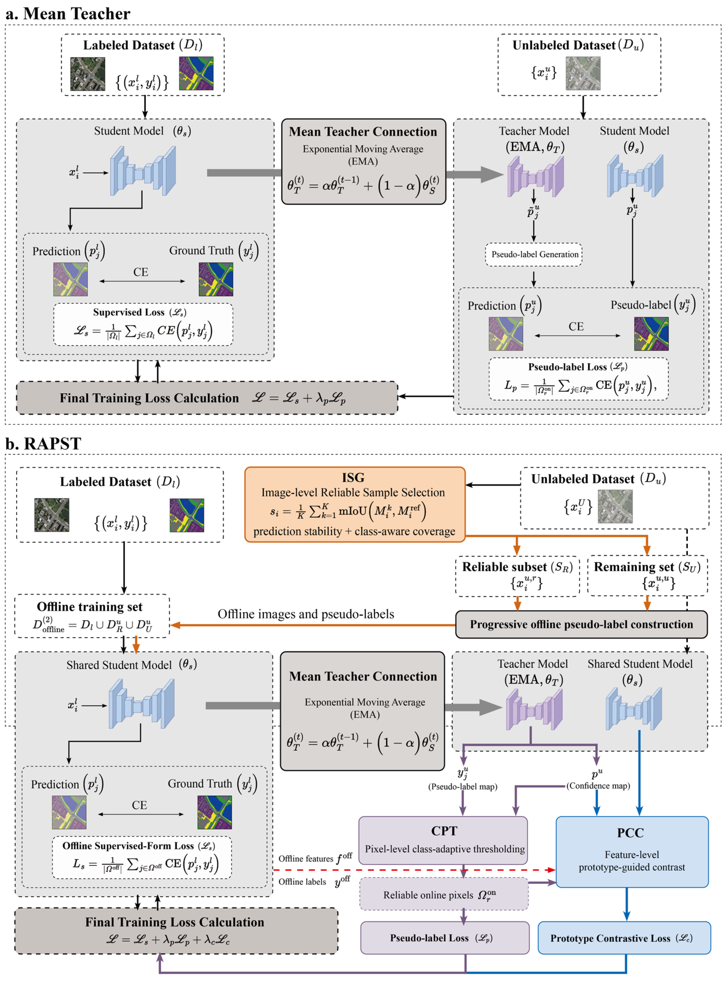
The Mean Teacher framework consists of a student model and a teacher model parameterized by ${\theta }_s$ and ${\theta }_t$, respectively, as shown in Figure 1a. The student is optimized by backpropagation, while the teacher is updated using the exponential moving average of the student parameters:

$${\theta }_t^{\left(t\right)}=\alpha {\theta }_t^{\left(t-1\right)}+\left(1-\alpha \right){\theta }_s^{\left(t\right)}.$$

(8)

where $t$ denotes the training step and $\alpha$ is the EMA decay coefficient.

Figure 1. Overall framework of RAPST. (a) Mean Teacher baseline. (b) RAPST with ISG-based offline supervision, CPT-based online pseudo-label filtering, and PCC-based feature learning.

For an unlabeled image $x^u$, the teacher produces a class probability map:

$$p^u=f_{{\theta }_t}\left(x^u\right),$$

(9)

and the pseudo-label of pixel $j$ is as follows:

$$y_j^u=\arg \underset{c\in \left\{0,\dots ,C-1\right\}}{\mathrm{m}\mathrm{a}\mathrm{x}}{p}_{j,c}^u,$$

(10)

where $p_{j,c}^u$ denotes the predicted probability for class $c$.

RAPST uses these predictions in two ways. In the offline stream, ISG selects stable images while preserving class coverage and constructs $D_{\mathrm{o}\mathrm{f}\mathrm{f}\mathrm{l}\mathrm{i}\mathrm{n}\mathrm{e}}$ for reliable segmentation supervision. In the online stream, the complete unlabeled set $D_u$ is retained, and CPT selects reliable pixels using class-adaptive thresholds. Both streams share the student network, while PCC uses their reliable feature–label pairs to improve class separation, as shown in Figure 1b.

The total training objective is as follows:

$$\mathcal{L}={\mathcal{L}}_s+{\lambda }_p{\mathcal{L}}_p+{\lambda }_c{\mathcal{L}}_c,$$

(11)

where ${\mathcal{L}}_s$, ${\mathcal{L}}_p$, and ${\mathcal{L}}_c$ denote the offline segmentation loss, online pseudo-label loss, and feature-level contrastive loss, respectively.

For an offline batch, the segmentation loss is as follows:

$${\mathcal{L}}_s={\displaystyle \frac{1}{\mid {\mathsf{\Omega }}^{\mathrm{o}\mathrm{f}\mathrm{f}}\mid }}\sum _{j\in {\mathsf{\Omega }}^{\mathrm{o}\mathrm{f}\mathrm{f}}}\mathrm{C}\mathrm{E}\left(p_j^l,y_j^l\right),$$

(12)

where ${\mathsf{\Omega }}^{\mathrm{o}\mathrm{f}\mathrm{f}}$ denotes the valid pixels in the offline batch, and $y_j^l$ is either a ground-truth label or an ISG-generated offline pseudo-label.

For the online stream, the pseudo-label loss is as follows:

$${\mathcal{L}}_p={\displaystyle \frac{1}{\mid {\mathsf{\Omega }}_r^{\mathrm{o}\mathrm{n}}\mid }}\sum _{j\in {\mathsf{\Omega }}_r^{\mathrm{o}\mathrm{n}}}\mathrm{C}\mathrm{E}\left(p_j^u,y_j^u\right),$$

(13)

where ${\mathsf{\Omega }}_r^{\mathrm{o}\mathrm{n}}$ denotes the reliable online pixels selected by CPT.

The offline and online streams provide complementary segmentation supervision, while PCC further constrains their shared feature representation.

3.3. ISG: Class-Aware Image Stability Gate

The offline stream requires pseudo-labeled images that are both reliable and representative of different land-cover classes. ISG therefore combines multi-checkpoint prediction stability with class-aware image selection.

During the Mean Teacher warm-up stage, intermediate EMA checkpoints are saved at predefined training stages, and the final scheduled EMA checkpoint is used as the stability reference. For an unlabeled image $x_i^u$, its stability score is defined as

$$s_i={\displaystyle \frac{1}{K}}{\displaystyle \sum _{k=1}^K}\mathrm{mIoU}\left(M_i^k,M_i^{\mathrm{r}\mathrm{e}\mathrm{f}}\right).$$

(14)

where $M_i^k$ and $M_i^{\mathrm{r}\mathrm{e}\mathrm{f}}$ are the masks predicted by the $k$-th intermediate and reference checkpoints, respectively. The mask-to-mask mIoU includes all semantic classes, including background; classes absent from both masks are omitted, while a class appearing in only one mask has an IoU of zero.

Pure stability ranking may underrepresent classes occupying fewer pixels. ISG therefore introduces a class-aware constraint based on the predicted pixel mass of the reference masks. Let $a_{i,c}$ denote the number of pixels of class $c$ in image $i$, and $A_c$ its total pixel mass over the unlabeled set. The class-specific coverage target $Q_c$ and selection score $r_{i,c}$ are defined as

$$a_{i,c}=\mid \left\{p:M_{i,p}^{\mathrm{r}\mathrm{e}\mathrm{f}}=c\right\}\mid , A_c=\sum _i{a}_{i,c}, Q_c=\eta A_c, r_{i,c}=s_i{\displaystyle \frac{a_{i,c}}{HW}}.$$

(15)

Classes are processed from rare to frequent according to $A_c$. For each class, images are selected in descending order of $r_{i,c}$ until its accumulated pixel coverage reaches $Q_c$ or the overall selection budget is exhausted. A multi-class image contributes simultaneously to all classes it contains; classes absent from the reference predictions are skipped. Ties are resolved by higher stability and then sample order. Background is excluded from class-aware coverage for Vaihingen and Potsdam, whereas all semantic classes are considered for WHDLD.

Let $N_u$ denote the number of unlabeled images and $\rho$ the retention ratio. The number of reliable images is

$$N_r=⌊\rho N_u⌋,$$

(16)

If the class-specific targets are satisfied before $N_r$ images are selected, the remaining budget is filled in descending order of stability. Thus, class information adjusts the composition of the reliable offline subset without replacing stability as the primary reliability criterion. The values of $K$, $\rho$, and $\eta$ are given in Section 4.1.2.

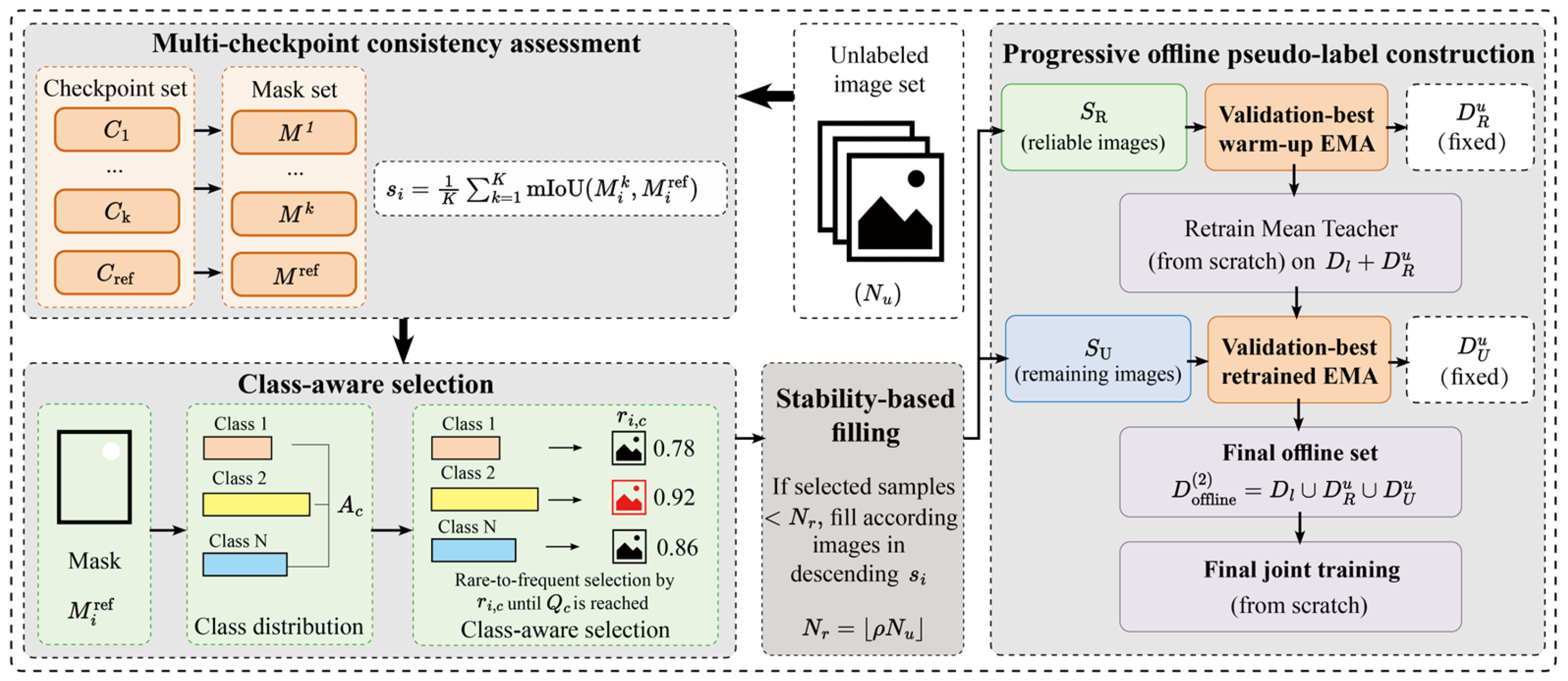
The validation-best warm-up EMA teacher generates fixed pseudo-labels for the selected reliable images, forming $D_R^u$. A new Mean Teacher is then trained from scratch using $D_{\mathrm{o}\mathrm{f}\mathrm{f}\mathrm{l}\mathrm{i}\mathrm{n}\mathrm{e}}^1$, and its validation-best EMA teacher generates pseudo-labels for the remaining images to form $D_U^u$ and $D_{\mathrm{o}\mathrm{f}\mathrm{f}\mathrm{l}\mathrm{i}\mathrm{n}\mathrm{e}}^2$. Final joint training again starts from scratch and uses $D_{\mathrm{o}\mathrm{f}\mathrm{f}\mathrm{l}\mathrm{i}\mathrm{n}\mathrm{e}}^2$ as fixed offline supervision, while the complete $D_u$ provides dynamic online supervision. Offline pseudo-labels are not refreshed after generation. The complete progressive ISG workflow is illustrated in Figure 2.

Figure 2. Progressive ISG workflow, including multi-checkpoint stability assessment, class-aware reliable-image selection, and progressive offline pseudo-label construction.

3.4. CPT: EMA-Smoothed Class-Adaptive Pseudo-Label Thresholding

ISG initially restricts offline supervision to the selected reliable images, whereas the online stream retains the complete unlabeled set throughout training. However, a fixed confidence threshold tends to favor large and easily recognized land-cover classes, while predictions for cars, difficult vegetation regions, and object boundaries are more frequently discarded. CPT addresses this imbalance by adapting the online selection threshold to the pseudo-label availability of each class.

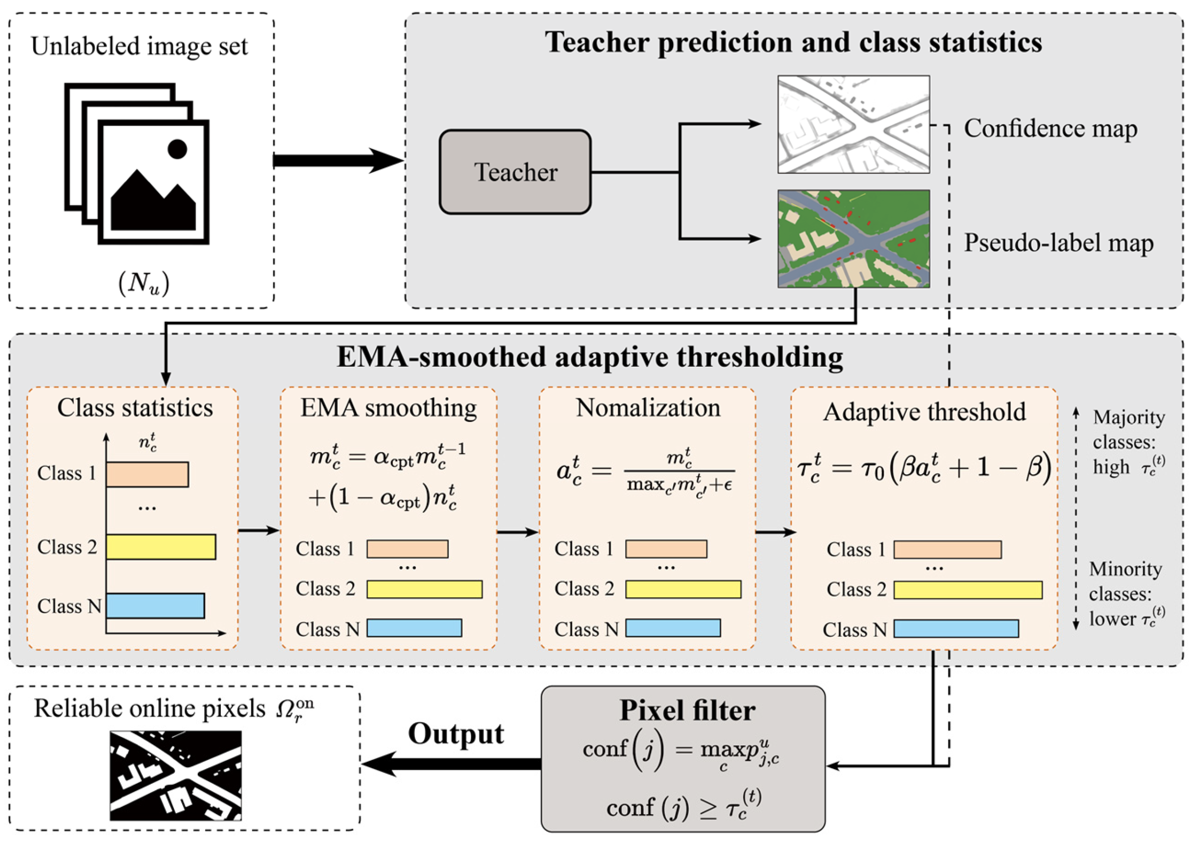
Because class-wise pseudo-label counts can fluctuate across mini-batches, CPT first smooths them using an exponential moving average. Let $n_c^{\left(t\right)}$ denote the number of pixels predicted as class $c$ in the current online batch at training step $t$. The smoothed statistic is defined as follows:

$$m_c^{\left(t\right)}={\alpha }_{\mathrm{c}\mathrm{p}\mathrm{t}}{m}_c^{\left(t-1\right)}+\left(1-{\alpha }_{\mathrm{c}\mathrm{p}\mathrm{t}}\right)n_c^{\left(t\right)}.$$

(17)

The smoothed count is then normalized by the maximum across classes, using the most represented class as a relative reference while avoiding dependence on the absolute batch pixel count:

$$a_c^{\left(t\right)}={\displaystyle \frac{m_c^{\left(t\right)}}{\underset{c^{\prime }\in \left\{0,\dots ,C-1\right\}}{\mathrm{m}\mathrm{a}\mathrm{x}}{m}_{c^{\prime }}^{\left(t\right)}+ϵ}},$$

(18)

where $ϵ$ is a small constant used to avoid division by zero.

Based on the normalized statistic, CPT assigns a dynamic confidence threshold to each class:

$${\tau }_c^{\left(t\right)}={\tau }_0\left(\beta a_c^{\left(t\right)}+1-\beta \right),$$

(19)

where ${\tau }_0$ denotes the base threshold and $\beta$ controls the adjustment amplitude. Classes with abundant pseudo-labels retain thresholds close to ${\tau }_0$, whereas classes receiving less online supervision are assigned lower thresholds. This allows difficult and sparsely distributed classes to contribute more useful pixels without applying uniformly relaxed filtering to all categories.

For an unlabeled pixel $j$ whose predicted class is $c$, its confidence is defined as follows:

$$\mathrm{c}\mathrm{o}\mathrm{n}\mathrm{f}\left(j\right)=\underset{c\in \left\{0,\dots ,C-1\right\}}{\mathrm{m}\mathrm{a}\mathrm{x}}{p}_{j,c}^u.$$

(20)

The pixel is retained when

$$\mathrm{c}\mathrm{o}\mathrm{n}\mathrm{f}\left(j\right)\ge {\tau }_c^{\left(t\right)}.$$

(21)

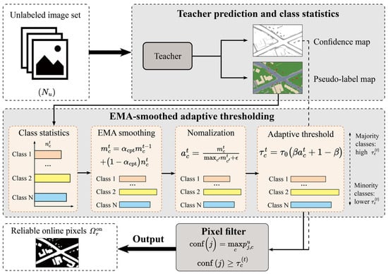
Pixels satisfying Equation (21) form the reliable online pixel set ${\mathsf{\Omega }}_r^{\mathrm{o}\mathrm{n}}$. They contribute to the online pseudo-label loss and provide reliable online feature–label pairs for PCC. CPT thus preserves the broad coverage of the complete unlabeled set while reducing the class bias introduced by fixed-threshold selection. The complete CPT filtering process is illustrated in Figure 3.

Figure 3. CPT-based class-adaptive pseudo-label filtering in the online supervision stream.

3.5. PCC: Reliability-Aware Prototype-Guided Category Contrast

Reliable pixel selection improves supervision quality, but visually similar remote sensing classes may still overlap in the shared feature space. Low vegetation and trees often exhibit similar spectral and textural characteristics, while buildings and impervious surfaces may share similar appearance and spatial patterns. PCC therefore combines reliable features from both supervision streams to construct class references and uses informative online pixels to improve class separation.

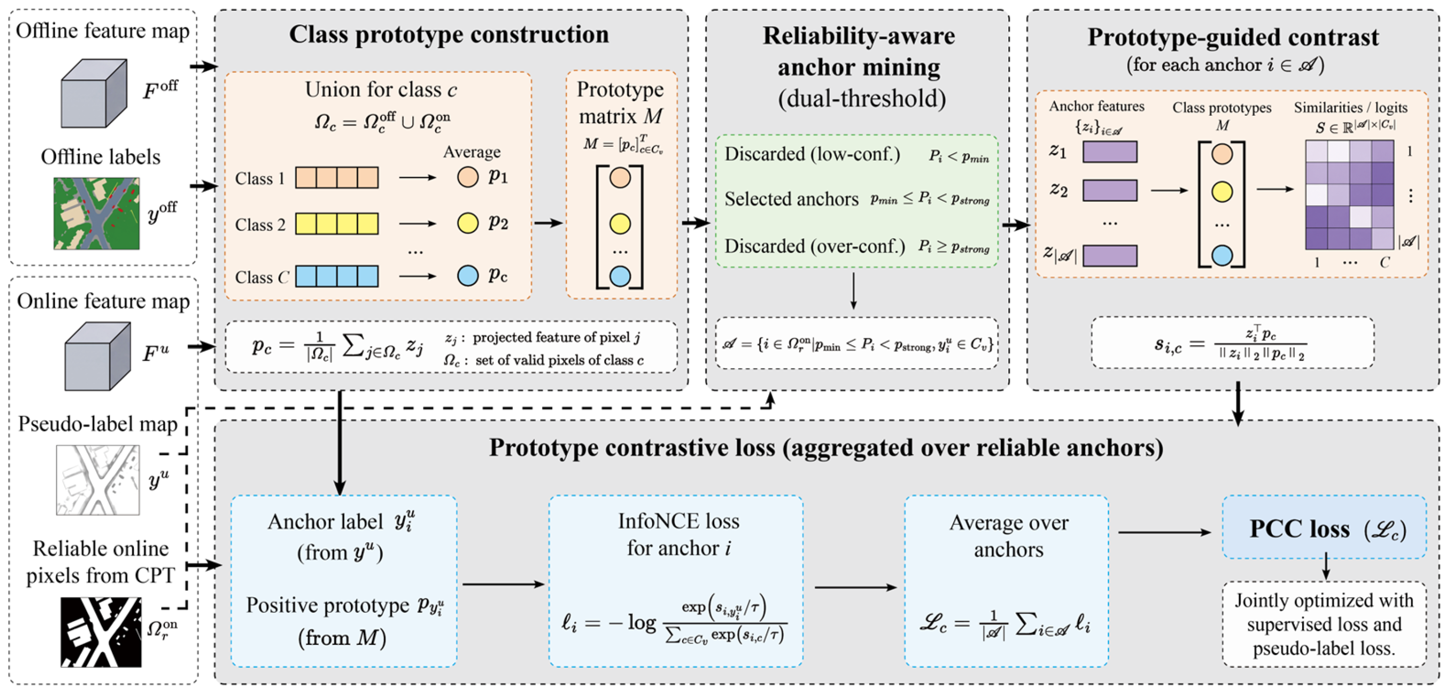
Let $z_j\in {\mathbb{R}}^d$ denote the projected feature of pixel $j$. For class $c$, the reliable offline and online pixel sets are defined as follows:

$${\mathsf{\Omega }}_c^{\mathrm{o}\mathrm{f}\mathrm{f}}=\left\{j\mid y_j^{\mathrm{o}\mathrm{f}\mathrm{f}}=c\right\},{\mathsf{\Omega }}_c^{\mathrm{o}\mathrm{n}}=\left\{j\in {\mathsf{\Omega }}_r^{\mathrm{o}\mathrm{n}}\mid y_j^u=c\right\},$$

(22)

where $y_j^{\mathrm{o}\mathrm{f}\mathrm{f}}$ is either a ground-truth label or an ISG-generated offline pseudo-label. The joint reliable pixel set and the valid class set are as follows:

$${\mathsf{\Omega }}_c={\mathsf{\Omega }}_c^{\mathrm{o}\mathrm{f}\mathrm{f}}\cup {\mathsf{\Omega }}_c^{\mathrm{o}\mathrm{n}},{\mathcal{C}}_v=\left\{c\mid \mid {\mathsf{\Omega }}_c\mid >0\right\}.$$

(23)

For each valid class $c\in {\mathcal{C}}_v$, the class prototype is calculated as follows:

$$p_c={\displaystyle \frac{1}{∣{\mathsf{\Omega }}_c∣}}\sum _{j\in {\mathsf{\Omega }}_c}{z}_j,c\in {\mathcal{C}}_v,$$

(24)

where $p_c$ represents the prototype of class $c$ in the current iteration. The valid prototypes are stacked to form the prototype matrix:

$$M={\left[p_c\right]}_{c\in {\mathcal{C}}_v}^{\mathrm{T}}\in {\mathbb{R}}^{∣{\mathcal{C}}_v∣\times d},$$

(25)

where $d$ denotes the projected feature dimension. PCC uses batch-local prototypes only; classes without reliable pixels in the current mini-batch are omitted from ${\mathcal{C}}_v$, and no cross-batch prototype memory is maintained.

Not all reliable online pixels are equally informative for contrastive learning. Low-confidence predictions are more susceptible to pseudo-label noise, whereas highly confident pixels are typically already well aligned with their predicted classes and provide limited additional contrastive gradients. PCC therefore selects reliable yet non-saturated online pixels as contrastive anchors. Let $P_i$ denote the teacher confidence of online pixel $i$. The anchor set is defined as follows:

$$\mathcal{A}=\left\{i,\in {\mathsf{\Omega }}_r^{\mathrm{o}\mathrm{n}}\mid p_{\mathrm{m}\mathrm{i}\mathrm{n}}\le P_i<p_{\mathrm{s}\mathrm{t}\mathrm{r}\mathrm{o}\mathrm{n}\mathrm{g}} y_i^u\in {\mathcal{C}}_v\right\},$$

(26)

where $p_{\mathrm{m}\mathrm{i}\mathrm{n}}$ filters low-confidence predictions, while $p_{\mathrm{s}\mathrm{t}\mathrm{r}\mathrm{o}\mathrm{n}\mathrm{g}}$ restricts anchor selection to non-saturated pixels. Pixels above $p_{\mathrm{s}\mathrm{t}\mathrm{r}\mathrm{o}\mathrm{n}\mathrm{g}}$ remain available for segmentation supervision and prototype construction and are excluded only from contrastive anchoring.

For an anchor $i\in \mathcal{A}$, the cosine similarity between its feature and prototype $p_c$ is as follows:

$$s_{i,c}={\displaystyle \frac{z_i^T{p}_c}{\parallel z_i{\parallel }_2\parallel p_c{\parallel }_2}},c\in {\mathcal{C}}_v.$$

(27)

The prototype corresponding to $y_i^u$ is treated as the positive prototype, while the remaining valid prototypes serve as negatives. The contrastive loss for anchor $i$ is as follows:

$${\mathcal{l}}_i=-\log {\displaystyle \frac{\mathrm{e}\mathrm{x}\mathrm{p}\left(s_{i,y_i^u}/\tau \right)}{\sum _{c\in {\mathcal{C}}_v}\mathrm{e}\mathrm{x}\mathrm{p}\left(s_{i,c}/\tau \right)}},$$

(28)

where $\tau$ is the temperature coefficient. The PCC loss is as follows:

$${\mathcal{L}}_c={\displaystyle \frac{1}{\mid \mathcal{A}\mid }}\sum _{i\in A}{\mathcal{l}}_i.$$

(29)

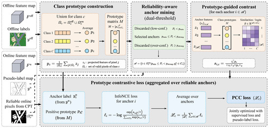
If fewer than two valid class prototypes or no valid anchors are available, ${\mathcal{L}}_c$ is set to zero for the current iteration. By combining reliable information from both streams with informative online anchors, PCC improves the discriminability of the shared feature space. The PCC workflow is illustrated in Figure 4.

Figure 4. PCC with cross-stream prototype construction and online anchor contrast.

4. Experiments and Results

4.1. Experimental Setup

4.1.1. Datasets

This paper evaluates the effectiveness of the proposed method on three public remote sensing semantic segmentation datasets, namely ISPRS Vaihingen, ISPRS Potsdam, and WHDLD.

The ISPRS Vaihingen dataset contains high-resolution aerial images of Vaihingen, Germany, with a spatial resolution of approximately 9 cm. The ISPRS Potsdam dataset contains aerial images of Potsdam, Germany, with a spatial resolution of approximately 5 cm. Both datasets contain six semantic classes: impervious surfaces, buildings, low vegetation, trees, cars, and background. IRRG imagery and nDSM are used as four-channel inputs. WHDLD contains 4940 pre-cropped satellite image tiles with a spatial resolution of 2 m and six classes: building, road, pavement, vegetation, bare soil, and water. RGB imagery is used as input.

To simulate different annotation-cost settings, a proportion of the training samples is selected as labeled data and the remainder is treated as unlabeled data. Four annotation ratios are used: 1/32, 1/16, 1/8, and 1/4. Dataset details are summarized in Table 1. Detailed training/evaluation identifiers, patch construction, preprocessing, split rules, and exact labeled/unlabeled sample numbers are provided in Appendix A.

Table 1. Basic dataset information and semi-supervised split settings.

Dataset	Training Samples	Evaluation Samples	Input Channels	Number of Classes	Annotation Ratios
ISPRS Vaihingen	344 patches	17 areas	4 (IRRG + nDSM)	6	1/32, 1/16, 1/8, 1/4
ISPRS Potsdam	3456 patches	14 tiles	4 (IRRG + nDSM)	6	1/32, 1/16, 1/8, 1/4
WHDLD	3952 images	988 images	3 (RGB)	6	1/32, 1/16, 1/8, 1/4

Note: For the ISPRS datasets, evaluation follows the no Boundary setting, where pixels labeled 255 in the eroded ground truth are ignored.

4.1.2. Implementation Details

All methods are re-implemented in a unified codebase using the same UNet backbone. For Vaihingen and Potsdam, all methods use four-channel IRRG + nDSM inputs; the first convolutional layer is directly constructed with four input channels and trained from scratch using Kaiming initialization. WHDLD uses the native three-channel RGB input. Unless otherwise stated, all methods use the same data splits, optimization settings, data augmentation, training schedule, early stopping criterion, and model-selection criterion. Method-specific hyperparameters are adopted from the corresponding original publications without re-tuning on our datasets. The checkpoint with the highest validation mIoU is selected for evaluation.

Models are optimized with SGD and PolyLR. ISG constructs the offline pseudo-labeled set from the warm-up checkpoints; during joint training, the EMA teacher supplies online predictions, CPT filters their pixels, and PCC constrains the shared feature space. Hyperparameters remain fixed across annotation ratios on each dataset. The implementation details and hyperparameter settings are summarized in Table 2.

Table 2. Implementation details and hyperparameter configuration.

Category	Parameter	Value
Environment	GPU	NVIDIA GeForce RTX 4060 Ti (16 GB)
	PyTorch/CUDA	PyTorch 2.5.1/CUDA 12.4
Network & Optimization	Network	UNet
	Optimizer	SGD, momentum = 0.9, Nesterov
	Weight Decay	$1\times {10}^{-4}$
	Initial LR	0.01
	LR Schedule	PolyLR, power = 0.9
Training Strategy	Batch Size	8 (4 Offline + 4 Online)
	Max Epochs	$100$
	Iterations	Vaihingen: 200; Potsdam: 400; WHDLD: 500
	Augmentation	Horizontal/vertical flip + 90° rotations
	Early Stopping	Grace period = 10; Patience = 12; min_delta = 0.0005
	Model Selection	Best validation mIoU
RAPST Hyperparameters	Base Threshold/Loss Weights	${\tau }_0=0.95$; ${\lambda }_p=1.0$, ${\lambda }_c=1.0$ for Vaihingen/Potsdam, ${\lambda }_c=0.5$ for WHDLD
	Teacher EMA	$\alpha =0.999$
	ISG	$K=2$; $\rho =0.5$; η $=0.01$ for Vaihingen/Potsdam, η $=0.05$ for WHDLD
	CPT	${\alpha }_{\mathrm{cpt}}=0.9$; $\beta =0.1$
	PCC	Dim = $64$; $\tau =0.05$
	Confidence Bounds	$p_{\mathrm{m}\mathrm{i}\mathrm{n}}=0.5$; $p_{\mathrm{strong}}=0.98$

4.1.3. Evaluation Metrics

Per-class F1 score and mean Intersection-over-Union (mIoU) are used as the main evaluation metrics. For the ISPRS Vaihingen and Potsdam datasets, evaluation is performed on the five relevant land-cover classes—impervious surfaces, buildings, low vegetation, trees, and cars. Following the ISPRS 2D Semantic Labeling benchmark convention, background is excluded from the class-averaged metrics. The same evaluation protocol is applied to all compared methods. For WHDLD, which contains six semantic land-cover categories without a separate background class, all six classes are included in the evaluation.

For class $c$, the F1 score is defined as follows:

$$F{1}_c={\displaystyle \frac{2T{P}_c}{2T{P}_c+F{P}_c+F{N}_c}},$$

(30)

where $T{P}_c$, $F{P}_c$, and $F{N}_c$ denote the true positives, false positives, and false negatives for class $c$, respectively.

For overall segmentation performance, this paper uses mIoU for evaluation. The IoU of class $c$ is defined as follows:

$$Io{U}_c={\displaystyle \frac{T{P}_c}{T{P}_c+F{P}_c+F{N}_c}}.$$

(31)

mIoU is the mean IoU over the evaluated semantic classes:

$$\mathrm{m}\mathrm{I}\mathrm{o}\mathrm{U}={\displaystyle \frac{1}{\mid {\mathcal{C}}_{\mathrm{e}\mathrm{v}\mathrm{a}\mathrm{l}}\mid }}\sum _{c\in {\mathcal{C}}_{\mathrm{e}\mathrm{v}\mathrm{a}\mathrm{l}}}{\mathrm{I}\mathrm{o}\mathrm{U}}_c,$$

(32)

where ${\mathcal{C}}_{\mathrm{e}\mathrm{v}\mathrm{a}\mathrm{l}}$ contains the five foreground classes for Vaihingen and Potsdam and all six semantic classes for WHDLD.

4.2. Comparison with Existing Methods

To evaluate the effectiveness of RAPST, we compare it with the supervised-only baseline OnlySup and representative semi-supervised methods, including Mean Teacher (2017) [4], ST++ (2022) [5], CPS (2021) [15], UniMatch (2023) [16], MUCA (2025) [47], and DWL (2024) [7], on the ISPRS Vaihingen, ISPRS Potsdam, and WHDLD datasets. All methods use the same data splits, dataset-specific input formats, segmentation network, and evaluation metrics. The annotation ratios of 1/32, 1/16, 1/8, and 1/4 are evaluated, with the remaining training samples used as unlabeled data.

As shown in Table 3, RAPST achieves the highest mIoU under the 1/32, 1/16, and 1/8 annotation ratios on the Vaihingen dataset, while remaining competitive under the 1/4 setting. Compared with OnlySup, RAPST improves mIoU by 3.96–6.02 percentage points, with the largest gain obtained under the 1/32 setting. Under the first three annotation ratios, RAPST exceeds the strongest competing method by 0.42–0.94 percentage points, whereas ST++ achieves the highest result under the 1/4 setting. These results show that RAPST maintains strong performance across different levels of labeled supervision, with particularly clear gains under severe label scarcity.

Table 3. mIoU comparison results of different methods on the ISPRS Vaihingen dataset (%).

Method	1/32	1/16	1/8	1/4
OnlySup	60.92	67.24	68.39	71.03
Mean Teacher	64.35	69.96	71.86	73.71
ST++	66.52	71.74	73.07	75.59
CPS	64.49	70.51	70.68	71.43
UniMatch	63.45	69.98	70.67	74.37
DWL	65.15	68.87	70.98	74.24
MUCA	63.00	68.96	69.33	71.77
RAPST (Ours)	66.94	72.68	73.84	74.99

As shown in Table 4, RAPST achieves the highest mIoU under all four annotation ratios on the Potsdam dataset. Compared with OnlySup, RAPST improves mIoU by 1.95–6.08 percentage points, with the largest gain again obtained under the 1/32 setting. Compared with the strongest competing method at each annotation ratio, RAPST achieves improvements of 0.39–0.68 percentage points. The consistent results on Potsdam further demonstrate the effectiveness of RAPST across different levels of labeled supervision.

Table 4. mIoU comparison results of different methods on the ISPRS Potsdam dataset (%).

Method	1/32	1/16	1/8	1/4
OnlySup	74.02	77.13	77.94	79.83
Mean Teacher	77.30	78.52	79.52	80.94
ST++	79.42	79.37	80.28	81.36
CPS	77.32	78.56	78.82	81.02
UniMatch	78.58	79.68	79.45	80.48
DWL	76.21	78.34	79.83	80.33
MUCA	73.84	76.53	78.19	79.21
RAPST (Ours)	80.10	80.24	80.67	81.78

As shown in Table 5, RAPST achieves the highest mIoU under the 1/32, 1/16, and 1/8 annotation ratios on the WHDLD dataset, while remaining competitive under the 1/4 setting. Compared with OnlySup, RAPST improves mIoU by 0.33–3.47 percentage points, with the largest gain again obtained under the 1/32 setting. Under the first three annotation ratios, RAPST exceeds the strongest competing result by 0.05–0.65 percentage points, whereas DWL achieves the highest result under the 1/4 setting. These results further support the effectiveness of RAPST on RGB satellite imagery with substantially different spatial resolution and scene characteristics from the two ISPRS benchmarks.

Table 5. mIoU comparison results of different methods on the WHDLD dataset (%).

Method	1/32	1/16	1/8	1/4
OnlySup	54.09	56.68	58.70	60.39
Mean Teacher	55.46	57.00	58.81	60.44
ST++	56.91	57.37	59.24	60.47
CPS	55.75	56.64	58.83	59.61
UniMatch	55.90	57.23	59.30	60.52
DWL	54.53	56.74	59.25	60.91
MUCA	54.94	57.47	56.68	60.34
RAPST (Ours)	57.56	57.71	59.35	60.72

Across the three datasets, RAPST achieves the highest mIoU in 10 of the 12 dataset–annotation settings. In particular, the largest improvements over OnlySup occur under the 1/32 setting on all three datasets, indicating that the framework is especially effective under severe label scarcity. The two exceptions occur under the 1/4 setting on Vaihingen and WHDLD, where RAPST remains close to the strongest competing method. Overall, these results support the consistent effectiveness of RAPST across different datasets and annotation ratios. The contribution of each component is examined in the following ablation studies.

4.3. Ablation Studies

To identify the contributions of the individual components in RAPST, we evaluate ISG, CPT, and PCC separately and in representative combinations on the ISPRS Vaihingen, ISPRS Potsdam, and WHDLD datasets. OnlySup and Mean Teacher are used as the supervised and semi-supervised baselines, respectively. In addition, to further examine whether the component contributions remain stable under a stricter early-stopping condition, we conduct an additional experiment on Vaihingen using training seed 3047 and a patience of 8, compared with training seed 2023 and patience = 12 in the standard setting.

As shown in Table 6, all three components improve upon the Mean Teacher baseline on Vaihingen, with ISG providing the largest individual gain. Among the two-component configurations, ISG + PCC achieves the highest mIoU of 72.08%, while the complete RAPST further improves the result to 72.68%, exceeding Mean Teacher by 3.08 percentage points. The class-wise F1 results also show improvements across all five foreground classes compared with Mean Teacher.

Table 6. Ablation results of RAPST under the 1/16 annotation ratio on the ISPRS Vaihingen dataset (%).

Group	ISG	CPT	PCC	F1_Imp	F1_Bld	F1_Low	F1_Tre	F1_Car	mIoU
OnlySup				86.36	90.24	78.59	86.10	54.84	67.27
Mean Teacher				87.24	91.12	78.83	87.41	61.37	69.60
ISG	✓			88.12	92.77	81.39	88.58	61.53	71.57
CPT		✓		87.36	91.82	80.11	87.67	64.34	70.95
PCC			✓	87.87	91.58	80.53	87.56	61.37	70.48
ISG + CPT	✓	✓		88.16	92.80	80.94	88.28	62.34	71.54
CPT + PCC		✓	✓	87.93	91.99	80.56	87.76	65.73	71.64
ISG + PCC	✓		✓	88.14	92.66	81.08	88.31	64.91	72.08
RAPST (Ours)	✓	✓	✓	88.30	92.30	81.81	88.53	66.67	72.68

The additional Vaihingen results in Table 7 show a similar overall pattern under seed 3047 and the stricter early-stopping setting. ISG again provides the largest individual improvement, increasing mIoU from 69.91% to 71.42%. Among the two-component configurations, CPT + PCC achieves the highest mIoU of 71.74%, while the complete RAPST reaches 71.89%, outperforming Mean Teacher by 1.98 percentage points. Together with the standard results in Table 6, these results show that the overall component contributions remain consistent across the two training settings.

Table 7. Additional robustness ablation results of RAPST on the ISPRS Vaihingen dataset under the 1/16 annotation ratio using seed 3047 and stricter early stopping (patience = 8) (%).

Group	ISG	CPT	PCC	F1_Imp	F1_Bld	F1_Low	F1_Tre	F1_Car	mIoU
OnlySup				86.36	90.19	77.59	85.87	54.99	66.93
Mean Teacher				87.09	91.16	80.28	87.68	60.67	69.91
ISG	✓			87.76	91.88	80.88	88.07	64.24	71.42
CPT		✓		88.06	91.95	79.92	87.61	62.14	70.67
PCC			✓	87.52	91.82	80.02	87.61	63.81	70.84
ISG + CPT	✓	✓		88.38	92.52	81.63	87.91	59.59	71.02
CPT + PCC		✓	✓	87.34	91.95	80.13	87.43	68.04	71.74
ISG + PCC	✓		✓	87.79	91.91	80.92	88.10	64.31	71.47
RAPST (Ours)	✓	✓	✓	87.87	91.94	81.36	88.44	64.99	71.89

As shown in Table 8, a similar pattern is observed on Potsdam. ISG again provides the largest individual improvement, increasing mIoU from 78.00% to 79.27%. ISG + PCC achieves the best two-component result of 79.92%, and the complete RAPST reaches the highest mIoU of 80.10%, outperforming Mean Teacher by 2.10 percentage points. The class-wise F1 results likewise show consistent improvements across the evaluated foreground classes.

Table 8. Ablation results of RAPST under the 1/32 annotation ratio on the ISPRS Potsdam dataset (%).

Group	ISG	CPT	PCC	F1_Imp	F1_Bld	F1_Low	F1_Tre	F1_Car	mIoU
OnlySup				87.94	93.05	79.44	77.20	87.55	74.42
Mean Teacher				89.15	94.44	81.54	81.55	90.36	78.00
ISG	✓			89.87	94.66	83.64	82.88	90.26	79.27
CPT		✓		89.42	94.60	81.69	81.72	90.05	78.13
PCC			✓	88.82	94.89	81.73	81.97	90.48	78.26
ISG + CPT	✓	✓		90.32	94.57	83.43	83.10	90.84	79.58
CPT + PCC		✓	✓	89.52	94.59	82.47	81.74	90.63	78.58
ISG + PCC	✓		✓	90.50	94.93	83.32	83.18	91.30	79.92
RAPST (Ours)	✓	✓	✓	90.68	94.77	83.54	83.01	91.78	80.10

As shown in Table 9, the WHDLD results further support these observations. ISG provides the largest individual improvement over Mean Teacher, increasing mIoU from 55.46% to 57.17%. Among the two-component configurations, CPT + PCC achieves the highest mIoU of 57.50%, while the complete RAPST reaches the highest overall mIoU of 57.56%, outperforming Mean Teacher by 2.10 percentage points.

Table 9. Ablation results of RAPST under the 1/32 annotation ratio on the WHDLD dataset (%).

Group	ISG	CPT	PCC	F1_Bld	F1_Road	F1_Pav	F1_Veg	F1_Bare	F1_Water	mIoU
OnlySup				65.20	59.40	49.26	86.76	50.42	95.24	54.09
Mean Teacher				64.84	63.63	52.44	86.35	50.86	96.10	55.46
ISG	✓			66.78	66.17	54.06	87.29	52.87	96.38	57.17
CPT		✓		65.99	66.54	52.75	85.93	49.90	96.48	56.12
PCC			✓	67.50	68.06	52.73	87.11	50.48	96.48	57.08
ISG + CPT	✓	✓		66.93	66.88	54.30	87.32	53.18	96.46	57.45
CPT + PCC		✓	✓	67.78	68.49	54.13	87.44	50.15	96.58	57.50
ISG + PCC	✓		✓	66.44	66.69	54.58	87.29	53.09	96.08	57.22
RAPST (Ours)	✓	✓	✓	67.18	67.43	54.55	87.49	52.65	96.35	57.56

Overall, the ablation results exhibit a consistent pattern across the three datasets: ISG provides the strongest individual contribution, while the complete RAPST achieves the highest overall mIoU in all reported ablation settings. The two Vaihingen runs further show that the overall component contributions remain consistent across different training settings, including the stricter early-stopping setting used with seed 3047. These results support the complementary roles of ISG, CPT, and PCC. Section 4.4 further examines whether each component produces its intended effect.

4.4. Mechanism Validation of RAPST

The ablation results in Section 4.3 establish the contributions of ISG, CPT, and PCC. This section further examines whether the observed performance gains are consistent with the mechanisms for which these components were designed. All mechanism-level analyses are conducted on the ISPRS Potsdam dataset under the 1/32 annotation ratio. We first examine whether the ISG stability score reflects offline pseudo-label quality, then evaluate the precision–coverage trade-off introduced by CPT, and finally assess whether PCC improves feature-space separability. Qualitative comparisons on both datasets illustrate how these effects appear in the final segmentation results.

4.4.1. Stability–Quality Analysis of ISG

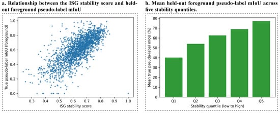
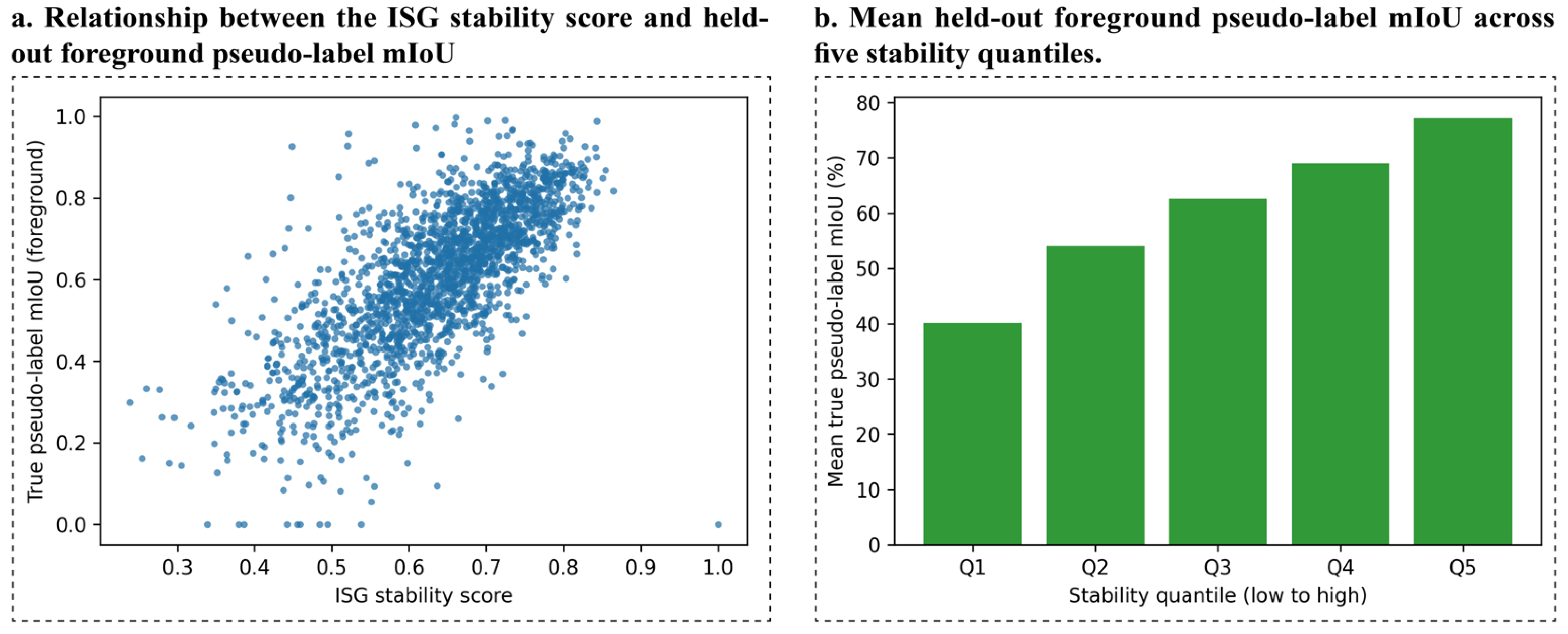
To determine whether the ISG stability score can identify reliable samples for offline pseudo-labeling, we compare the stability score of each unlabeled image with its foreground pseudo-label mIoU. The pseudo-label mIoU is computed using held-out ground-truth annotations solely for evaluation and does not participate in model training or sample selection.

As shown in Figure 5a, the ISG stability score is positively correlated with foreground pseudo-label mIoU, with a Spearman correlation coefficient of 0.7497. Figure 5b shows the same trend across stability quantiles: the mean foreground pseudo-label mIoU increases from 40.16% in Q1 to 77.16% in Q5. These results indicate that prediction consistency across checkpoints provides an effective criterion for ranking unlabeled images during offline pseudo-label construction.

Figure 5. Relationship between prediction stability and pseudo-label quality on the ISPRS Potsdam dataset under the 1/32 annotation ratio. (a) Relationship between the ISG stability score and held-out foreground pseudo-label mIoU. (b) Mean held-out foreground pseudo-label mIoU across five stability quantiles, from Q1 (lowest stability) to Q5 (highest stability).

4.4.2. Precision–Coverage Analysis of CPT

To examine how CPT changes the online supervision available to difficult and sparsely distributed classes, we compare a fixed confidence threshold with CPT using teacher predictions from the complete unlabeled set. For each class, precision measures the correctness of the retained pseudo-labels, whereas coverage measures the proportion of class-specific teacher predictions retained for online training.

As shown in Table 10, CPT increases pseudo-label coverage for all five foreground classes by 0.97–5.56 percentage points, while precision decreases by only 0.31–1.46 percentage points. Larger coverage gains are observed for low vegetation, trees, and cars, indicating that CPT provides more online supervision for relatively difficult classes at a limited precision cost.

Table 10. Pseudo-label precision and coverage before and after applying CPT on the ISPRS Potsdam dataset under the 1/32 annotation ratio (%).

Class	Coverage: Fixed → CPT	Δ Coverage	Precision: Fixed → CPT	Δ Precision
Impervious surfaces	78.46 → 80.45	+1.99	96.76 → 96.38	−0.38
Building	91.21 → 92.18	+0.97	97.83 → 97.52	−0.31
Low vegetation	66.89 → 71.23	+4.34	93.12 → 91.66	−1.46
Tree	68.48 → 74.04	+5.56	95.31 → 94.24	−1.07
Car	86.58 → 91.75	+5.17	98.40 → 97.39	−1.01

Note: → indicates the change from the fixed-threshold setting to CPT; Δ is calculated as CPT − Fixed.

4.4.3. Feature-Space Separability Analysis of PCC

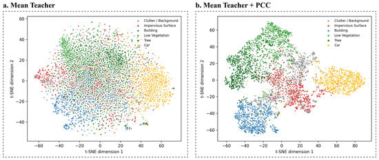
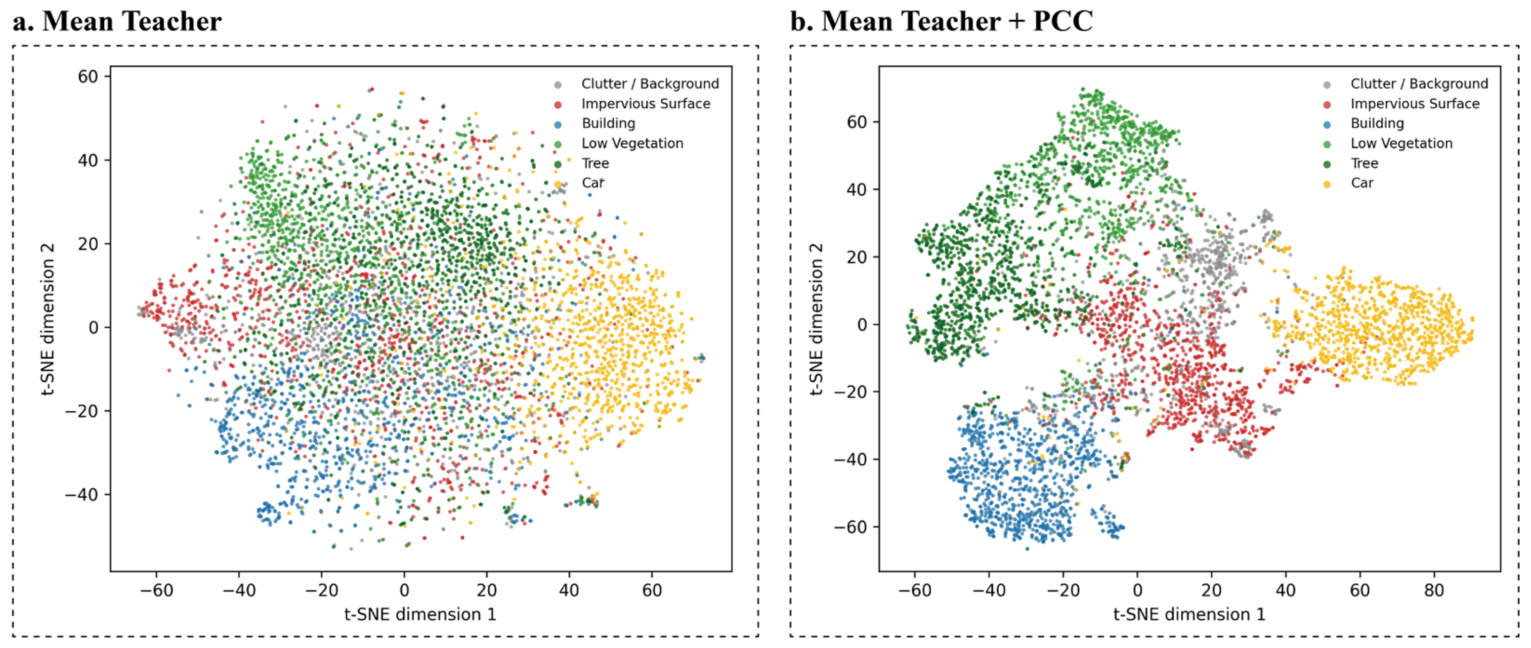
To determine whether PCC improves the shared feature representation, we compare Mean Teacher and Mean Teacher with PCC using both t-SNE visualization and quantitative cluster-validity metrics.

As shown in Figure 6a, the feature representations produced by Mean Teacher exhibit substantial overlap among several land-cover classes. After introducing PCC, Figure 6b shows more compact clusters and clearer separation between categories, suggesting improved feature discrimination.

Figure 6. t-SNE visualization of feature representations on the ISPRS Potsdam dataset under the 1/32 annotation ratio. (a) Mean Teacher. (b) Mean Teacher + PCC.

Because t-SNE provides only a two-dimensional qualitative view, the Silhouette Score and Davies–Bouldin Index are further calculated using the original high-dimensional features. A higher Silhouette Score indicates greater intra-class compactness and inter-class separation, whereas a lower Davies–Bouldin Index indicates better cluster separation.

As reported in Table 11, PCC increases the Silhouette Score from −0.0278 to 0.0953 and reduces the Davies–Bouldin Index from 8.3002 to 2.7313. The consistent improvements in both metrics agree with the t-SNE visualization and show that PCC produces more compact and better-separated class representations.

Table 11. Quantitative evaluation of feature-space separability on the ISPRS Potsdam dataset under the 1/32 annotation ratio.

Method	Silhouette Score	Davies–Bouldin Index
Mean Teacher	−0.0278	8.3002
Mean Teacher + PCC	0.0953	2.7313

4.4.4. Qualitative Segmentation Analysis

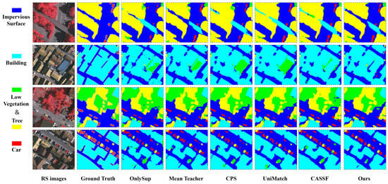
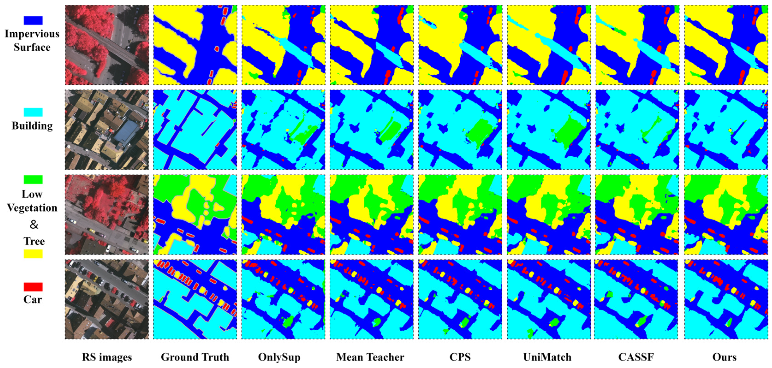
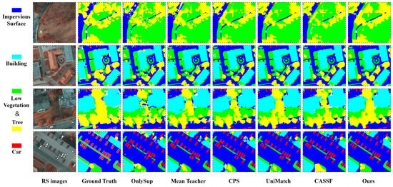
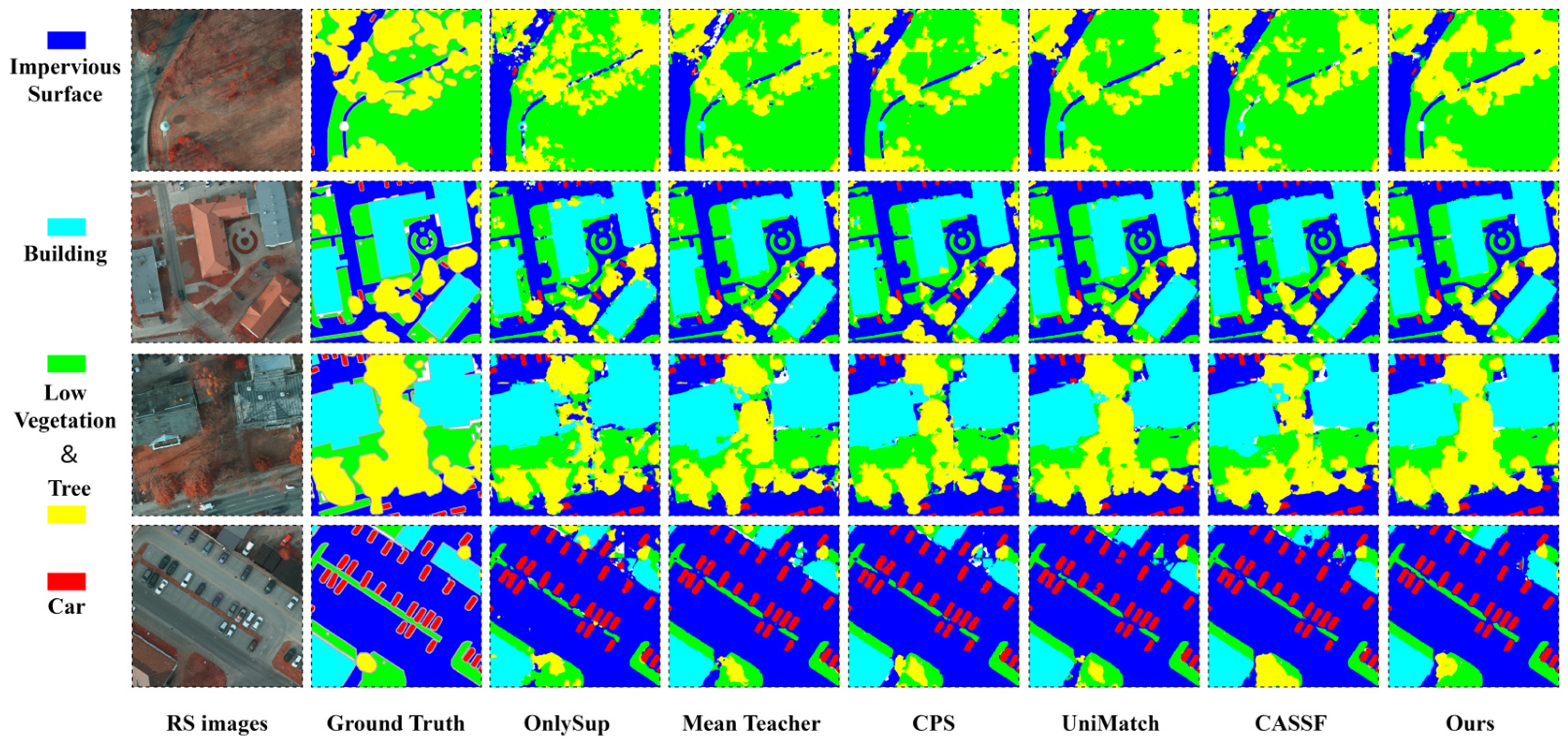
Figure 7 and Figure 8 compare the segmentation results of different methods on the ISPRS Vaihingen and Potsdam datasets. The selected scenes contain complex boundaries between buildings and impervious surfaces, visually similar vegetation classes, and small vehicle objects.

Figure 7. Category-oriented visual comparison results of different methods on the ISPRS Vaihingen dataset.

Figure 8. Category-oriented visual comparison results of different methods on the ISPRS Potsdam dataset.

OnlySup produces more fragmented regions, discontinuous boundaries, and local misclassifications because it relies solely on limited labeled data. The semi-supervised methods generally improve spatial continuity by incorporating unlabeled images, but errors remain around complex structures, vegetation transition regions, and small objects.

For buildings and impervious surfaces, RAPST produces more continuous regions and clearer structural boundaries in the selected examples. For low vegetation and trees, it reduces several misclassified areas caused by their similar spectral and spatial characteristics. For cars, RAPST preserves more small objects and produces more complete predictions in complex scenes, although minor boundary errors and object merging remain in some cases.

Overall, the qualitative results are consistent with the quantitative findings, showing clearer structural boundaries, reduced confusion between vegetation classes, and better preservation of small vehicles under limited annotation conditions.

4.5. Computational Efficiency

To evaluate the computational overhead of RAPST, Table 12 compares the efficiency of different methods on WHDLD under the 1/16 annotation setting. All methods are evaluated with 256 × 256 inputs and a batch size of 8 on an NVIDIA GeForce RTX 4060 Ti.

Table 12. Computational efficiency comparison of different methods on WHDLD under the 1/16 annotation setting.

Method	Params (M)	FLOPs (G/image)	Estimated Total Forward Compute (PFLOPs)	Peak Memory (GiB)	Train Time (h)	Inference Time (ms/Image)
OnlySup	7.77	27.51	3.08	0.93	0.42	2.40
Mean Teacher	7.77	27.51	16.51	1.68	1.00	2.40
ST++	7.77	27.51	48.61	1.68	2.93	2.40
CPS	7.77	27.51	29.05	3.11	1.72	2.40
UniMatch	7.77	27.51	33.02	3.03	2.05	2.40
MUCA	7.77	27.51	19.65	4.89	2.27	2.40
DWL	7.77	27.51	9.91	1.73	0.64	2.36
RAPST (Ours)	7.91	27.59	49.65	2.94	3.85	2.53

Note: Parameters, FLOPs, peak GPU memory, training time, and inference time are evaluated under the same hardware and input setting. Total compute accounts for all training stages included in each method.

As shown in Table 12, RAPST incurs a higher training cost than most competing methods, with its total computation being close to that of ST++. The additional overhead mainly arises from the multi-checkpoint stability evaluation, reliable-first retraining, progressive offline pseudo-label construction, and feature-level optimization introduced during training. Despite these additional stages, its peak GPU memory remains below that of several competing methods, indicating that the increased cost is primarily computational rather than memory-intensive.

At inference, the overhead remains limited. The parameter count, FLOPs, and inference latency of RAPST remain close to those of the common U-Net-based methods. Therefore, the additional computational cost of RAPST is concentrated mainly in training, while its deployment-time complexity remains comparable to the baseline segmentation network.

5. Discussion and Limitations

5.1. Discussion

The experimental results consistently show that RAPST is most beneficial under limited labeled supervision, with the largest gains over OnlySup appearing at the 1/32 annotation ratio across the three datasets. The mechanism analyses further show that prediction stability is associated with pseudo-label quality, CPT increases the participation of relatively difficult classes with limited precision loss, and PCC improves feature-space separability. These observations constitute the direct experimental evidence; their implications for the framework design are discussed below.

Compared with reliability-oriented self-training methods such as ST++ [5], which primarily improves pseudo-label quality through selective use of stable unlabeled images, RAPST maintains a separate online stream over the complete unlabeled set. Compared with class-aware methods such as CASSF [8], RAPST further separates image-level reliability control from online pixel-level adaptation. The consistent gains under low-label settings therefore suggest that reliability and data coverage are better treated as complementary objectives rather than being controlled by a single selection mechanism.

A similar distinction applies to prototype-based approaches [10,61]. Rather than constructing feature constraints from all available pseudo-labeled pixels, PCC restricts prototype construction and contrastive anchoring according to the reliability information supplied by the two supervision streams. The improved cluster separability observed in Section 4.4 supports the usefulness of this reliability-aware feature constraint, while the ablation results indicate that its effect is complementary to pseudo-label selection rather than sufficient on its own.

The benefit of RAPST is nevertheless expected to decrease when reliable supervision itself becomes difficult to establish. This may occur under substantial domain shift, extremely sparse class occurrence, or highly ambiguous boundaries, where stable predictions do not necessarily correspond to correct predictions and class prototypes may be supported by too few reliable pixels. The remaining boundary errors and object merging observed in the qualitative results are consistent with this scope. These cases suggest that stronger uncertainty estimation and spatial-structure modeling remain useful directions for further improvement.

5.2. Limitations

Although the three datasets cover both aerial and satellite imagery with different spatial resolutions and input modalities, broader validation across additional regions, sensors, and scene types is still needed. In addition, all experiments use U-Net as the common backbone for controlled comparison, so the architecture-level generalization of RAPST remains to be verified on Transformer- and state-space-based networks. RAPST also introduces additional training computation due to multi-checkpoint stability evaluation, progressive offline pseudo-label construction, and feature-level optimization, while its inference complexity remains close to that of the underlying segmentation network.

6. Conclusions

This study investigated the trade-off between pseudo-label reliability and unlabeled-data coverage in semi-supervised semantic segmentation of high-resolution remote sensing imagery. We proposed RAPST, a reliability-aware dual-stream self-training framework that combines reliable offline pseudo-labeled supervision with online learning over the complete unlabeled set. ISG selects prediction-stable images while preserving class coverage, CPT performs class-adaptive online pixel filtering, and PCC integrates reliable feature–label pairs from both streams to improve feature discrimination.

Experiments on the ISPRS Vaihingen, ISPRS Potsdam, and WHDLD datasets under four annotation ratios show that RAPST achieves the best performance in most dataset–annotation settings. Compared with OnlySup, RAPST improves mIoU by 0.33–6.08 percentage points, with particularly clear gains under limited labeled supervision. Ablation and mechanism analyses further support the complementary roles of ISG, CPT, and PCC in improving pseudo-label reliability, supervision coverage, and feature-space separability.

Future work will focus on validating RAPST with more diverse segmentation architectures and remote sensing scenarios, while further improving training efficiency and reliability modeling.

References

- Shelhamer, E.; Long, J.; Darrell, T. Fully convolutional networks for semantic segmentation. IEEE Trans. Pattern Anal. Mach. Intell. 2017, 39, 640–651. [Google Scholar] [CrossRef] [Scilit]
- Ronneberger, O.; Fischer, P.; Brox, T. U-net: Convolutional networks for biomedical image segmentation. In Medical Image Computing and Computer-Assisted Intervention, PT III; Navab, N., Hornegger, J., Wells, W.M., Frangi, A.F., Eds.; Springer International Publishing AG: Munich, Germany, 2015; pp. 234–241. [Google Scholar] [CrossRef] [Scilit]
- Huang, L.; Jiang, B.; Lv, S.; Liu, Y.; Fu, Y. Deep-learning-based semantic segmentation of remote sensing images: A survey. IEEE J. Sel. Top. Appl. Earth Obs. Remote Sens. 2024, 17, 8371–8396. [Google Scholar] [CrossRef] [Scilit]
- Tarvainen, A.; Valpola, H. Mean teachers are better role models: Weight-averaged consistency targets improve semi-supervised deep learning results. In Advances in Neural Information Processing Systems; Curran Associates, Inc.: Long Beach, CA, USA, 2017; Volume 30, Available online: https://proceedings.neurips.cc/paper_files/paper/2017/hash/68053af2923e00204c3ca7c6a3150cf7-Abstract.html (accessed on 5 March 2026).
- Yang, L.; Zhuo, W.; Qi, L.; Shi, Y.; Gao, Y. ST++: Make self-training Work better for semi-supervised semantic segmentation. In Proceedings of the 2022 IEEE/CVF Conference on Computer Vision and Pattern Recognition (CVPR), New Orleans, LA, USA, 21–24 June 2022; pp. 4258–4267. [Google Scholar] [CrossRef] [Scilit]
- Jin, J.; Lu, W.; Yu, H.; Rong, X.; Sun, X.; Wu, Y. Dynamic and adaptive self-training for semi-supervised remote sensing image semantic segmentation. IEEE Trans. Geosci. Remote Sens. 2024, 62, 5639814. [Google Scholar] [CrossRef] [Scilit]
- Huang, W.; Shi, Y.; Xiong, Z.; Zhu, X.X. Decouple and weight semi-supervised semantic segmentation of remote sensing images. ISPRS J. Photogramm. Remote Sens. 2024, 212, 13–26. [Google Scholar] [CrossRef] [Scilit]
- Wang, S.; Su, C.; Zhang, X. A class-aware semi-supervised framework for semantic segmentation of high-resolution remote sensing imagery. IEEE J. Sel. Top. Appl. Earth Obs. Remote Sens. 2025, 18, 22372–22391. [Google Scholar] [CrossRef] [Scilit]
- Hu, Q.; Wu, Y.; Li, Y. Semi-supervised semantic labeling of remote sensing images with improved image-level selection retraining. Alex. Eng. J. 2024, 94, 235–247. [Google Scholar] [CrossRef] [Scilit]
- Xu, H.-M.; Liu, L.; Bian, Q.; Yang, Z. Semi-supervised semantic segmentation with prototype-based consistency regularization. Adv. Neural Inf. Process. Syst. 2022, 35, 26007–26020. [Google Scholar] [CrossRef] [Scilit]
- Laine, S.; Aila, T. Temporal ensembling for semi-supervised learning. In Proceedings of the International Conference on Learning Representations, Toulon, France, 24–26 April 2017. [Google Scholar] [CrossRef] [Scilit]
- Miyato, T.; Maeda, S.-I.; Koyama, M.; Ishii, S. Virtual adversarial training: A regularization method for supervised and semi-supervised learning. IEEE Trans. Pattern Anal. Mach. Intell. 2019, 41, 1979–1993. [Google Scholar] [CrossRef] [Scilit]
- Ouali, Y.; Hudelot, C.; Tami, M. Semi-supervised semantic segmentation with cross-consistency training. In Proceedings of the 2020 IEEE/CVF Conference on Computer Vision and Pattern Recognition (CVPR), Seattle, WA, USA, 13–19 June 2020; pp. 12671–12681. [Google Scholar] [CrossRef] [Scilit]
- Liu, Y.; Tian, Y.; Chen, Y.; Liu, F.; Belagiannis, V.; Carneiro, G. Perturbed and Strict Mean Teachers for Semi-supervised Semantic Segmentation. In Proceedings of the 2022 IEEE/CVF Conference on Computer Vision and Pattern Recognition (CVPR 2022); IEEE Computer Society: New Orleans, LA, USA, 2022; pp. 4248–4257. [Google Scholar] [CrossRef] [Scilit]
- Chen, X.; Yuan, Y.; Zeng, G.; Wang, J. Semi-supervised semantic segmentation with cross pseudo supervision. In Proceedings of the 2021 IEEE/CVF Conference on Computer Vision and Pattern Recognition (CVPR), Nashville, TN, USA, 20–25 June 2021; pp. 2613–2622. [Google Scholar] [CrossRef] [Scilit]
- Yang, L.; Qi, L.; Feng, L.; Zhang, W.; Shi, Y. Revisiting weak-to-strong consistency in semi-supervised semantic segmentation. In Proceedings of the 2022 2023 IEEE/CVF Conference on Computer Vision and Pattern Recognition (CVPR), in IEEE Conference on Computer Vision and Pattern Recognition; IEEE: Vancouver, BC, Canada, 2023; pp. 7236–7246. [Google Scholar] [CrossRef] [Scilit]
- Zhao, Z.; Yang, L.; Long, S.; Pi, J.; Zhou, L.; Wang, J. Augmentation matters: A simple-yet-effective approach to semi-supervised semantic segmentation. In Proceedings of the 2023 IEEE/CVF Conference on Computer Vision and Pattern Recognition (CVPR); IEEE Computer Soc: Vancouver, BC, Canada, 2023; pp. 11350–11359. [Google Scholar] [CrossRef] [Scilit]
- Yin, J.; Chen, T.; Pei, G.; Liu, H.; Yao, Y.; Nie, L.; Hua, X. Semi-supervised semantic segmentation with multi-constraint consistency learning. IEEE Trans. Multimed. 2025, 27, 6449–6461. [Google Scholar] [CrossRef] [Scilit]
- Lu, C.-Y.; Derakhshandeh, K.; Chaterji, S. Improving semi-supervised semantic segmentation with sliced-wasserstein feature alignment and uniformity. In 2025 IEEE/CVF Conference on Computer Vision and Pattern Recognition (CVPR); IEEE Computer Society: Nashville, TN, USA, 2025; pp. 20233–20243. [Google Scholar] [CrossRef] [Scilit]
- Berthelot, D.; Carlini, N.; Goodfellow, I.; Oliver, A.; Papernot, N.; Raffel, C. MixMatch: A holistic approach to semi-supervised learning. In Advances in Neural Information Processing Systems 32 (NeurIPS 2019); Wallach, H., Larochelle, H., Beygelzimer, A., d’Alché-Buc, F., Fox, E., Garnett, R., Eds.; Curran Associates, Inc.: Red Hook, NY, USA, 2019; Volume 32, pp. 5050–5060. [Google Scholar]
- Berthelot, D.; Carlini, N.; Cubuk, E.D.; Kurakin, A.; Sohn, K.; Zhang, H.; Raffel, C. Remixmatch: Semi-supervised learning with distribution alignment and augmentation anchoring. In Proceedings of the International Conference on Learning Representations, Virtual Conference, OpenReview.net, 26 April–1 May 2020; Available online: https://openreview.net/forum?id=HklkeR4KPB (accessed on 15 June 2026).
- Xie, Q.; Dai, Z.; Hovy, E.; Luong, M.-T.; Le, Q.V. Unsupervised data augmentation for consistency training. Adv. Neural Inf. Process. Syst. 2020, 33, 6256–6268. [Google Scholar]
- Wu, J.; Fan, H.; Zhang, X.; Lin, S.; Li, Z. Semi-supervised semantic segmentation via entropy minimization. In Proceedings of the 2021 IEEE International Conference on Multimedia and Expo (ICME), Shenzhen, China, 5–9 July 2021; pp. 1–6. [Google Scholar] [CrossRef] [Scilit]
- Sohn, K.; Berthelot, D.; Carlini, N.; Zhang, Z.; Zhang, H.; Raffel, C.; Cubuk, E.D.; Kurakin, A.; Li, C.-L. FixMatch: Simplifying semi-supervised learning with consistency and confidence. In Proceedings of the 34th International Conference on Neural Information Processing Systems, in NIPS’20; Curran Associates Inc.: Red Hook, NY, USA, 2020; pp. 596–608. Available online: https://dl.acm.org/doi/10.5555/3495724.3495775 (accessed on 17 June 2026).
- Zhang, B.; Wang, Y.; Hou, W.; Wu, H.; Wang, J.; Okumura, M.; Shinozaki, T. FlexMatch: Boosting semi-supervised learning with curriculum pseudo labeling. Adv. Neural Inf. Process. Syst. 2021, 34, 18408–18419. [Google Scholar]
- Ju, J.; Noh, H.; Wang, Y.; Choi, D.-G. Class-wise adaptive strategy for semi supervised semantic segmentation. IEEE Access 2024, 12, 21662–21672. [Google Scholar] [CrossRef] [Scilit]
- Díaz-Francés, J.Á.; Fernández-Rodríguez, J.D.; Thurnhofer-Hemsi, K.; López-Rubio, E. Semi-supervised semantic image segmentation by deep diffusion models and generative adversarial networks. Int. J. Neural Syst. 2024, 34, 2450057. [Google Scholar] [CrossRef] [Scilit]
- Ma, C.; Wang, Z. Semi-Mamba-UNet: Pixel-level contrastive and cross-supervised visual Mamba-based UNet for semi-supervised medical image segmentation. Knowl.-Based Syst. 2024, 300, 112203. [Google Scholar] [CrossRef] [Scilit]
- Zhang, Y.; Lv, B.; Xue, L.; Zhang, W.; Liu, Y.; Fu, Y.; Cheng, Y.; Qi, Y. SemiSAM+: Rethinking semi-supervised medical image segmentation in the era of foundation models. Med. Image Anal. 2025, 106, 103733. [Google Scholar] [CrossRef] [Scilit]
- Chen, D.; Liu, Z.; Yang, C.; Wang, D.; Yan, Y.; Xu, Y.; Ji, X. ConformalSAM: Unlocking the potential of foundational segmentation models in semi-supervised semantic segmentation with conformal prediction. In Proceedings of the IEEE/CVF International Conference on Computer Vision (ICCV), Honolulu, HI, USA, 19–23 October 2025. [Google Scholar] [CrossRef] [Scilit]
- Lee, S.; Kim, T.; Heo, J.-P. Cross-loss pseudo labeling for semi-supervised segmentation. IEEE Access 2023, 11, 96761–96772. [Google Scholar] [CrossRef] [Scilit]
- Hu, K.; Chen, X.; Chen, Z.; Zhang, Y.; Gao, X. Multi-perspective pseudo-label generation and confidence-weighted training for semi-supervised semantic segmentation. IEEE Trans. Multimed. 2025, 27, 301–311. [Google Scholar] [CrossRef] [Scilit]
- Ma, J.; Wang, C.; Liu, Y.; Lin, L.; Li, G. Enhanced soft label for semi-supervised semantic segmentation. In Proceedings of the 2023 IEEE/CVF International Conference on Computer Vision (ICCV), Paris, France, 1–6 October 2023; pp. 1185–1195. [Google Scholar] [CrossRef] [Scilit]
- Ke, Z.; Qiu, D.; Li, K.; Yan, Q.; Lau, R.W.H. Guided collaborative training for pixel-wise semi-supervised learning. In Computer Vision—ECCV 2020, PT XIII in Image Processing Computer Vision Pattern Recognition and Graphics; Vedaldi, A., Bischof, H., Brox, T., Frahm, J.M., Eds.; Springer International Publishing AG: Cham, Switzerland, 2020; Volume 12358, pp. 429–445. [Google Scholar] [CrossRef] [Scilit]
- Yuan, J.; Ge, J.; Wang, Z.; Liu, Y. Semi-supervised semantic segmentation with mutual knowledge distillation. In Proceedings of the 31st ACM International Conference on Multimedia, MM 2023; Association for Computing Machinery: Ottawa, ON, Canada, 2023; pp. 5436–5444. [Google Scholar] [CrossRef] [Scilit]
- Fu, Y.; Guo, X. Semi-supervised semantic segmentation via derivative label propagation. Proc. AAAI Conf. Artif. Intell. 2026, 40, 4058–4066. [Google Scholar] [CrossRef] [Scilit]
- Dong, Y.; Sun, W.; Zhao, Y.; Huang, P. Survey on semi-supervised semantic segmentation methods for remote sensing images. Comput. Eng. Appl. 2025, 61, 86–102. [Google Scholar] [CrossRef]
- Cui, M.; Li, K.; Li, Y.; Kamuhanda, D.; Tessone, C.J. Semi-supervised semantic segmentation of remote sensing images based on dual cross-entropy consistency. Entropy 2023, 25, 681. [Google Scholar] [CrossRef] [Scilit]
- Xin, Y.; Fan, Z.; Qi, X.; Geng, Y.; Li, X. Enhancing semi-supervised semantic segmentation of remote sensing images via feature perturbation-based consistency regularization methods. Sensors 2024, 24, 730. [Google Scholar] [CrossRef] [Scilit]
- Li, Z.; Chen, H.; Wu, J.; Li, J.; Jing, N. SegMind: Semisupervised remote sensing image semantic segmentation with masked image modeling and contrastive learning method. IEEE Trans. Geosci. Remote Sens. 2023, 61, 4408917. [Google Scholar] [CrossRef] [Scilit]
- Zhu, X.; Zhang, X.; Zhang, T.; Fang, C.; Tang, X.; Jiao, L. RegionMatch: Pixel-Region Collaboration for Semi-Supervised Semantic Segmentation in Remote Sensing Images. In Proceedings of the Thirty-Fourth International Joint Conference on Artificial Intelligence, Montreal, QC, Canada, 16–22 August 2025; pp. 2530–2538. [Google Scholar] [CrossRef] [Scilit]
- Huang, W.; Shi, Y.; Xiong, Z.; Zhu, X.X. AdaptMatch: Adaptive matching for semisupervised binary segmentation of remote sensing images. IEEE Trans. Geosci. Remote Sens. 2023, 61, 5625416. [Google Scholar] [CrossRef] [Scilit]
- Li, H.; Pan, H.; Liu, X.; Li, Z.; Hu, Q.; Song, S.; Li, Y. Dynamic semantic-collaborative multi-scale semi-supervised segmentation for remote sensing images. Adv. Space Res. 2026, 77, 9954–9969. [Google Scholar] [CrossRef] [Scilit]
- Lv, H.; Li, P.; Sun, M.; Wang, P.; Yue, W.; Hu, X.; Song, J. SDSegNet: A semi-supervised debias framework for remote sensing image semantic segmentation. Knowl.-Based Syst. 2026, 340, 115720. [Google Scholar] [CrossRef] [Scilit]
- Miao, W.; Xu, Z.; Geng, J.; Jiang, W. ECAE: Edge-aware class activation enhancement for semisupervised remote sensing image semantic segmentation. IEEE Trans. Geosci. Remote Sens. 2023, 61, 5625014. [Google Scholar] [CrossRef] [Scilit]
- Gan, Y.; Cheng, B.; Li, C.; Fu, W.; Zhang, X. Semi-BSU: A boundary-aware semi-supervised semantic segmentation framework with superpixel refinement for coastal aquaculture pond extraction from remote sensing images. Remote Sens. 2025, 17, 3733. [Google Scholar] [CrossRef] [Scilit]
- Wang, S.; Sun, X.; Chen, C.; Hong, D.; Han, J. Semi-supervised semantic segmentation for remote sensing images via multiscale uncertainty consistency and cross-teacher–student attention. IEEE Trans. Geosci. Remote Sens. 2025, 63, 5517115. [Google Scholar] [CrossRef] [Scilit]
- Ni, T.; Wang, J.; Zi, X.; Thiyagarajan, K.; Kodagoda, S.; Prasad, M. CLR-DLR: A semi-supervised framework for high-fidelity remote sensing segmentation. IEEE Trans. Geosci. Remote Sens. 2025, 63, 3001310. [Google Scholar] [CrossRef] [Scilit]
- Yang, J.; Fang, H.; Dong, J.; Liu, R.; Yi, P.; Yin, J.; Zhang, Q. Semi-supervised semantic segmentation via multi-level and multi-view perturbation consistency. Appl. Soft Comput. 2026, 188, 114385. [Google Scholar] [CrossRef] [Scilit]
- Xiao, F.; Liu, R.; Cheng, X.; Zhang, H.; Zhang, J.; Jin, Y. Dual-branch semantic enhancement network joint with iterative self-matching training strategy for semi-supervised semantic segmentation. IEEE Trans. Emerg. Top. Comput. Intell. 2025, 9, 2308–2320. [Google Scholar] [CrossRef] [Scilit]
- Liu, P.; Liu, J. When confidence fails: Revisiting pseudo-label selection in semi-supervised semantic segmentation. In Proceedings of the IEEE/CVF International Conference on Computer Vision, Honolulu, HI, USA, 19–23 October 2025; pp. 21874–21884. [Google Scholar] [CrossRef] [Scilit]
- Li, Y.; Duan, Y.; Kuang, Z.; Chen, Y.; Zhang, W.; Li, X. Uncertainty estimation via response scaling for pseudo-mask noise mitigation in weakly-supervised semantic segmentation. AAAI Conf. Artif. Intell. 2022, 36, 1447–1455. [Google Scholar] [CrossRef] [Scilit]
- Wang, Z.; Chen, Z.; Liu, C.; Zhao, Y.; Wu, J.; Wang, M. UCGM: Enhancing pseudo labels via uncertainty and cross-image gaussian mixture model for semi-supervised semantic segmentation. Expert Syst. Appl. 2026, 296, 129120. [Google Scholar] [CrossRef] [Scilit]
- Fang, Y.; Zhu, F.; Cheng, B.; Liu, L.; Zhao, Y.; Wei, Y. Locating noise is halfway denoising for semi-supervised segmentation. In Proceedings of the 2023 IEEE/CVF International Conference on Computer Vision (ICCV), Paris, France, 4–6 October 2023; pp. 16566–16576. [Google Scholar] [CrossRef] [Scilit]
- Guo, D.; Chen, D.; Lin, X.; Xue, Z.; Zheng, W.; Li, X. Semi-supervised image semantic segmentation method with semantic regions patching and uncertainty-guided loss. Vis. Comput. 2025, 41, 3611–3626. [Google Scholar] [CrossRef] [Scilit]
- Chang, X.; Chen, C.; Shan, C. Enhancing the utilization of uncertain pixels in semi-supervised semantic segmentation. Neurocomputing 2024, 610, 128598. [Google Scholar] [CrossRef] [Scilit]
- Chen, C.; Debattista, K.; Han, J. Pseudo-labelling should be aware of disguising channel activations. In Computer Vision—ECCV 2024, PT LXIII; Leonardis, A., Ricci, E., Roth, S., Russakovsky, O., Sattler, T., Varol, G., Eds.; Springer International Publishing Ag: Milan, Italy, 2025; pp. 312–328. [Google Scholar] [CrossRef] [Scilit]
- Liu, Z.; Zhang, H.; Zhao, C. Prototype-oriented contrastive learning for semi-supervised medical image segmentation. Biomed. Signal Process. Control 2024, 88, 105571. [Google Scholar] [CrossRef] [Scilit]
- Lu, W.; Lei, J.; Qiu, P.; Sheng, R.; Zhou, J.; Lu, X.; Yang, Y. UPCoL: Uncertainty-informed prototype consistency learning for semi-supervised medical image segmentation. In Medical Image Computing and Computer Assisted Intervention—MICCAI 2023; Greenspan, H., Madabhushi, A., Mousavi, P., Salcudean, S., Duncan, J., Syeda-Mahmood, T., Taylor, R., Eds.; Springer Nature Switzerland: Cham, Switzerland, 2023; pp. 662–672. [Google Scholar] [CrossRef] [Scilit]
- Wu, H.; Li, X.; Cheng, K.-T. Exploring feature representation learning for semi-supervised medical image segmentation. IEEE Trans. Neural Netw. Learn. Syst. 2024, 35, 16589–16601. [Google Scholar] [CrossRef] [Scilit]
- Sun, W.; Lei, Y.; Hong, D.; Hu, Z.; Li, Q.; Zhang, J. RSProtoSemiSeg: Semi-supervised semantic segmentation of high spatial resolution remote sensing images with probabilistic distribution prototypes. ISPRS J. Photogramm. Remote Sens. 2025, 228, 771–784. [Google Scholar] [CrossRef] [Scilit]
- Lv, Z.; Wu, Z.; Zhu, J. Clustering-guided contrastive prototype learning: Towards semi-supervised medical image segmentation. Pattern Recognit. 2026, 171, 112321. [Google Scholar] [CrossRef] [Scilit]
- Yue, T.; Xu, R.; Wu, J.; Yang, W.; Du, S.; Wang, C. Dual prototypes contrastive learning based semi-supervised segmentation method for intelligent medical applications. Eng. Appl. Artif. Intell. 2025, 154, 110905. [Google Scholar] [CrossRef] [Scilit]
- Zhu, J.; He, L. Dual contrastive learning with mutual correction for semi-supervised medical image segmentation. In Proceedings of the 2024 IEEE International Conference on Systems, Man, and Cybernetics (SMC), Kuching, Sarawak, Malaysia, 6–10 October 2024; pp. 2282–2288. [Google Scholar] [CrossRef] [Scilit]
Disclaimer/Publisher’s Note: The statements, opinions and data contained in all publications are solely those of the individual author(s) and contributor(s) and not of MDPI and/or the editor(s). MDPI and/or the editor(s) disclaim responsibility for any injury to people or property resulting from any ideas, methods, instructions or products referred to in the content. |
© 2026 by the authors. Licensee MDPI, Basel, Switzerland. This article is an open access article distributed under the terms and conditions of the Creative Commons Attribution (CC BY) license.