


Highlights
What are the main findings?
- A wideband (–6 GHz) VNA experiment measures the reflection and transmission of a four-layer silt-loam column with per-layer moisture measured, not assumed, as a laboratory analogue of GNSS-R and GNSS-T geometries.
- At the L1, L2, and L5 carriers, is about 15–20 cm at a volumetric moisture content of and about 5–7 cm at .
What are the implications of the main findings?
- The reflection channel insensitivity is a configuration effect of the same-hand arrangement, not a general limitation of GNSS-R or of an opposite-hand dual-polarized reflectometer.
- A transmission measurement recovers the moisture profile where the same-hand reflection measurement cannot, which informs receiver configuration for penetration-depth studies.
Abstract
The depth to which a Global Navigation Satellite System (GNSS) signal senses soil moisture is set by the electromagnetic power penetration depth (), the depth at which the power transmitted into the soil falls to , seldom measured directly and instead inferred from dielectric mixing models whose parameters are fitted to permittivity rather than to propagation through real, stratified soil. This work reports a controlled, wideband (–6 GHz) Vector Network Analyzer (VNA) experiment in which two identical Left-Handed Circular Polarization (LHCP) spiral antennas measure the reflection (, ) and transmission () of a four-layer silt-loam soil column, a laboratory analogue of GNSS Reflectometry (GNSS-R) and GNSS Transmissometry (GNSS-T) geometries. Soil texture and per-layer moisture were measured, not assumed, with a layered-medium transfer-matrix forward model as the reference from which the depths are derived. In this monostatic, normal-incidence, same-hand circular arrangement the reflection channel was insensitive to the moisture profile due to helicity reversal on specular reflection suppressing the same-hand return by more than 15 dB, below the antenna’s own port reflection, whereas transmission preserved it. This is a configuration effect, not a general limitation of GNSS-R or of an opposite-hand dual-polarized reflectometer. Neither the Peplinski–Dobson nor the Mironov MBSDM model outperformed the other across all bands: Peplinski–Dobson fits best in 27 of the 48 moisture–band cells, whereas MBSDM performs best in the driest and two wettest states and in a few additional bins. Using the best-fitting model per band, and separating the parametric uncertainty of that model from the structural difference between the two, the model-derived decreases with moisture and frequency: under the driest evaluated state (volumetric moisture content ) it spans cm at 868 MHz, a value higher than the 20 cm of soil actually sampled and therefore an extrapolation of the selected model, to cm at GHz, falling at to cm and cm, respectively. At L1, L2, and L5 carriers, –20 cm at and –7 cm at . A second estimate, in which no dielectric model intervenes, is obtained from the wet-slab thickness sweep, the excess attenuation following from the slope of the differential transmissivity on propagation distance: at it bounds from above at cm at 868 MHz, cm at L1, and cm at GHz, agreeing to within about one centimeter with the model-derived depths interpolated to the same moisture at the GNSS carriers and at S-band. Throughout, is a property of the soil alone. It is not the effective sensing depth of a GNSS observation, which also depends on the observation geometry, the polarization, the surface roughness, and the forward model used in the inversion.
1. Introduction
Soil moisture is a key state variable of the land surface, regulating water and energy exchange with the atmosphere and constraining agricultural productivity, drought onset, and flood risk. Its global retrieval is the objective of dedicated L-band missions such as Soil Moisture and Ocean Salinity (SMOS) [1] and Soil Moisture Active Passive (SMAP) [2], which exploit the strong dependence of the soil dielectric constant on the Volumetric Moisture Content (VMC) of the soil, denoted , expressed as a percentage [3].
Over the last two decades, Global Navigation Satellite System (GNSS) signals of opportunity have become a complementary source of soil-moisture information. In GNSS Reflectometry (GNSS-R), the reflected L-band signal is inverted for surface permittivity and hence VMC [4,5], as demonstrated from ground-based towers [6], aircraft [7], and space [8,9]. GNSS Transmissometry (GNSS-T) is a different technique which exploits how GNSS signals are affected when they travel through a medium. A direct signal measured in clear conditions serves as a reference, and comparing it with the signal that has crossed the medium reveals information about that medium. The technique is less common, however, because the required receiver configuration is not always feasible. Most cases to date have been carried out over forests under static conditions to characterize the Vegetation Optical Depth (VOD) [10,11]. This geometry preserves the handedness of a circularly polarized wave, unlike GNSS-R, where a specular reflection reverses it. The present work adopts the same geometry but uses a layered soil column, rather than vegetation, as the attenuation medium, whose attenuation depends on the VMC.
A common difficulty in radiometry, reflectometry, and radar techniques is that the observable integrates the dielectric profile over depth, so any statement about depth requires a depth scale to be defined first. The quantity used throughout this work is the penetration depth () [12], the plane-wave power attenuation scale of a homogeneous lossy medium, adopted in the power convention and not in the field convention . It is a property of the soil alone, set by the permittivity at a given moisture, frequency, and texture, and it is therefore one component of the radiometric or bistatic-reflection sensitivity rather than a definition of it. The depth from which a given observation actually draws its information depends in addition on the geometry, the polarization, the surface condition, and the forward model used in the inversion, and is generally shallower than [13,14]. provides the scale that any such depth inherits, so that knowing it as a function of moisture, frequency, and texture is a prerequisite for assigning a physical sensing depth to a retrieval. Yet is rarely measured directly [15,16]; it is instead inferred from a dielectric mixing model [17,18,19] whose parameters are fitted to permittivity rather than to a signal propagating through real stratified soil. Missions such as SMOS and SMAP nominally report the moisture of the top of soil [20,21]; this is an algorithm and product convention supported by radiative-transfer analyses of the emission weighting function, not a depth implied by a single homogeneous-medium , though it reflects the same expectation that L-band signals are dominated by a shallow surface layer.
Selecting an accurate dielectric mixing model is important for reducing the bias in the model-derived penetration depth. This matters because the Peplinski–Dobson [17,18] and Mironov Mineralogy-Based Spectroscopic Dielectric Model (MBSDM) [19] models predict measurably different loss tangents for the same soil, and therefore different penetration depths. A depth estimate that does not pass through a mixing model at all is a useful complement, since it fixes the attenuation from the measurement geometry rather than from a permittivity parameterization.
This work addresses this gap through a controlled laboratory experiment. A Vector Network Analyzer (VNA) feeds two identical Left-Handed Circular Polarization (LHCP) spiral antennas to measure the reflection (, ) and transmission () of a four-layer soil column over the –6 GHz band, as a laboratory analogue of the GNSS-R and GNSS-T geometries. The soil is a silt loam whose texture and per-layer moisture are measured rather than assumed, and a forward transfer-matrix model of the stack provides the reference from which the penetration depth is derived. The contribution is the experimental comparison of the Peplinski–Dobson and Mironov MBSDM dielectric models against a signal that has actually propagated through real stratified soil, and the band-resolved penetration depths that follow from it: the measured through-soil transmission is used to select between the two models band by band, and the selected model is then evaluated in the forward direction to give at the Long Range (LoRa) band, at the GNSS L-band carriers, and at a generic S-band point, testing the shallow-layer assumption. The depth is therefore model-derived rather than inverted from the measurement, a distinction kept in Section 5.4. A second estimate is then extracted from the same campaign without any dielectric model: the thickness of the wet slab is varied at a fixed moisture, so that the excess attenuation follows from the slope of the differential transmissivity on propagation distance. Because the loss of the air-dried soil cannot be measured against a soil-free reference in this fixture, that estimate is reported as an upper bound on (Section 5.5), and it is the measurement-derived counterpart against which the model-derived depths are checked. The measurement geometry on which all of this rests is sketched in Figure 1. The reflection channels take no part in this chain. In the single-handedness, monostatic arrangement used here they are dominated by the antenna port reflection and by the rejection of the LHCP channel after helicity reversal, and therefore carry no usable moisture information. This is a limitation of the present experimental setup, not of GNSS-R, since a dual-polarized receiver observes the handedness-reversed component.
Figure 1.
Measurement concept. A four-layer soil column of 50 cm cm cross-section and 5 layer thickness is interrogated by two identical LHCP spiral antennas, the upper one measuring and the lower one , while is measured through the full column as the GNSS-T analogue.
The remainder of the paper is organized as follows. Section 2 reviews wave propagation in lossy soil and the two dielectric models; Section 3 describes the experimental system, soil characterization, and measurement protocol; Section 4 develops the forward model; Section 5 presents the measurements, the model-derived penetration depths, and the model-independent depth bound obtained from the thickness sweep; and Section 6 and Section 7 discuss the implications and conclude.
2. Theoretical Background
The interaction of signals with the ground is governed by the complex relative permittivity of the soil, which in turn is a strong function of its VMC. Before the reflection and transmission measurements can be interpreted, it is therefore necessary to establish (i) how a plane wave attenuates as it propagates through a lossy soil medium, and (ii) how the soil permittivity is related to the soil moisture and texture through a dielectric mixing model. This section addresses both points, providing the physical basis for the penetration-depth analysis carried out in Section 5.
2.1. Electromagnetic Wave Propagation in Lossy Dielectric Media
A soil is an inhomogeneous mixture of solid particles, air, and water that, at L-band, can be treated as an effective lossy dielectric characterized by a complex relative permittivity
where the real part describes the energy stored in the medium and the imaginary part accounts for dielectric and conductive losses. The sign convention in Equation (1) corresponds to an assumed time dependence , with the angular frequency and f the operating frequency.
A uniform plane wave propagating along the z direction inside such a medium varies as
where is the complex propagation constant, (Np ) is the attenuation constant, and (rad ) is the phase constant. For a non-magnetic medium (), these are obtained from the permittivity as
where c is the speed of light in vacuum and
is the loss tangent, which quantifies the ratio of conduction (loss) to displacement (storage) currents in the soil.
Because the power carried by the wave is proportional to , it decays as , that is, twice as fast as the field amplitude. Two conventions therefore coexist in the literature and differ by exactly this factor of two. The field penetration depth, often called the skin depth, is the distance over which the field amplitude falls to of its value just beneath the surface, [22]. The power penetration depth, adopted throughout this work, is the distance over which the transmitted power falls to [12] (Section 11-4),
so that . The power convention is used here because the observable on which the analysis is built is itself a power quantity, the measured through-column transmissivity ; depths quoted elsewhere under the field convention are twice those reported in Section 5 for the same soil state and frequency.
Equation (6) shows that is set entirely by the attenuation constant and, through Equation (3), by both parts of the soil permittivity. Neither part need increase monotonically with either frequency or moisture across the whole –6 GHz range, and the two dielectric models of Section 2.2 differ in this respect. What controls the penetration depth is their combined effect through Equation (3): across the soil states, frequencies, and models evaluated in this work, increases with moisture, so wetter soils attenuate more strongly and yield shallower penetration depths.
2.2. Soil Dielectric Models
Equations (3), (4) and (6) require the complex permittivity of the soil as a function of its physical state. A dielectric mixing model provides this link, expressing in terms of the VMC, the soil textural fractions (sand, silt, and clay), the bulk and particle densities, and the operating frequency. Two semi-empirical models are considered here: the Peplinski–Dobson model and the MBSDM. Both are evaluated on identical inputs, namely the same measured moisture, bulk density, temperature, and texture, so that any difference in the predicted response is attributable to the model itself and the sensitivity of the results to that choice can be assessed.
2.2.1. Peplinski–Dobson
The semi-empirical model of Dobson et al. was originally formulated for the 1.4–18 GHz range [17,23] and later extended by Peplinski et al. to the 0.3–1.3 GHz range [18]. It expresses the complex permittivity of the soil–water mixture as a function of frequency (f), VMC (), sand (S) and clay (C) mass fractions (i.e., ), bulk density (), and particle density ( g/cm3). The real part is given by
and the imaginary part by
where is an empirically fitted shape exponent, is the permittivity of the solid soil particles, and , are the real and imaginary parts of the free-water permittivity. The exponents and are soil-texture-dependent coefficients,
with S and C expressed as mass fractions.
The free water is modeled by a Debye relaxation with an added ionic-conductivity loss term. Following the Debye dispersion, its real and imaginary parts are
where and are the static and high-frequency limits of the free-water permittivity, is the relaxation time of water, is the vacuum permittivity, and is an effective conductivity that accounts for ionic (salinity) losses. The effective conductivity is parameterized empirically as a function of soil texture and bulk density, and it is precisely this term that differs between two frequency bands. For the original 1.4–18 GHz model, Dobson et al. proposed [17]
whereas for the 0.3–1.3 GHz extension, Peplinski et al. refitted this term as [18]
with the numerical coefficients adjusted to the lower-frequency dielectric measurements. The two published validity ranges are not contiguous: Peplinski et al. refitted Equation (14) over – GHz, whereas Dobson et al. validated Equation (13) over –18 GHz, leaving a 100 MHz interval, – GHz, that neither parameterization covers. Rather than select the branch by a hard threshold, which would extrapolate one fit across the gap, the implementation used here enforces the published support explicitly: Equation (14) is evaluated only for GHz, Equation (13) only for GHz, and the Peplinski–Dobson permittivity is returned as undefined for GHz.
2.2.2. Mineralogy-Based Spectroscopic Dielectric Model
The MBSDM of Mironov et al. [19] takes a different route from the empirical mixing of Section 2.2.1. Built on the Generalized Refractive Mixing Dielectric Model (GRMDM), it partitions the soil water into a bound fraction, held by the mineral surfaces and strongly relaxed, and a free fraction with bulk-water-like behavior, each described by its own Debye relaxation. The two fractions are then mixed with the dry-soil contribution linearly in the refractive domain rather than in the permittivity domain, with the transition set by a clay-dependent maximum bound-water fraction. All spectroscopic parameters are regressed on the clay fraction alone, so neither the sand fraction nor the bulk density enters the model, and no explicit ionic-conductivity branch of the kind in Equations (13) and (14) is required, as conductivity is absorbed into the per-fraction Debye terms.
The version implemented here is the original single-relaxation model of [19]. The later multi-relaxation extension [24], which adds further relaxation terms and a temperature dependence, is not used. The complete set of equations and regression coefficients as implemented, together with a discussion of its applicability limits, is given in Appendix A.
3. Materials and Methods
This section describes the experimental system, the soil used, and the two measurement campaigns carried out. The soil moisture probe calibration and the textural analysis rely on established procedures that are only summarized here; their full step-by-step protocols are provided in Appendix B and Appendix C respectively.
3.1. Experimental Concept
The experiment characterizes, in a controlled soil column, how circularly polarized signals interact with a dielectric profile of varying VMC, as a laboratory analogue of the GNSS-R and GNSS-T sensing geometries. A VNA is connected to two identical LHCP Archimedean spiral antennas (300 MHz–6 GHz, 30 cm diameter, axial ratio dB) and used to acquire both reflection and transmission scattering parameters across a wide frequency span. The choice of a planar rather than a conical spiral is relevant here: the active region of a planar Archimedean spiral migrates radially within the antenna plane as the frequency changes, so the axial phase-center location remains approximately fixed across the band.
The soil is contained in a stackable tray system that forms a vertical column of four layers, each 5 cm thick over a 50 cm cm cross-section, giving a total soil depth of 20 cm. Each tray is internally lined with a 0.75 mm film made of Polyethylene Terephthalate (PET), acting as an inter-layer dielectric barrier with no air gaps and as a moisture barrier preventing capillary migration between layers during a session. The top antenna is mounted above the soil surface, facing downwards, and the bottom antenna is mounted directly below the column, facing upwards; both are separated from the soil by a 6 cm expanded-polystyrene spacer, and the assembly is surrounded by microwave absorbers to suppress spurious reflections.
This compact arrangement carries a caveat that bounds both routes to used later, the forward dielectric model and the distance-based fit: the measurement is not, in general, performed in the plane-wave far field. Taking the Fraunhofer distance as the conventional criterion [25], with m the antenna aperture, grows from ≈0.18 m at GHz to ≈3.6 m at 6 GHz, whereas the end-to-end antenna separation is only m and the standoff from each antenna to the soil boundary is m. Thus, the uniform plane-wave description of Section 2.1 and the layered transfer-matrix formulation of Section 4.1 are applied outside their formal domain of validity, with three consequences: the effective path length through the column is not exactly the geometric normal-incidence thickness, the illumination is not uniform across the 50 cm cm cross-section, and residual antenna–soil coupling may perturb the terminal impedances. The penetration depths reported in Section 5 must accordingly be read as effective, geometry-averaged quantities rather than as exact plane-wave values. The effect is mitigated, though not eliminated, by the geometry being held fixed throughout the campaign and by the analysis operating on the differential against the air-dry baseline (Section 5.4 and Section 5.5).
Pictures of the assembled setup, taken at the UPC anechoic chamber during the measurement campaign, are shown in Figure 2. The corresponding schematic is given in Figure 1. Two complementary observables are measured: the reflection coefficients (, ) acquired monostatically from the top and bottom antennas, and the transmission coefficient () acquired bistatically through the full soil column. Both reflection traces are VNA port-referred quantities and are therefore dominated by the antenna return loss at the feed unless the delayed target echo is isolated in the time domain. As detailed in Section 5, the channel is the physically informative one for moisture retrieval since a specular reflection off a soil interface reverses the handedness of a circularly polarized wave (LHCP → Right-Handed Circular Polarization (RHCP)), so the reflected wave is opposite-sense and reaches a single LHCP antenna only through its cross-polar leakage, leaving the reflection channel insensitive to the soil moisture profile, whereas the transmitted wave reaches the receiving antenna without helicity ambiguity and provides a direct analogue of the GNSS-T transmissometry geometry.
Figure 2.
Pictures of the setup located at the UPC anechoic chamber premises during the experimental campaign, with the antennas, spacers, and tray stack of Figure 1 assembled and surrounded by microwave absorbers.
The reflection channel could not be complemented with an opposite-sense (RHCP) receiving antenna, and this was a constraint of the setup rather than a design choice. Each spiral has a aperture while the column cross-section is 50 cm cm, so two apertures placed side by side above the column would require at least and do not fit; enlarging the cross-section to 60 cm cm to accommodate them would in turn raise the packed soil volume, and therefore the mass unpacked, wetted, and repacked for each of the 48 scenarios, by ≈44% over a batch already close to . Even if both apertures fitted, two separate antennas cannot share the same footprint if pointed perpendicularly to the surface. At normal incidence on a smooth interface the specular return travels back along the axis of the illuminating antenna, so an offset RHCP antenna would collect it off boresight, precisely where the axial ratio and the gain of a planar spiral degrade and where is neither specified by the manufacturer; interpreting the co- and cross-sense amplitudes would then demand a prior anechoic characterization of and for both antennas, which was not available.
The measurement process explores three variables: the VMC of the wet layer(s), the depth position of the wet layer(s) within the column, and the number of wet layers. These are organized into an air-dry baseline phase and two experimental campaigns: a position sweep, in which a single wet layer is moved through the four depths and measured at each moisture level, and a width sweep, in which the number of wet layers is increased at a common fixed moisture over every available combination of wet-layer positions. Both are described in Section 3.4.
3.2. Soil Texture Characterization: Bouyoucos Hydrometer Method
The soil used throughout the experiment was collected from an agricultural field so that the laboratory dielectric measurements correspond to a representative agricultural soil. After air-drying, the full soil mass was approximately 100 kg at a residual VMC of ∼5%.
The particle-size distribution was determined by sedimentation using the Bouyoucos hydrometer method [26]. The technique rests on the differential settling of soil particles suspended in water: after dispersing the aggregates with a chemical deflocculant and mechanical agitation, particles of different sizes fall through the suspension at different rates, and the bulk density of the suspension tracks the mass of particles still in suspension. Measurements are made with a calibrated hydrometer at prescribed times. The settling velocity is governed by Stokes’ law [27], which for a spherical particle of diameter D falling at terminal velocity in a viscous fluid gives
where v is the settling velocity, and are the particle and fluid densities, g is the gravitational acceleration, and is the dynamic viscosity of the fluid. Because , coarse sand particles settle within seconds, silt within minutes, and clay remains in suspension for hours. The size limits that define each textural fraction follow the classification of the United States Department of Agriculture, in which soil separates are partitioned by particle diameter into sand: mm, silt: mm, and clay: mm [27]. A hydrometer reading taken at a given elapsed time therefore corresponds, through Equation (15), to the fraction of particles finer than the diameter that has just settled below the instrument’s center of buoyancy. Two readings, one shortly after agitation and one after several hours (Figure 3), are sufficient to partition the sample into sand, silt, and clay mass fractions. The detailed reagent concentrations, timing, and calibration corrections are given in Appendix C.
Figure 3.
(a) Sand settled, silt and clay in suspension, and (b) Sand and silt settled, clay in suspension.
The analysis classifies the soil as a silt loam, with mass fractions of % sand, % silt, and % clay, in agreement with the sand and clay intervals reported by the Institut Cartogràfic i Geològic de Catalunya (ICGC) for that region [28]. These provide the sand (S) and clay (C) inputs required by the dielectric models of Section 2.2.
3.3. Soil Slab Preparation
Each of the four trays was packed with air-dried, 5 mm sieved soil (stones, roots, and coarse aggregates removed) to a common target dry-equivalent mass over a fixed volume of 50 cm cm cm ( L), so that all layers shared a nominal bulk density. The soil was placed in successive lifts, and each lift was compacted with a flat tamper plate matched to the inner tray area and loaded to . The top lift was then struck level with a straightedge flush with the tray rim ensuring there were no air-gaps between layers. The number of passes, the tamper load, and the lift sequence were identical for every tray and every reconfiguration, so that the compaction effort was held fixed across all prepared states and any residual difference in packing appears in the measured density rather than in the procedure. Layer masses were recorded to 1 g before and after every reconfiguration; a mass change exceeding 2% was taken to indicate soil loss or bulk-density drift and invalidated the corresponding measurement. The bulk density measured in every prepared state enters the Peplinski–Dobson model directly: as shown later, it decreases mildly from to /, as the wetter, more workable soil reaches a lower dry density under the same compaction effort and fixed volume, a systematic effect that is measured and propagated rather than corrected.
Elevated moisture states were prepared by adding a controlled mass of distilled water to a batch of soil, mixing to avoid clumping and free water, and sealing the batch for 20–30 min (longer for the driest increments) to allow capillary redistribution before packing. The VMC of each prepared batch was verified with an impedance soil moisture probe (Delta-T ML2x ThetaProbe [29] with HH2 moisture meter [30]) configured with a soil-specific calibration.
Because the factory calibration is derived for generic mineral soils, a dedicated calibration was performed on the soil to relate the probe output to VMC [31]. To this end, a sample was oven-dried and then re-wetted in steps of 5% VMC, and the probe output voltage was recorded at each step. The probe converts its output voltage (V) to the square root of the soil permittivity through the manufacturer’s third-order polynomial,
and the soil-specific calibration is obtained from the well-established linear relationship between and VMC,
where the offset and slope are found by linear regression over the calibration points. The VMC of any subsequent measurement then follows by inverting Equation (17). The fitted coefficients and their uncertainties are reported with further detail in Appendix B. The regression over the workable range () yields and with . Propagating the regression uncertainty through the inverse of Equation (17) gives the following statistical descriptors: VMC, VMC, and VMC. This range excludes the point, at which the probe response departs from linearity as the soil approaches saturation, and it still contains every moisture state prepared in the experiment.
These descriptors must be interpreted as in-sample calibration residuals rather than as validation statistics. All ten points in the workable range were used to fit and , and no independent subset was withheld for validation, so the RMSE and MAE measure the goodness of fit of the regression to the very data that determined its coefficients, and the propagated VMC inherits the same limitation. The quoted accuracy is therefore likely optimistic with respect to the error incurred when the calibration is applied to independently prepared batches, since it excludes the batch-to-batch variability of the unpack–wet–repack cycle, any residual departure from the assumed linearity of Equation (17), and the packing-density difference between the calibration container ( g/cm3, Appendix B) and the measurement trays. A dedicated validation with independently prepared samples, not performed here given the limited number of calibration points available, would be required to quantify the out-of-sample accuracy.
3.4. Transmission and Reflection Measurements Protocol
All measurements were acquired with the VNA ZNB3020 from Rohde & Schwarz [32] configured for a linear sweep from 9 kHz to 6 GHz over 4001 points, with a 1 kHz IF bandwidth, 0 dBm output power, a sweep time of 20.6 s, and 10-fold trace averaging to improve the SNR, taking 3 min 26 s for each measurement. This configuration leads to a frequency step of
For each configuration the full set of , , and traces was recorded in both magnitude and phase, together with their time-domain transforms. The time response was obtained by inverse Fourier transform of the complex frequency-domain trace in band-pass mode, restricted to the antenna-matched span (the analyzed band is limited to the antennas’ operating range, 0.3–6 GHz), since below that the response is dominated by feed mismatch. The retained band was windowed with a Kaiser window (, ) [33] and zero-padded by a factor of 10. The zero-padding interpolates the time axis without adding information, setting the time step to
while the sweep step alone fixes the unambiguous range . The time resolution, which is instead set by the transformed bandwidth , is
where accounts for the Kaiser main-lobe broadening. The two quantities are distinct: Equation (19) is the sampling of the plotted time axis, whereas Equation (20) is the minimum separation at which two returns remain distinguishable. No time gating was applied: the returns of interest are separated by delays of the order of itself (the standoff round trip is ≈), and a gate that short is equivalent to smoothing the frequency response over its reciprocal which would erase the band-resolved information the analysis relies on.
A Through Open Short Match (TOSM) two-port calibration was performed with the use of the calibration standard model ZV-Z132 3.5 mm from Rohde & Schwarz [34] at the coaxial cable ends prior to each session, and the VNA was allowed to thermally stabilize for at least 60 min beforehand. The coaxial cables were 1.5 m Mini-Circuits CBL-1.5m-SMSM+ [35], specified for low insertion and return loss up to 18 GHz. Each session began with a re-measurement of the air-dry baseline to detect any drift.
The measurement program was organized into three phases with a total of 48 scenarios. In the baseline phase (Phase A), 1 scenario, all four layers were packed with air-dried soil at the as-packed baseline of ∼5% VMC, establishing the reference state that serves as the subtrahend for every differential analysis. In the position sweep (Phase B), 32 scenarios, a single wet layer was moved through the four depth positions (Table 1) and measured over a sequence of moisture levels at each position, while the remaining three layers were held at the baseline, isolating the effect of the depth of a moisture contrast. In the width sweep (Phase C), 15 scenarios, the number of wet layers at a fixed VMC was progressively increased from one to four, measuring every available combination of wet-layer positions at each count, see Table 1, to isolate the effect of the thickness of the moist region from that of its arrangement and, through the varying wet-path length, to supply the distance sweep from which the attenuation is estimated without a dielectric model in Section 5.5. Together these phases map the sensitivity of the reflection and transmission observables to the amount, depth, and vertical extent of soil moisture.
Table 1.
Wet-layer configuration matrix of the position sweep (Phase B) and the width sweep (Phase C). Each column is one packed state of the four-layer column and each row one tray position, L1 being the uppermost layer and L4 the lowermost. Cell color denotes the state of that layer, ■ held at the air-dry baseline () and ■ wetted. is the number of wet layers.
4. Simulation Framework
To interpret the measured scattering parameters and to provide the noise-free reference from which the model-derived penetration depth of Section 5.4 is obtained, a forward model of the four-layer soil column was developed. The depth bound of Section 5.5 does not use it. The model computes the LHCP reflection (, ) and transmission () of the full physical stack over the 0.3–6 GHz band, combining a one-dimensional transfer-matrix solver for the layered medium with a circular-polarization decomposition and an antenna axial-ratio coupling stage. The soil permittivity of each layer is supplied by the dielectric models of Section 2.2.
4.1. Layered-Medium Transfer Matrix
The measurement geometry is modeled as a one-dimensional stratified medium,
with four soil layers and one expanded-polystyrene spacer (, lossless) on each side. The PET inter-layer films (, ) are included in the simulation, although their contribution in the differential observable used for the analysis is bounded, leaving a residual of at most dB (see Figure A5). Each layer m is described by its complex relative permittivity and thickness , and the field is propagated across the stack by cascading interface and propagation matrices.
The two antennas share a single boresight axis aligned with the stack normal, so the incidence angle is throughout. For a strict normal incidence, the TE and TM Fresnel coefficients are degenerate, and the interface response is a single polarization-independent scalar [12] (Section 2, Section 3, Section 4, Section 5 and Section 6). Writing for the complex refractive index of layer m, the field reflection and transmission at the interface between media m and are
with the branch of selected so that the wave decays along its direction of propagation in lossy layers. Interface roughness was not measured, however, and no roughness correction is applied; all interfaces are treated as geometrically smooth. Its potential influence has been bounded and included in the uncertainty interval discussed later.
The transfer-matrix method is used to analyze linear-wave propagation through a multilayer medium [36,37]. Writing the interface (discontinuity) matrix and the propagation matrix through layer m as
with the vertical wavenumber, the total transfer matrix of the stack is the ordered product
from which the stack reflection and transmission amplitudes follow as
4.2. Circular-Polarization Decomposition and Axial-Ratio Coupling
The antennas are LHCP, whereas the transfer matrix of Section 4.1 returns the single scalar (and ) of Equation (26). At the interface is isotropic in the plane transverse to the boresight, so that scalar multiplies the incident transverse field as a whole, whatever its polarization state. What the circular basis adds is therefore not a polarization-dependent interface response, but the bookkeeping of the handedness label, which is referred to the direction of propagation and consequently differs between the down-going and up-going waves. That bookkeeping is what separates the reflection channels from the transmission channel in this experiment, and it is set out explicitly below.
Consider the transverse field
whose tip rotates from towards , that is, right-handed about . Under the IEEE convention the handedness is referred to the direction of propagation, so Equation (27) describes an RHCP wave if it travels along and an LHCP wave if it travels along . The complex vector is thus simultaneously the down-going LHCP state and the up-going RHCP state; the up-going LHCP state is .
The top antenna, with the stack normal along , therefore launches downwards a field proportional to . The stack returns times that field traveling upwards and passes times it continuing downwards,
so the reflected field is purely RHCP and the transmitted field purely LHCP. Denoting by the reflection amplitude from incident sense q into reflected sense p, and likewise for ,
Reflection converts the illuminating LHCP wave entirely into the opposite sense while transmission preserves it entirely. The reversal follows from the labeling convention rather than from any polarization selectivity of the interface, since the amplitude in both channels is the same scalar of Equation (26). Equation (29) is exact at ; the sum-and-difference decomposition of the linear coefficients used in the oblique bistatic geometry [4] reduces to it, and becomes informative only once and are distinct.
The distinction between the measured channels follows directly. The same LHCP antenna that illuminates the stack must receive an echo of reversed sense, , which it can do only through its cross-polar (axial-ratio) leakage. The through-path preserves the sense, : the bottom antenna faces the incoming wave in the mirror sense, so the transmission is co-sense at transmit and at receive.
For an antenna of axial ratio (linear), the normalized amplitudes with which it radiates, and receives, its nominal sense and the opposite one are
which satisfy . On reflection, two paths reach the receiver and no more. In the first the antenna radiates its nominal LHCP component (), the interface returns it as RHCP, and the antenna collects it through its cross-polar response (). In the second the antenna radiates its RHCP contamination (), the interface returns it as LHCP, and the antenna collects it through its nominal response (). The two products are equal and add coherently. On transmission the sense is preserved, so the nominal and contaminating components each close on themselves and their couplings sum to unity:
For the measured antennas the manufacturer specifies dB over the operating band, i.e., , which through Equation (31) bounds the leakage coupling at ( dB). This single value is applied uniformly across the –6 GHz band in Equations (31) and (32). In the absence of a detailed data sheet or anechoic-chamber measurements of , the frequency dependence of the axial ratio cannot be characterized, and the constant- treatment is therefore an approximation. Accordingly, is used here only as an order-of-magnitude bound on the co- to cross-sense coupling, and not as a quantitative predictor of the absolute level. Two further idealizations should be noted. First, Equation (31) assumes that the two leakage paths add in phase, which makes an upper bound. Second, Equation (32) treats the through-path as polarization-lossless, which holds only for two identically oriented polarization ellipses; residual polarization mismatch, the frequency dependence of the antenna gain and of the spiral group delay, and the near-field antenna–soil coupling of Section 3.1 are all omitted. These terms are moisture-independent for a fixed geometry and cancel to first order in the differential formulation of Section 5.4, which is why the analysis is built on against the air-dry baseline rather than on absolute magnitudes.
4.3. Simulated Response and the Reflection Floor
The forward model is evaluated over the measurement band for a per-layer moisture sweep, in which one layer is set to a target VMC while the remaining three are held at the dry baseline, replicating the position and width phases of Section 3.4. Figure 4 shows the simulated , , and for this sweep. It is important to emphasize that the 100 MHz gap in the Peplinski–Dobson traces is the interval over which the model is undefined. Across the entire band and all moisture states the simulated reflection lies at least 15 dB below the stack reflectivity that it carries, since the of Equation (31) offsets the channel as a whole. Whatever moisture-induced structure retains is offset with it, and at that level it falls below the moisture-independent feed reflection that dominates the port-referred trace (Section 4.2). The structural conclusion is therefore one about the geometry rather than about the soil: a single co-handed antenna pair places the moisture information in the one channel where it is most heavily suppressed, which is why the retrieval of Section 5 is built on transmission.
Figure 4.
Simulated LHCP top antenna reflection (), bottom antenna reflection (), and transmission () of the four-layer stack over the measurement band, for a single wet layer swept in VMC.
The corresponding simulated transmission , which preserves helicity and therefore retains the full soil-bearing signal, is used as the reference for the model-derived penetration depth of Section 5.4. Its dependence on moisture is examined there in direct comparison with the measurement, and the depth bound of Section 5.5 is then obtained without it.
5. Results
5.1. Measured Soil-Layer Properties
The forward model of Section 4 requires, for each measured configuration, the VMC and bulk density of every soil layer, since these set the complex permittivity through the dielectric models of Section 2.2. This subsection reports the layer properties measured during the three experimental phases. They constitute the inputs to every simulated response shown in the following subsections.
For each prepared layer, the VMC was obtained from the mean of 10 repeated ThetaProbe voltage readings, converted to through Equation (16) and then to by inverting the soil-specific calibration of Equation (17) with the coefficients and retrieved in Appendix B. The bulk density of each layer was computed from its packed dry mass and the known layer volume. The soil temperature, measured with a thermometer, was 26 °C for the air-dry baseline layers () and 25 °C for all wetted layers (). These values supply the temperature input of the Peplinski–Dobson model.
5.1.1. Phase A—Baseline
In the baseline phase all four layers were air-dried, giving a single scenario. The probe reading corresponds to a VMC of at a bulk density of /, and this state serves as the common dry reference subtracted in every differential analysis. The same air-dry state is the reference layer for the layers held dry in Phases B and C.
5.1.2. Phase B—Position Sweep
In the position sweep a single layer was prepared at a sequence of increasing moisture levels while the remaining layers were held at the baseline. Table 1 lists the possible wetted-layer configurations for a single VMC level; repeating them across all VMC levels gives a total of 32 scenarios. Table 2 lists, for each target level, the measured VMC and bulk density of the wet layer. The moisture spans 5–43%, and the bulk density decreases mildly from 1.19 to / as the wetter, more workable soil packs slightly less densely.
Table 2.
Measured properties of the wet layer in Phase B (position sweep): mean ThetaProbe voltage, retrieved VMC, and packed bulk density, for each target moisture level. The ∼5% level is the air-dry baseline.
5.1.3. Phase C—Width Sweep
In the width sweep the number of wet layers was increased, with all wet layers prepared to a common target moisture. Table 3 lists all 15 combinations. The retrieved VMC values cluster tightly between 22.7 and 23.3% (mean 22.9%), confirming that the four layers were brought to a uniform moisture state at a common bulk density of . For each configuration, i.e., a single wet layer, two wet layers, three wet layers, and the full wet slab, measurements were taken for every available combination of wet-layer positions, in order to assess whether the system could detect their arrangement.
Table 3.
Measured properties of the four soil layers in Phase C (width sweep): mean ThetaProbe voltage, retrieved VMC, and packed bulk density. The layers were prepared to a common target moisture.
These measured moisture and density profiles are the per-layer inputs used to drive the simulated , , and responses presented in Section 5.2, Section 5.3 and Section 5.4. The Phase C values additionally fix the common soil state at which the depth bound of Section 5.5 is reported, their uniformity across the 15 configurations being what allows the wet-slab thickness to be treated there as the only quantity that changes between them.
5.2. Reflection Measurements (, )
Figure 5 shows the (top row) and (bottom row) reflection coefficients measured by each antenna during Phase B when the wet layer was at L1 (top). The left-hand panels show that both Archimedean spiral antennas begin to resonate above MHz, where their matching drops below dB, meaning that less than 10% of the power incident at the antenna port is reflected.
Figure 5.
Phase B, wet tray at L1 (upper position): and measured for the different VMC levels. The center and right plots are normalized to the baseline measurement taken during Phase A.
Although the antenna axial ratio was accounted for in the simulations of Section 4 (Figure 4), other factors such as antenna losses, propagation losses, radiation efficiency, and port mismatch were not. To compensate for these missing contributions, each VMC measurement was normalized to the Phase A baseline, in which the whole slab was at the air-dry VMC (Figure 5, center and right panels).
The simulations predict that an increase in VMC raises the reflection measured by the top antenna () and lowers that measured by the bottom antenna (), as a result of the higher water concentration. In the experiment, however, no such change was observed at either antenna as the VMC was increased. Even in the best-matched bands ( MHz and GHz), where the matching falls below dB, the only variation seen was noise.
This behavior arises because the antennas radiate along the nadir direction, precisely where their axial ratio is best in terms of cross-polarization coupling, and because a circularly polarized signal reverses its handedness upon specular reflection from a smooth interface. Consequently, the transmitted LHCP signal returns predominantly as RHCP and is collected by the same single-sense LHCP antenna only through its cross-polarization leakage, with a suppression greater than 15 dB. At that level the echo falls below the antenna return loss at the feed, which carries no moisture information and, for the reasons given in Section 3.4, cannot be gated out in the present arrangement.
The scope of this result must be stated precisely. It applies to the co-polarized (LHCP-transmit, LHCP-receive) monostatic reflection channel measured here, at normal incidence on a smooth planar interface and with a 6 cm standoff that prevents the soil echo from being separated in time from the feed reflection. The moisture-bearing component of the reflected field is the opposite-sense (RHCP) return, which this single-polarization instrument does not observe. No conclusion is drawn here regarding reflectometric retrieval with dual-polarization receiving antennas, at oblique incidence, or over rough surfaces. The analysis that follows is accordingly restricted to the transmission channel.
The figures for the remaining wet-layer positions are provided in Appendix D.
5.3. Transmissivity Measurements ()
From this point on, the analysis is based on the transmission measurements, since the preservation of helicity in the through-soil path makes them the only channel that exhibits a moisture-dependent response. Figure 6 shows the results from Phase B when the wet layer was placed on top (L1). The left panel overlays the raw measurements for the different VMC levels, where the effect of increasing VMC is clearly visible as a larger insertion loss, and hence a decrease in transmission. Higher frequencies are attenuated more strongly than lower ones. To put numbers to this, raising the wet tray from a VMC of ≈5% to 43% weakened the signal by 8 dB at GHz and by 26 dB at GHz.
Figure 6.
Phase B, wet tray at L1 (upper position): measured for the different VMC levels. (Left) Raw frequency-domain measurement; (center) time-domain response with Kaiser windowing (); (right) measurements normalized to the baseline and overlaid with the Peplinski–Dobson and MBSDM transmissometry simulations.
The right panel shows the VMC measurements normalized to the Phase A baseline (i.e., ), which compensates for the uncalibrated signal contributions and allows a direct comparison with the simulated results. A ripple is present across the whole band, particularly at GHz, where the simulation does not reproduce it; between GHz and GHz it even exceeds the baseline for %. This ripple is attributed to signal resonances inside the soil cavity and between the soil layer interfaces, a hypothesis reinforced by the time-domain plot (center panel of Figure 6). Although the calibration was performed at the antenna input port, each antenna included a microstrip-line balun [38], which shifts the radiation instant from s to ps. This value is the one-way group delay, obtained by halving the round-trip delay observed in the time-domain and traces (not shown here). From this instant, and knowing that the antenna separation was 32 cm and that the real part of the soil permittivity was for the layers at and for the wet layer at (derived from the MBSDM model with %), the instants at which the signal reaches the bottom-antenna calibration plane are
They correspond to the non-dispersive ray-optics estimates, using the per-layer phase delay rather than the group delay of the full multilayer transfer function. The neglected loss and dispersion terms displace the predicted instants by , below the resolution of Equation (20); they serve to label the direct arrival, not to time it.
These instants coincide with the peaks of the traces (vertical lines in Figure 6). At a short delay after each peak, second-order arrivals reach the bottom antenna; these are consistent with signals resonating inside the cavity, which contaminate the main signal with the ripple described above.
For the Phase C results shown in Figure 7, in which each wet-layer count is plotted over all its available position combinations, the ripple in the traces diminishes as the number of wet layers increases, since the greater absorption (higher ) more strongly damps the cavity resonances. Furthermore, above GHz the Peplinski–Dobson model reproduces the measured behavior considerably better than the MBSDM, as analyzed further in Section 5.4.
Figure 7.
Phase C measured for different numbers of wet layers. All plots are normalized to the baseline and overlaid with the different combinations of wet-layer positions, together with the Peplinski–Dobson and MBSDM transmissometry simulations.
Additional supporting material for the other transmissometry scenarios is provided in Appendix D.
5.4. Model-Derived Penetration Depth from Measured Transmissivity
For a plane wave propagating through a homogeneous, non-dispersive medium of thickness d, the power transmissivity is , so that inferring from is mathematically identical to evaluating . This equivalence must be qualified: the measured is not but
where collects the antenna gain, pattern and spreading terms, is the equivalent Fresnel transmission coefficients of the interfaces in the stack, the residual impedance mismatch, and the coherent multiple-reflection (standing-wave) factor within the column. Only the last factor is bulk absorption.
Consequently, is not retrieved by inverting the measured directly. The four non-absorptive terms are handled as follows. (i) Forming the logarithmic differential against the air-dried baseline () largely suppresses , the dry-interface response, , and . (ii) The coherent multipath term would ideally be suppressed by time gating, isolating the direct arrival from the delayed cavity round trips before transforming back to the frequency domain; this is not viable in the present arrangement for the reasons already given in Section 3.4, since a gate narrow enough to reject those arrivals is equivalent to smoothing the frequency response over its reciprocal and would erase the band-resolved information the analysis relies on. is therefore reduced directly in the frequency domain with a Savitzky–Golay de-rippling smoother [39], whose parameters are fixed a priori at order 3 and a span of 3× the fringe period, i.e., a GHz window. The fringe period follows from the geometry of the dominant resonator, which is the complete antenna-to-antenna cavity rather than an individual tray: with a 6 cm styrofoam slab on each side and a 20 cm soil column at in the air-dried state, GHz, equivalent to a ns round trip and consistent both with the fringe spacing of the raw traces in Figure A13 and with the delayed arrivals identified in Figure 6. The resulting window is narrower than the 1 GHz scoring bins, so no bin is de-rippled predominantly with information borrowed from its neighbors. (iii) The bulk-absorption term is then not inverted point-wise. Instead, is obtained from the dielectric model that the de-rippled selects by the lowest RMSE (Figure A13) and Equation (6) is evaluated in the forward direction with the winner.
Three frequency regions comprising five carriers were selected for comparison using their model-derived (the remainder follow the same trend): LoRa (), the main GNSS carriers (L5, L2, L1), and a generic S-band point (). The latter is included only to extend the frequency trend beyond L-band and is not a GNSS carrier. Table 4 gives the model selected by lowest RMSE, where is the spread of the per-position RMSE across the four wet-layer positions. Derived from this selection is given in Table 5 with their uncertainty intervals. The two uncertainties are distinct and are not combined. The of Table 4 is a measurement-repeatability figure: it quantifies how consistently the four positions rank the models, and it enters the derivation only through the selection itself. The interval of Table 5 is parametric, obtained by propagating the VMC, bulk-density, temperature and texture uncertainties through the selected dielectric model alone, so that it measures the effect of measurement error with the model held fixed. The difference between the two models, evaluated on identical nominal inputs with every measurement error switched off, is reported alongside it as and measures the effect of the choice of model with the measurements held fixed. Since is evaluated forward from the selected model rather than inverted from the measured , the measurement enters through one channel only, namely which model is selected, and states directly how much rests on that choice. Model-derived values of exceeding the 20 cm column are forward evaluations of the selected dielectric model beyond the path length actually sampled. The measurement constrains that model over the packed depth only, so neither the attenuation implied below it nor the homogeneity assumed there is directly validated by this experiment. This concerns the driest state alone (), where the LoRa and L5 entries have central values at or beyond the column thickness, at and cm, and the L2 entry at cm reaches it within its parametric interval.
Table 4.
Best-fitting soil dielectric model per moisture level and 1 GHz frequency band, from measured (wet-layer positions L1–L4 pooled). The measured is de-rippled (Savitzky–Golay, order 3, 0.90 GHz window) to isolate the bulk trend the models predict (see Figure A13). The same smoother is applied to the models, and both are scored on the identical frequency samples, so that the – GHz interval on which the Peplinski–Dobson permittivity is undefined is excluded from both; this reduces the 1–2 GHz bin to – and – GHz and leaves the remaining bins intact. Cell background color denotes the best-fitting model (Peplinski-Dobson, or MBSDM) based on the lowest RMSE against that trend. Each cell lists (dB), in parentheses the bias b, i.e., the mean level error (dB) between model and measured trend, and on a third line , the RMSE difference (dB) between the two models.
Table 5.
Model-derived penetration depth (cm) of the silt-loam soil at LoRa, GNSS L-band, and a generic S-band frequency. The central value is the nominal of the dielectric model selected in Table 4 for the 1 GHz bin containing that carrier (cell color: Peplinski–Dobson or MBSDM). Two uncertainties of different kinds are reported separately and are not combined. The parametric interval is the 16–84th percentile range of the selected model alone, from Monte Carlo propagation ( draws) of VMC (), bulk density (), temperature (±1 °C), and texture ( sand, clay); it measures the effect of measurement error on the model inputs, with the model held fixed. The structural term is the difference between the two models evaluated on identical nominal inputs, with every measurement error switched off; it measures the effect of the choice of model, with the measurements held fixed. Entries marked * are extrapolations of the selected dielectric model beyond the 20 of soil actually sampled by the column, reported as model extrapolations rather than as experimentally supported penetration depths.
Because the de-rippling span is fixed a priori rather than tuned, its influence on the model ranking was quantified directly by repeating the identical selection over a grid of Savitzky–Golay polynomial orders (2–4) and spans (1–4× the fringe period, i.e., – GHz) shown in Figure A14. The selected model is almost invariant to the filter in the 2–6 GHz bins (≥97% agreement with the operating point across the whole grid). Only 10 of the 48 cells change winner, most of them confined to the 0.3–2 GHz range and all flipping between Peplinski–Dobson and MBSDM, i.e., the regime where the two models are least separable and the RMSE margin is smallest. The ranking of the bands that dominate the derivation at the GNSS and S-band carriers therefore does not depend on the smoothing choice. For the few cells that do flip, no single model can be assigned unambiguously, and the cost of that ambiguity is exactly the structural term reported for that cell in Table 5. Because is given for every cell and not only for the flipping ones, no entry is reported on the assumption that the selection is certain.
A second and independent question is whether the ranking reflects the dielectric models at all, or whether it partly reflects error in the propagation description itself, given that the column is measured in the antenna near field while the transfer matrix assumes normal-incidence plane-wave propagation over the geometric thickness. Appendix E addresses this. A synthetic test, in which one dielectric model is declared true and its response corrupted with the non-canceling terms of Equation (35), recovers the true model in of draws and fails only in the three cells whose RMSE margins here are below dB. The selection is therefore stable against the structural error to which it is most exposed.
Overall, decreases monotonically with both moisture and frequency, and does so by more than the parametric uncertainty of any single cell. It is essential to state precisely what weights. As defined in Equation (6), is a one-way scale: it is the depth at which the power of a wave transmitted into the soil has fallen to , and the through-column transmissivity from which it is derived here obeys over a single pass. A reflectometry observation, however, does not sample a one-way path. If the return is modeled as incoherent volume scattering, a distribution of scatterers throughout the soil, each illuminated on a downward pass and re-radiating on an upward pass, then the contribution of a scatterer at depth z carries two attenuation lengths, and the depth weighting of the received power is
an exponential of scale rather than . This is the assumption under which the following depth fractions hold. It is distinct from the coherent surface reflection of a smooth interface, whose sensitivity is governed by the Fresnel response and the dielectric profile rather than by an integral of Equation (36). Under the incoherent volume-scattering model, must be read as a scale of this weighting rather than as a sensing boundary: the contribution is distributed continuously over depth with no depth at which it ceases. Roughly of the received power then originates above , above , and above . Layers below these depths still contribute, but with exponentially suppressed weight. It is important to state that Equation (36) is assumed here rather than validated since it presumes scatterers that are independent, scattering once, and uniform in depth, without carrying information on the scattering albedo or on the scatterer depth profile.
The model-derived values are unchanged by this interpretation. Under relatively dry conditions (i.e., ), is cm at LoRa, against cm and cm at L5/L2, cm at L1, and cm at the selected S-band point. At a representative wet-field moisture (), it falls from cm at LoRa to cm, cm, and cm across the GNSS L5, L2, and L1 carriers respectively, and cm at S-band. At the wettest state reported () the same sequence runs from cm at LoRa to cm at L1 and cm at S-band. The decrease with frequency is monotonic in every row. It should be noted, however, that the row is not a single-model frequency curve: the –1 GHz bin containing LoRa is won by the MBSDM whereas the GNSS carriers and the S-band point fall in bins won by Peplinski–Dobson, so the LoRa entry of that row rests on a different parameterization than the four to its right. The structural term reported in each cell states how far the rejected model sits from the value quoted, so the comparison across the row remains bounded even where the parameterization changes along it.
5.5. Measurement-Derived Penetration Depth Bound from Measured Transmissivity
The of Section 5.4 is model-derived: the measurement enters it through one channel only, namely which dielectric model the de-rippled selects, and Equation (6) is then evaluated forward with the permittivity of the winner. The width sweep of Phase C admits a second estimate in which the dielectric model is removed from the chain entirely and the attenuation is constrained by the propagation distance instead. All 15 Phase C configurations sit at a common and a common (Table 3), inside a fixture whose antenna separation, standoff spacers, tray count and PET films are identical in every state, while the number of wet trays sets a wet-slab thickness of , 10, 15, and (Table 1). Phase C is therefore already the thickness sweep that a distance-based attenuation estimate requires, and no additional measurement is needed to exploit it.
Against the all-dry Phase A baseline the absorption terms of Equation (35) combine exactly. The baseline column attenuates as over its full packed length , whereas a state with a wet slab of thickness d attenuates as , so their ratio retains no dependence on L and depends on d only through the excess attenuation . In the logarithmic differential this is a straight line in d,
where is the excess attenuation rate in , the intercept and the residual. Every factor of Equation (35) that does not scale with the wet path length is thereby moved into the intercept: the antenna gain, pattern and spreading term , the residual mismatch , the equivalent interface response , the expanded-polystyrene spacers, and the four PET films, whose number does not change when a tray is wetted rather than held at the baseline. A least-squares fit of on d accordingly returns in the slope and leaves the whole thickness-independent structural term in the intercept, where it is measured rather than assumed, and the estimate of rests on the exponential attenuation law alone rather than on a permittivity parameterization.
What the normalized measures is an excess rather than an absolute attenuation, and this fixes the interpretation of the resulting depth. The scale it defines,
is an upper bound on the penetration depth of the wet soil, exceeding it by the factor and tight only in so far as the air-dried soil is itself lossless. Recovering from requires , which this measurement program cannot supply: the Phase A reference is a dry soil column and not an empty fixture, so no soil-free transmission was recorded against which the dry-state loss could be measured. is therefore reported as a measured bound, and the one quantity that would tighten it is left out of the estimate rather than folded into it silently, since taking from a dielectric model would reintroduce exactly the dependence this subsection sets out to avoid. The bound is in any case the conservative direction for the claim of interest, as it can only overstate the depth reached.
The regression is restricted to the ten configurations whose wet trays are mutually adjacent (C1–C4 at , C5–C7 at , C11 and C14 at , and C15 at ), so that d is the thickness of a genuine contiguous slab and the number of internal wet/dry interfaces is held at its minimum for each thickness. The five split configurations (C8–C10, C12, C13) are plotted alongside the fit in Figure 8 but excluded from it.
Figure 8.
Phase C thickness sweep at the LoRa and GNSS carriers: measured against wet-slab thickness d, with the least-squares fit of Equation (37) over the contiguous configurations (filled circles). The split arrangements (open squares, C8–C10, C12, C13) are shown for reference but excluded from the fit. The fitted slope is the excess attenuation rate , and the in each title is the goodness of fit of the exponential attenuation law itself over the sampled thicknesses.
The interval quoted for is the 16–84th percentile of a bootstrap with draws, stratified so that configurations are resampled only within their own thickness, which preserves all four levels of d in every draw and propagates the arrangement variability at fixed d into the slope. Its scope must be stated, since it is narrower than a full error budget. It covers the spread between the configurations actually measured at each thickness and nothing else: it does not cover the packing and preparation variability between nominally identical states, for which no independent replicate exists, and it does not cover the VMC and uncertainties of Table 3, which displace the soil state at which is reported rather than at a given state. The narrow intervals at L1 and the S-band point therefore reflect the resampling interval of a well-determined line, not an accuracy.
Table 6 collects the fit at the five carriers of Table 5, and Figure 9 shows it over the full band. The exponential law holds well over the sampled thicknesses at and above L5, with , , and at L5, L2, L1 and the S-band point respectively, and the excess attenuation rises monotonically with frequency, from Np/cm at LoRa to Np/cm at and to Np/cm at the upper edge of the band. The corresponding measured bounds are cm at LoRa, cm and cm at L5 and L2, cm at L1, and cm at the S-band point, while across the whole band falls from at to at . Unlike the model-derived curve, the measured one is continuous across – GHz (see Figure 9), the interval on which the Peplinski–Dobson permittivity is undefined.
Table 6.
Directly estimated excess attenuation between the and the air-dry states, and the associated power penetration-depth bound of Equation (38), from the least-squares slope of the de-rippled on the wet-slab thickness , 10, 15, 20 of Phase C (, ). Frequencies are the nominal carriers of Table 5, whereas the intervals are the 16–84th percentiles of a bootstrap stratified over wet-layer arrangements at fixed d. is the goodness of fit of the exponential attenuation law itself over the sampled thicknesses, and the fitted intercept.
Figure 9.
(Left) Excess attenuation between the and states, from the per-frequency slope of Equation (37), with the 16–84th percentile band of the stratified bootstrap. (Right) The corresponding measured penetration-depth bound of Equation (38), with the 20 packed depth of the column marked; below the bound exceeds the path length over which the fit was tested.
The measured bound crosses the of packed soil at (Figure 9, right panel). Below that frequency the depth implied by the fit exceeds the path the column actually provides, so the same caveat attaches to it as to the starred entries of Table 5, although now on measured rather than model grounds: what is extrapolated there is a fitted exponential law beyond the range of d over which it was tested, and not a dielectric model beyond the depth over which it was constrained. The LoRa entry is right at that boundary, with a central value of and the weakest fit of the five, .
The comparison with Table 5 agrees well wherever the two overlap. Phase C sits at , between the and rows of the model-derived table, and interpolating those two rows linearly in moisture, an operation that overestimates because it is convex in and a chord therefore lies above the curve, places the selected model at roughly 15–16 cm at L5 and L2, 13 cm at L1, and 9 cm at the S-band point, against measured bounds of , , and cm. The two depth scales agree to within about one centimeter at the GNSS carriers and at S-band, and they do so with the ordering that Equation (38) requires once the direction of the interpolation bias is taken into account, without the dielectric model entering the measured estimate at any stage. The exception is LoRa, whose measured bound exceeds the interpolated model-derived value by about . That band is also the one with the weakest fit (), the widest interval and a central value at the column thickness, so the discrepancy is not resolved by the present data; two contributions to it are identified without being separated, namely the neglected of Equation (38) and the measurement ripple.
6. Discussion
A central limitation of the system concerns the reflection coefficients and . At nadir, a specular reflection reverses the helicity of a circularly polarized wave, incurring a penalty of at least 15 dB from the axial-ratio coupling. As shown by the forward model of Section 4.2, this penalty pushes the reflected signal below the antenna’s own power reflection, masking any moisture-induced variation. The direct consequence is the loss of the buried-soil-moisture sensitivity for which the system was originally built. This also carries an implication for reflectometry instrument design: for circularly polarized signals, both circular components of the reflected wave must be captured, and the simplest solution would be a single dual-fed aperture such as a dual-polarized spiral so that the two senses share one boresight and one phase center.
The measured through-soil transmission coefficients broadly follow the Peplinski–Dobson and MBSDM dielectric models, although neither model is uniformly superior. Peplinski–Dobson takes 27 of the 48 moisture–band cells of Table 4 and dominates the intermediate moisture range, winning every band from to VMC; the MBSDM takes the whole of the driest state () and the whole of the two wettest ( and ), together with the –1 GHz bin at and and the 3–4 GHz bin at . The selection at the wet end should be read as the lesser of two mismatches rather than as a good fit: at the winning MBSDM RMSE still reaches dB in the 3–4 GHz bin with a dB bias, so both models overestimate the transmitted level there. The divergence between the two models grows toward the upper part of the band and toward higher moisture.
As a result, the sensing depth attributed to a retrieval inherits this model dependence. Because the two models disagree most where the soil is wet and the frequency high, a penetration depth computed from a single fixed model would carry a moisture- and frequency-dependent bias that is not negligible for this soil type. To minimize this bias, the best-fitting model was selected on a per-band and per-moisture basis here.
The model-derived penetration depths from the model-constrained analysis described above decrease monotonically with both moisture and frequency, as expected from the increase in soil loss with VMC. Under the incoherent volume-scattering model of Equation (36), the received power carries a round-trip depth weighting , so a change in VMC does not merely rescale the sensing depth but redistributes the contribution weight across depth, and it does so unevenly between bands. Under dry conditions, the LoRa weighting places only ≈53% of its contribution in the top ( cm scale), against ≈63– at L5/L2, ≈75% at L1, and at the selected S-band point. Wetting the soil to compresses the LoRa scale to cm, raising its top-10 cm share to ≈72%, and that of the GNSS carriers to ≈72–, while the S-band share stays essentially unchanged at ≈87%. By every band is surface-confined, with ≈89% at LoRa, ≈94–98% across the GNSS carriers, and effectively all of the S-band contribution within the top . The lower bands therefore lose the most depth reach per unit of added water, while S-band is already surface-confined and comparatively insensitive to moisture.
The thickness sweep provides a second depth estimate that does not pass through a dielectric model at all. Regressing the differential transmissivity on the wet-slab thickness returns the excess attenuation from the exponential attenuation law alone, and the resulting is an upper bound on because the air-dry loss cannot be measured in a fixture whose reference state is a dry soil column rather than an empty one. Where the two estimates can be compared, at the of Phase C, they agree to within about one centimeter at the GNSS carriers and at S-band, and in the direction that Equation (38) requires once the direction of the interpolation bias in moisture is taken into account. This is the strongest experimental support the present data give to the model-derived depths, since it is obtained without the dielectric model that produced them, and its scope is limited: it rests on a single moisture state and on the frequencies at which the exponential fit is well determined. At LoRa, where the fit is weakest () and the implied depth sits at the packed column thickness, the two disagree by about , and that discrepancy is not resolved by these data.
It is worth restating what these depths are and are not, model-derived and measured alike. is a property of the soil alone, fixed by its permittivity at a given moisture and frequency through Equations (3) and (6), and it is not the depth from which a GNSS observation draws its information. That depth depends in addition on the observation geometry, the polarization, the surface roughness, and the forward model used in the inversion, and it is smaller than whenever the return is two-way: under the incoherent volume-scattering weighting of Equation (36) the scale of the received power is , not . provides the scale that any such depth inherits, so that the values reported here bound how deep an observation at a given frequency and moisture could reach, without asserting how deep any particular retrieval does reach.
Several limitations bound the generality of these results. The experiment is a controlled column measured at normal incidence on smooth interfaces, in a single soil texture and over a narrow temperature range, whereas operational geometries involve oblique incidence, rough surfaces, and heterogeneous soils. It is moreover interrogated in the antenna near field (Section 3.1), with a 50 cm cm cross-section only about half the free-space wavelength at the bottom of the band, so the reported depths must be read as effective, geometry-averaged quantities rather than exact plane-wave values. Transmission also integrates the column in series and is by construction insensitive to the ordering of the layers, so the position sweep establishes the depth insensitivity of the transmissivity rather than depth resolution.
Three quantities that would have tightened the analysis were not available in this campaign. The air-dry attenuation was never measured, the reference state of the fixture being a packed dry column rather than an empty one, so remains a bound and cannot be turned into an estimate of without a further measurement. The axial ratio enters as the constant manufacturer bound rather than as a measured . And the soil permittivity was never observed directly, no open-ended coaxial probe, transmission-line or resonant method being available, so and enter this work only through the two models under comparison.
The analysis choices carry their own caveats. The de-rippling is heuristic, its GHz span resting on a fringe period estimated from a cavity assumed moisture-independent, although the selection proved almost invariant over the filter grid of Figure A14. The dielectric model is post-selected in-sample, so the winner map of Table 4 is a piecewise best fit rather than evidence of which model is physically correct; and, distinct from that, the selection is scored against a forward model that is itself structurally approximate, so a lower RMSE may in part reflect a dielectric model compensating for error in the propagation description rather than describing the soil more accurately. Appendix E bounds that possibility but cannot remove it: neither a transmission measurement through a slab of independently known permittivity nor one through the empty fixture was available to separate the two. Finally, no independent replicate exists, so packing and preparation variability remain unquantified, and the bootstrap interval of inherits the same gap, resampling only the arrangements actually measured at each thickness.
7. Conclusions
This work presents a controlled, wideband VNA-based experiment that measured the reflection and transmission of circularly polarized signals through a four-layer silt-loam soil column, as a laboratory analogue of the GNSS-R and GNSS-T sensing geometries. The soil texture was characterized by the Bouyoucos hydrometer method as a silt loam (, ), and the moisture of every layer was measured with a soil-specific calibrated impedance probe, so that the inputs to the dielectric models were measured rather than assumed. A layered-medium transfer-matrix forward model was developed to interpret the measurements and to provide the reference from which the model-derived penetration depth is obtained.
Owing to the helicity reversal on specular reflection in the circular-polarization geometry, the reflection channels were unable to show any moisture-induced variation. In the transmission channel, by contrast, helicity is preserved, and the measured exhibited a monotonic decrease with moisture that was steeper at higher frequencies.
A band-resolved comparison of the measured through-soil transmission against the Peplinski–Dobson and MBSDM models showed that neither is uniformly superior, which directly affects the derived penetration depth, since a bias in the dielectric model translates into a bias in the penetration depth. Using the best-fitting model for this soil type, the derived for the GNSS bands ranges from 15 to 20 cm in the dry case () to roughly 5 to 7 cm for the wettest state for which is reported (), with the caveat that the upper end of the dry range lies at or beyond the of soil the column actually sampled and is therefore an extrapolation of the selected dielectric model rather than an experimentally supported depth. Lower-frequency bands therefore carry information from deeper in the soil, whereas higher-frequency bands sense progressively shallower layers.
A second estimate was obtained from the width sweep by regressing the differential transmissivity on the thickness of the wet slab, which returns the excess attenuation from the exponential attenuation law alone and leaves every thickness-independent term of the measurement in the intercept. At it gives a measured upper bound on the penetration depth of cm at LoRa, cm at L5 and L2, cm at L1, and cm at , which agrees to within about one centimeter with the model-derived values interpolated to the same moisture at the GNSS carriers and at S-band. It is an upper bound rather than an estimate because the air-dry loss was not measured against a soil-free reference, and it is the one depth figure reported here that owes nothing to a dielectric model.
These depths, model-derived and measured alike, should be interpreted as the attenuation scale of the soil at each frequency and moisture state, and not as the depth from which a GNSS-R or radiometric retrieval draws its information. That sensing depth follows from only once a scattering or emission model, an incidence geometry, and a surface condition are specified, and under the incoherent volume-scattering weighting adopted here the scale of the received power is rather than .
Future work should extend the measurements to oblique incidence and rough interfaces, to contrasting soil textures, and to the temperature dependence of the dielectric models, in order to generalize the penetration-depth reference toward operational field conditions. A soil-free transmission reference recorded in the same fixture would in addition turn the measured bound into a direct estimate of , by supplying the air-dry attenuation that Equation (38) leaves out. Two measurements would tighten the model selection reported here and are the natural continuation of this work: a transmission measurement through a slab of known permittivity, or through the empty fixture, which would separate the structural error of the transfer-matrix model from the dielectric-model error currently entangled with it; and a direct determination of and of this soil with a dielectric probe or resonant method, which would allow the two mixing models to be tested against permittivity rather than against propagation, and would convert the per-band winner map from a piecewise best fit into a physical statement.
Author Contributions
Conceptualization, both authors; methodology, both authors; software, A.G.; validation, both authors; formal analysis, A.G.; investigation, A.G.; resources, A.G.; data curation, A.G.; writing—original draft preparation, A.G.; writing—review and editing, both authors; visualization, A.G.; supervision, A.C.; project administration, A.C.; funding acquisition, A.C. All authors have read and agreed to the published version of the manuscript.
Funding
This research was funded by the Agencia Estatal de Investigación (AEI), MICIU/AEI/10.13039/501100011033/ within the scope of “Plan Estatal de Investigación Científica, Técnica y de Innovación” in the “EXODO: EXtended Observations for DOwnstream Applications UPC” project with grant number PID2024-155592OB-C21.
Data Availability Statement
Upon acceptance, raw data sets and processing scripts will be available on Zenodo with detailed documentation for their reproducibility and further research.
Conflicts of Interest
The authors declare no conflicts of interest.
Appendix A. Implemented MBSDM Formulation
This appendix reports the complete set of equations and coefficients of the MBSDM as implemented in the retrieval pipeline, for reproducibility. The implementation follows the original single-relaxation, physically and mineralogically based spectroscopic dielectric model of Mironov et al. [19], built on the GRMDM. The later multi-relaxation extension of Mironov et al. [24], which introduces additional relaxation terms and an explicit temperature dependence, is not implemented here.
Appendix A.1. Spectroscopic Parameters
All spectroscopic parameters of the model are regressed on the clay mass fraction C () alone; sand and silt fractions do not enter. Following [19] (Table II), the dry-soil refractive index and normalized attenuation coefficient are
The maximum bound-water fraction , which sets the transition between the bound- and free-water regimes, is
The bound-water Debye parameters, i.e., the static permittivity , the relaxation time , and the ionic conductivity , are
For the free (unbound) water, only the conductivity is texture-dependent,
while its static permittivity and relaxation time are held at the fixed values reported in [19],
The high-frequency permittivity limit is common to both water fractions, .
Appendix A.2. Debye Relaxation of the Water Fractions
The complex permittivity of each water fraction (bound and free water, respectively) is modeled by a single Debye relaxation with an added ionic-conductivity loss term,
with and the vacuum permittivity. The sign of the relaxation denominator in Equation (A9) is set by the time convention adopted in Equation (1); the opposite choice returns a negative attenuation coefficient and an unphysical decrease in loss with moisture. The corresponding refractive index and normalized attenuation coefficient of each fraction are obtained from the complex square root,
Appendix A.3. Refractive Mixing
The GRMDM mixes the dry-soil and water contributions linearly in the refractive domain rather than in the permittivity domain. Water is assigned to the bound fraction until is reached, and to the free fraction beyond it, giving the piecewise soil refractive index and attenuation coefficient
Both and are continuous at by construction, although their slopes are not; the model is therefore piecewise linear in with a single knot at the bound-water saturation point. The complex permittivity of the soil follows as
Appendix B. Soil Moisture Probe Calibration
This appendix details the soil-specific calibration of the Delta-T ML2x ThetaProbe used to verify the VMC of each prepared soil batch. The calibration establishes the coefficients and of the linear – relationship of Equation (17), which converts the probe output voltage into a moisture reading.
Appendix B.1. Calibration Procedure
A 500 g sample of air-dried agricultural soil was oven-dried at 105 °C for several days until its mass stabilized to within %, establishing the oven-dry reference (%). A cylindrical aluminum container of 8 cm height and 6.6 cm inner diameter (giving a volume of 273.6 cm3) was chosen so that its depth fully covers the 6 cm sensing rods of the ML2x probe (see Figure A1a). The container height ensures that the entire volume sampled by the probe is filled with soil, avoiding edge or air-gap artifacts in the reading.
The oven-dried soil was packed into the container in approximately 1 cm lifts (six increments), each compacted with a tamping tool matched to the inner diameter to achieve a uniform, reproducible packing. A total of 298.4 g of oven-dried soil was accommodated, corresponding to a dry bulk density of
which is representative of agricultural soils, whose bulk densities typically fall in the 1.0–1.6 g/cm3 range. The probe was then inserted along the container axis and the raw output voltage recorded for the oven-dry state.
Figure A1.
(a) Cylindrical aluminum container with tamping tool, and (b) soil moisture reading.
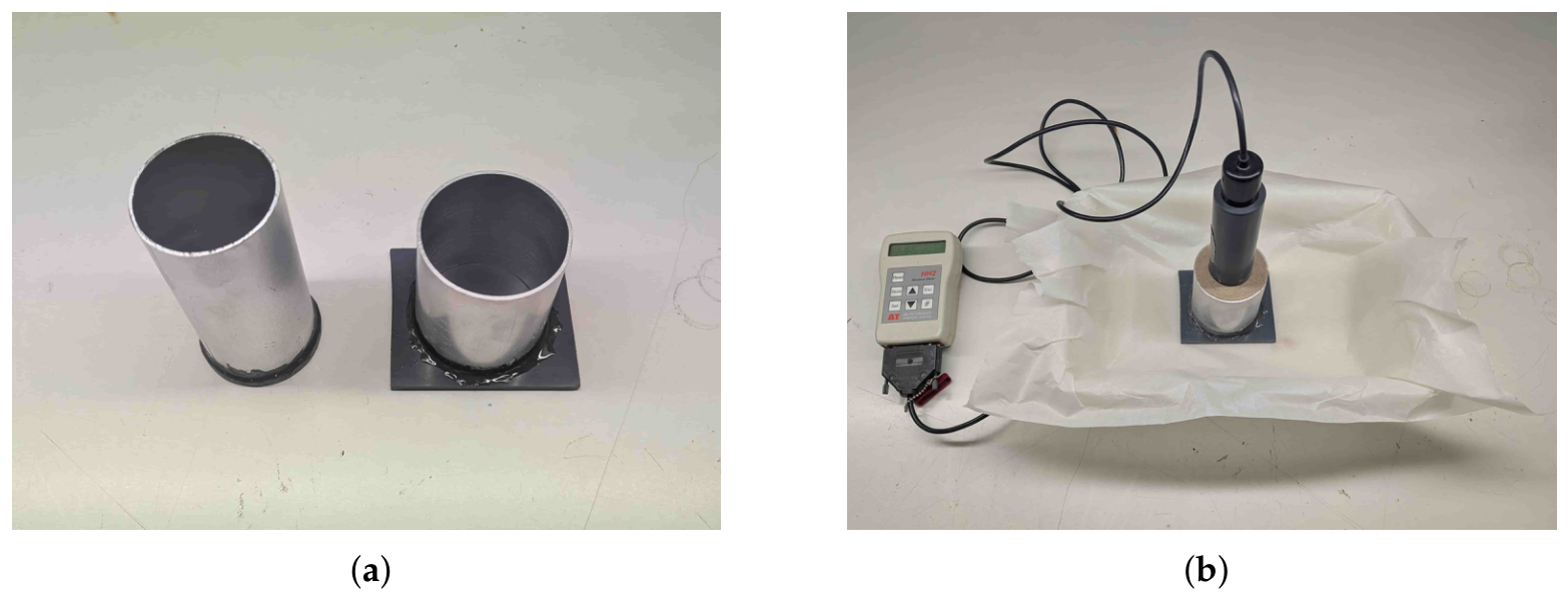
Successive moisture levels were prepared by the following unpack–wet–repack cycle. The soil was removed from the container and spread on a tray, and a controlled mass of distilled water was added to raise the VMC by 5%. For the container volume, each 5% increment corresponds to
added as distilled water (density 1 g/cm3). The wetted soil was thoroughly mixed and left sealed for one hour to allow capillary redistribution, then repacked into the container following the same lift-and-tamp procedure to preserve the packing state, and the probe voltage was recorded for that moisture level. Repeating this cycle produced calibration points at and . The visual appearance of the soil at each moisture level is shown in Figure A2.
Figure A2.
Visual aspect of the soil sample in the tray at each prepared volumetric moisture level during the ThetaProbe calibration, from oven-dry (%) to saturation-approaching (%). Each level was obtained by adding 13.7 g of distilled water (Equation (A16)) to the previous state, mixing, and equilibrating for one hour before the probe reading.
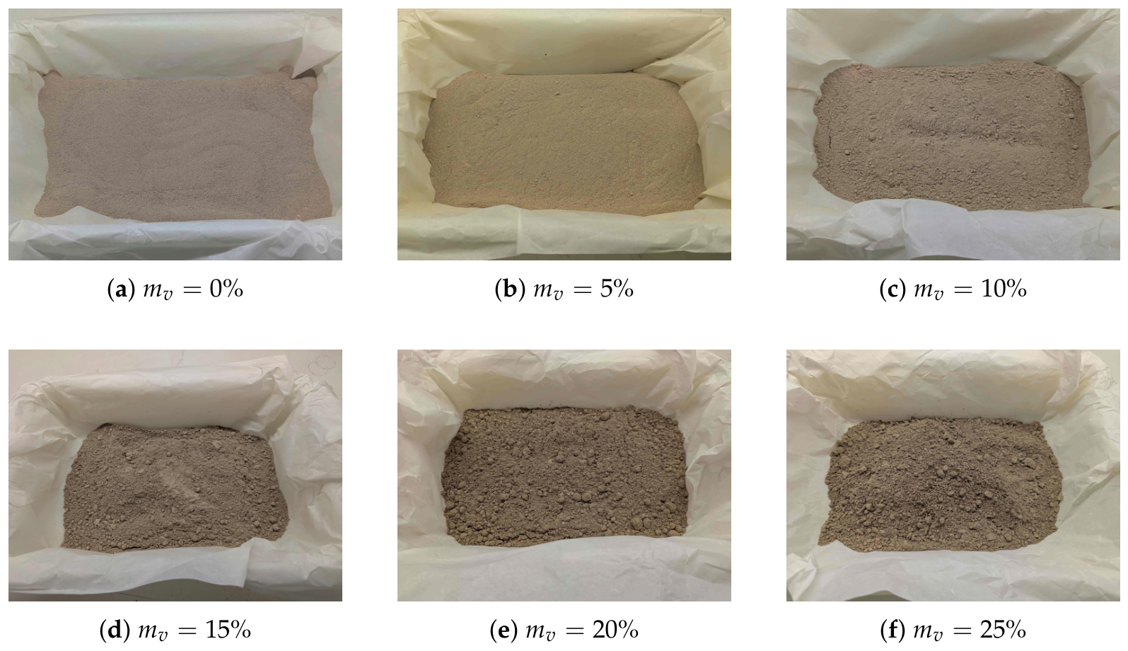
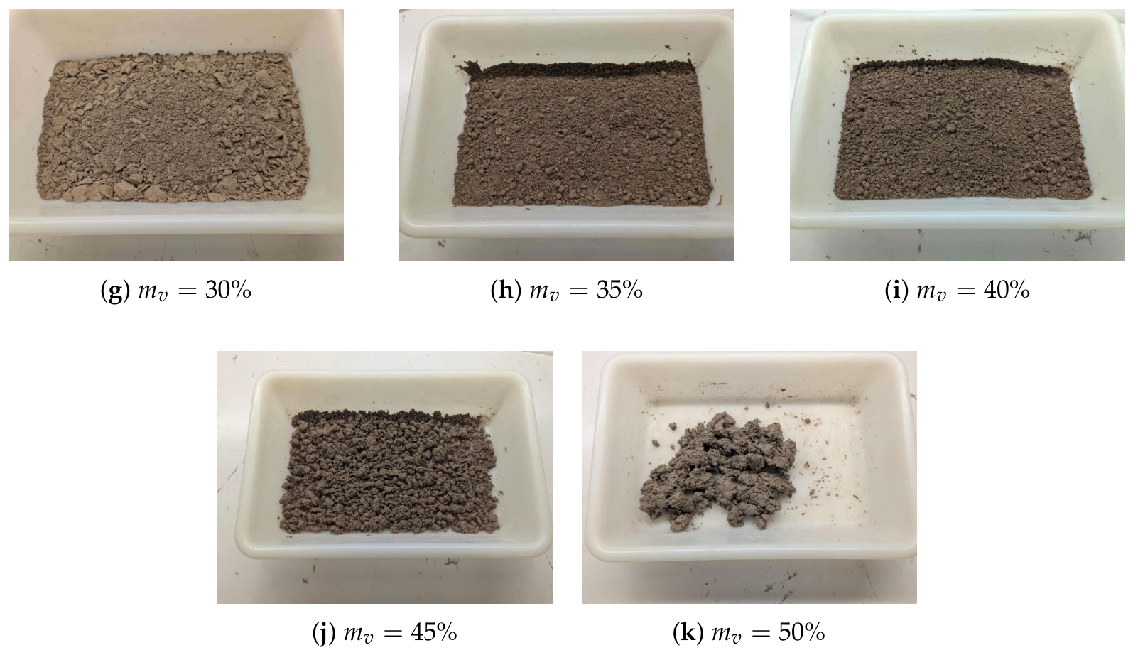
Appendix B.2. Coefficient Retrieval
At each moisture level, the recorded probe voltage (V) was converted to through the manufacturer’s third-order polynomial of Equation (16), and the pairs were fitted by linear regression to obtain the offset and slope of Equation (17). Figure A3 shows the calibration points and the fitted lines.
Three fitting ranges are compared: the full measured range () and two restricted ranges, and . The full-range fit departs from linearity at the highest moisture level, where the soil approaches saturation and the – relationship is known to flatten; excluding the point alone reduces the residual scatter from to VMC. Removing the point in addition brings only a marginal further improvement ( VMC), which does not justify the loss of support at the wet end: the two wettest layers prepared in Phase B retrieve at and , so a calibration truncated at would have to be extrapolated beyond its own fitting range to convert them. The fit was therefore adopted, as the widest range that both excludes the saturation knee and contains every moisture state measured in this work. Table A1 summarizes the comparison, and the adopted fit yields
with an essentially linear response over the workable moisture range spanned by the experiment. The corresponding residual statistics are VMC, VMC, and a maximum absolute residual of VMC. These coefficients were subsequently applied, via the inversion of Equation (17), to the probe voltages recorded during Phases B and C, providing accurate volumetric moisture readings for each prepared layer.
Table A1.
Comparison of the three candidate fitting ranges for the ThetaProbe soil-specific calibration. The residual metrics are expressed in VMC units (i.e., divided by the fitted slope ), which is the quantity that propagates to the retrieved moisture. The range in bold is the one adopted in this work.
Figure A3.
ThetaProbe soil-specific calibration: square root of the relative permittivity, , obtained from the probe output voltage via Equation (16), against VMC (). The linear fits over the full range (, red), the adopted workable range (, green), and the narrower range (blue) are shown; the adopted fit yields the calibration coefficients of Equation (A17).
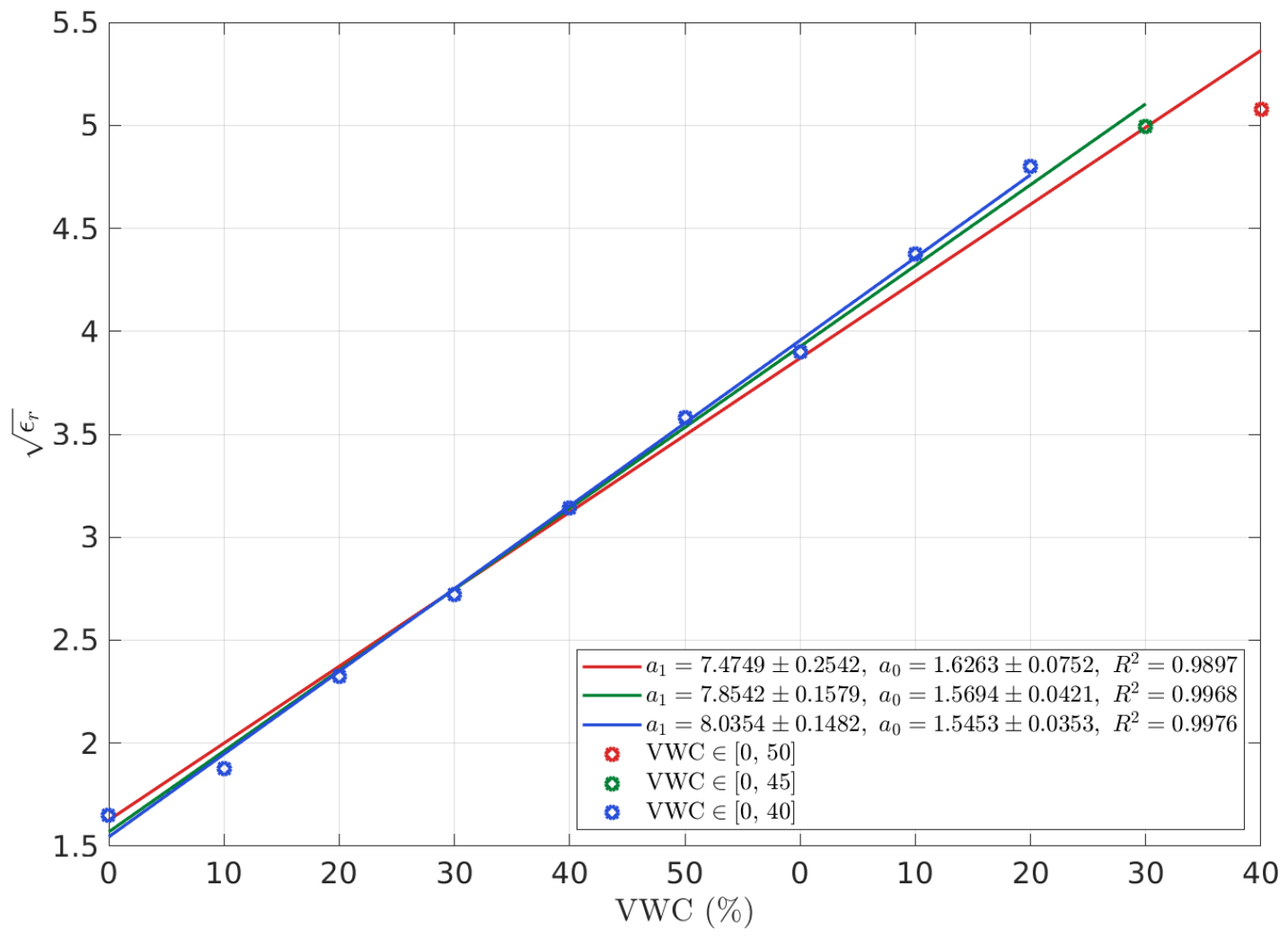
Appendix C. Soil Texture Characterization: Hydrometer Method
This appendix details the determination of the soil particle-size distribution by the Bouyoucos hydrometer method [26], whose sedimentation principle and the VMC-independent textural fractions it yields are summarized in Section 3.2. The procedure separates the sample into sand, silt, and clay mass fractions from two hydrometer readings taken at standardized settling times, each corrected against a soil-free blank prepared with the same dispersing solution. The analysis was performed on three independent soil samples, and the reported texture is the mean of the three.
Appendix C.1. Materials Needed
- 100 soil sample,
- 1 sieve,
- 2× graduated cylinders,
- 1× Bouyoucos hydrometer,
- 1× Thermometer,
- 1× Scale with 0.1 g precision,
- 2× beakers,
- 1× Magnetic stirrer,
- 2 of distilled water,
- 50 of sodium hexametaphosphate (dispersing agent),
- pH test strips.
Appendix C.2. Procedure
Appendix C.2.1. Step 1—Sample Preparation
The soil sample was oven-dried at 105 °C for to remove all soil moisture (%), then passed through a sieve to remove coarse fragments. Using an oven-dry mass is essential so that represents the true dry mass of mineral solids against which the settled fractions are normalized.
Appendix C.2.2. Step 2—Dispersing Solution
A dispersing solution was prepared by dissolving of sodium hexametaphosphate in of distilled water, stirred on a magnetic stirrer for several hours to ensure complete dissolution. The dispersant deflocculates clay aggregates so that particles settle individually rather than as clumps. The solution pH was verified to lie between 7 and 9, adjusting with sodium carbonate if required.
Appendix C.2.3. Step 3—Soil-Dispersant Mixture
In total, of the oven-dried and sieved soil sample ( g) was combined with of distilled water and of the dispersing solution, and left to stand overnight to allow full aggregate breakdown before sedimentation.
Appendix C.2.4. Step 4—Sedimentation Readings
The mixture was stirred vigorously with the magnetic stirrer for , then transferred to a graduated sedimentation cylinder (rinsing with distilled water to ensure complete particle transfer) and topped up with distilled water to the 1000 mL mark. The cylinder was shaken back and forth for , placed on the bench, and the timer started ().
Two settling times were used for the analysis. At each, the hydrometer reading (R) was taken at the base of the meniscus and the suspension temperature (T) recorded:
- 40 s reading (): The hydrometer was inserted at and read at . By this time all sand-sized particles have settled below the hydrometer bulb, so the reading reflects the mass of silt and clay still in suspension.
- 2 h reading (): only clay-sized particles remain in suspension, so the reading reflects the clay mass alone.
Three replicate readings were taken at each settling time. At the suspension was re-shaken before each of the three readings, since the rapid settling of coarse particles makes the reading time-sensitive and a fresh, fully-mixed start is required for repeatability. At the three readings were taken consecutively without re-shaking, as the slow clay settling makes the reading effectively stationary over the short interval between replicates.
A soil-free blank, containing only distilled water and dispersing solution in the same proportions, was measured simultaneously at each settling time (, ) and at the same temperature as the soil suspension.
Appendix C.2.5. Step 5—Calculations
Each soil reading was corrected by subtracting its simultaneous blank,
which removes the contribution of the dispersing solution to the suspension density. Because the blank is read at the same temperature as the sample, no separate temperature correction is required. The combined silt-and-clay and the clay mass fractions follow directly from the corrected readings, normalized by the oven-dry sample mass:
The sand and silt fractions are then obtained by difference:
Appendix C.3. Readings and Results
The procedure was carried out for three independent soil samples to improve precision. Hydrometer readings for each of the three replicate samples and their simultaneous blanks are collected in Table A2. Note that the soil readings are already the three measurements averaged. Applying Equations (A18)–(A22) to each sample and averaging yields the mean textural composition given in Table A3.
Table A2.
Bouyoucos hydrometer readings (R, in ) for the three soil replicates and the soil-free blank, at the two settling times used in the analysis. Each entry is the mean of three replicate readings.
Table A3.
Textural fractions derived for each replicate and their mean. The mean composition classifies the soil as a silt loam.
With a mean composition of % sand, % silt, and % clay, the soil is classified as a silt loam according to the USDA textural triangle. These sand and clay fractions provide the S and C inputs to the dielectric models of Section 2.2.
Appendix C.4. Procedure Photographs
Figure A4.
Stages of the Bouyoucos hydrometer analysis, from sample preparation through the two sedimentation readings. (a) The 100 g soil sample oven-drying. (b) The 50 g soil sample 2 mm sieved. (c) Dispersing solution (25 sodium hexametaphosphate + 500 distilled water). (d) Dispersing solution pH check. (e) Soil-dispersant mixture (50 soil + 100 dispersing solution + 250 distilled water). (f) Soil-dispersant mixture after lying overnight. (g) Soil-dispersant mixture transferred to graduated cylinder, filled with distilled water until 1000 mL. (h) First reading at 40 s. (i) Second reading at 2 h.
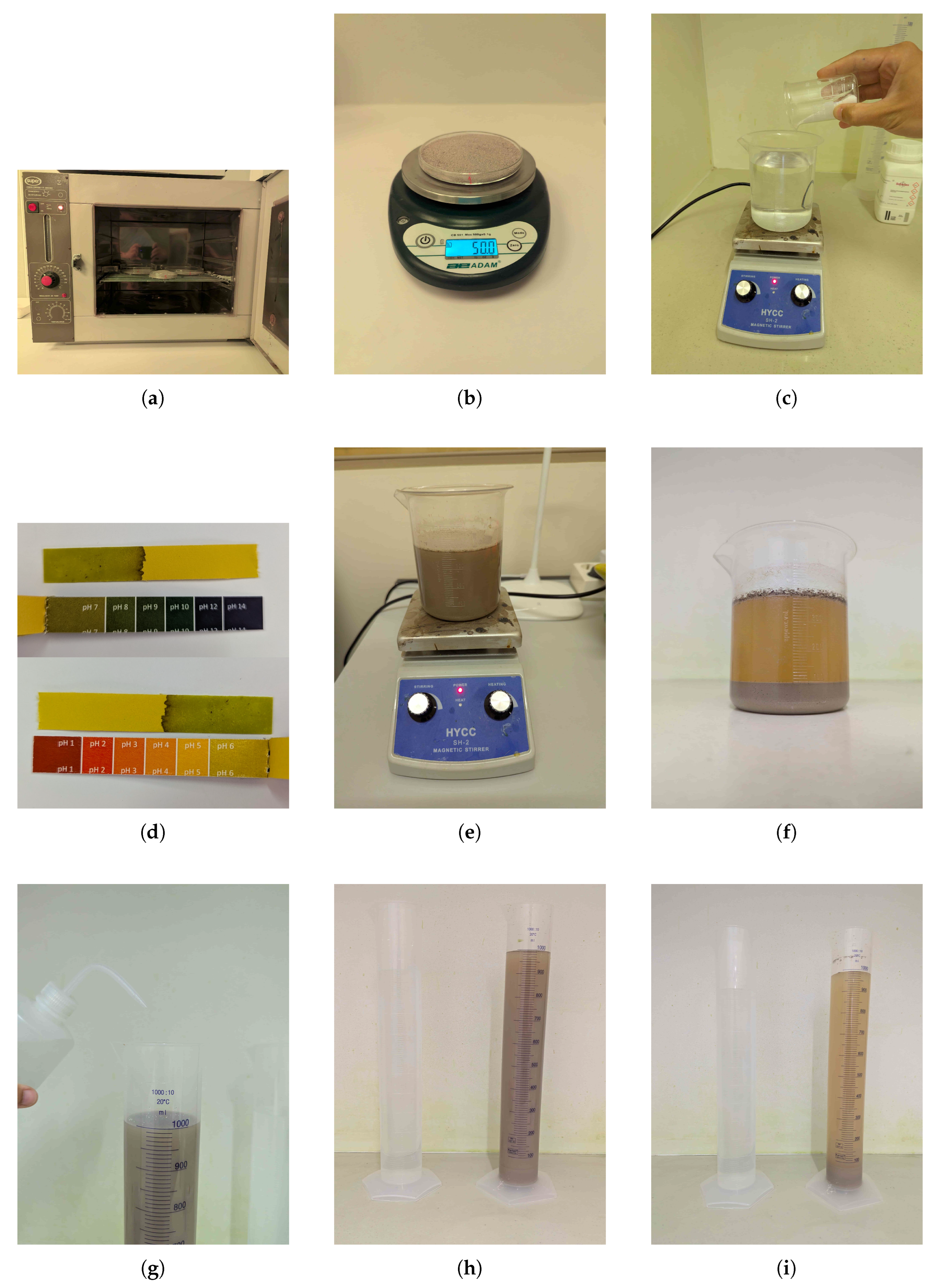
Appendix D. Additional Material from Phase B and Phase C Experimental Campaigns
Figure A5.
Tray films of thickness made of PET (, ) are included explicitly in the model. Their effect is bounded: over – GHz and across every soil state measured here (gray traces), the 4 films change by at most dB, of which at most dB is dielectric absorption within the film itself, the remainder being impedance mismatch and electrical thickness. In the differential observable used for the analysis the films are common to the wet and the baseline measurement and largely cancel, leaving a residual of at most dB.
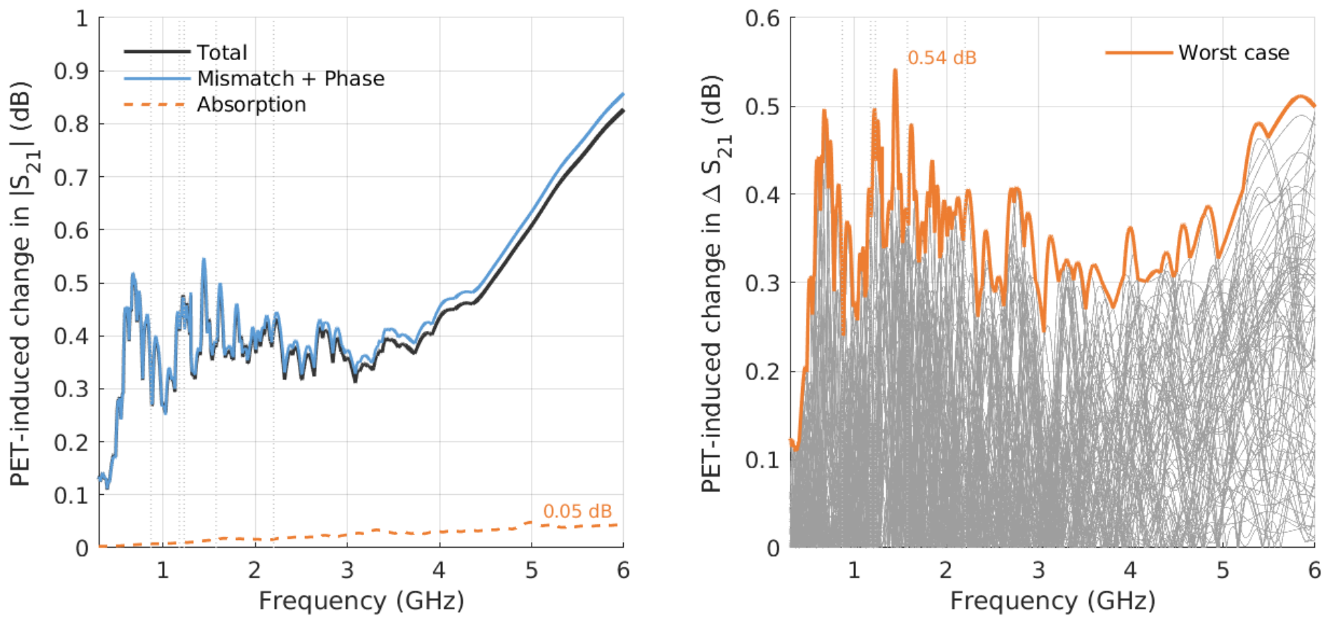
Figure A6.
Phase B and with the wet tray in L2, for the different VMC levels. Center and right plots are normalized with respect to the Phase A baseline, including simulation results from both soil dielectric models.
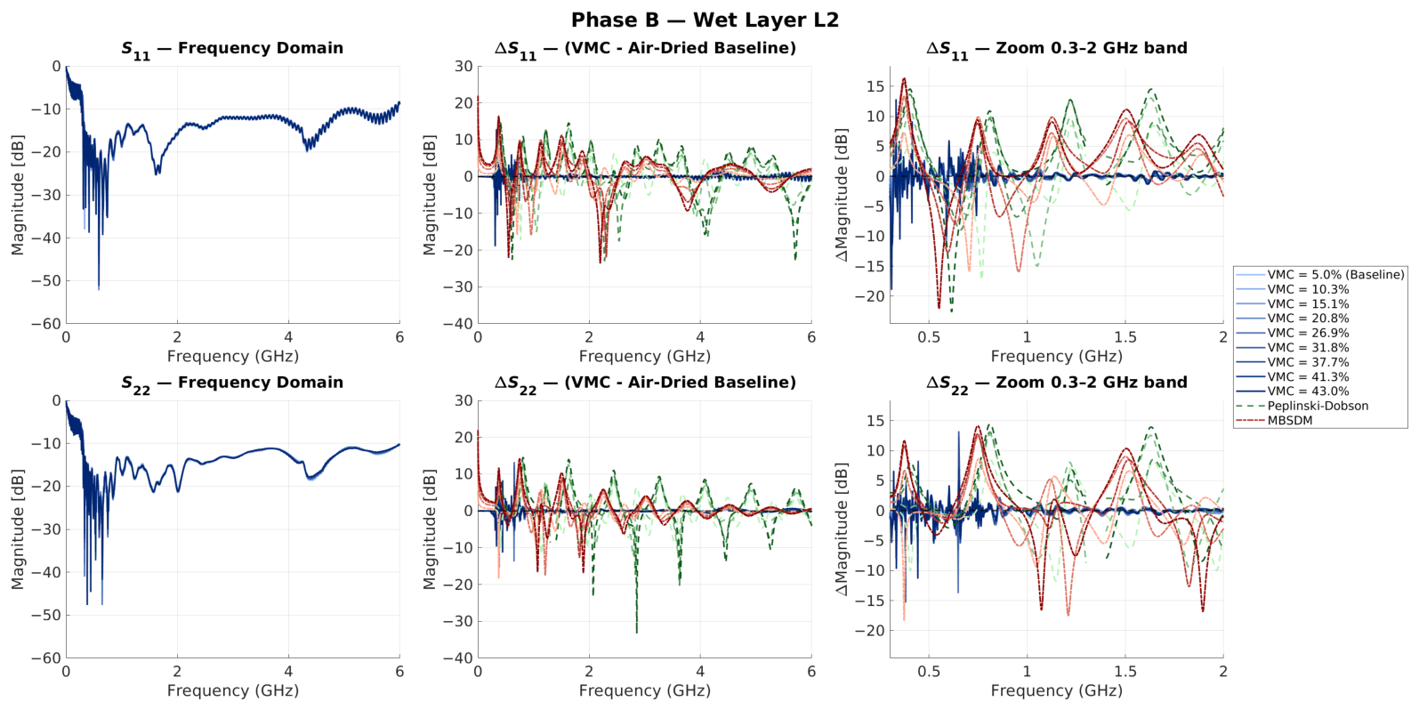
Figure A7.
As Figure A6, with the wet tray in L3.
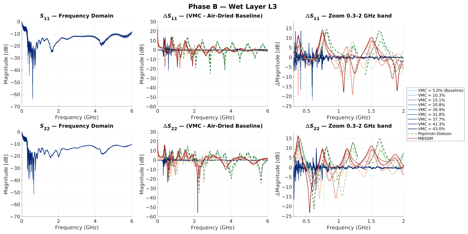
Figure A8.
As Figure A6, with the wet tray in L4.
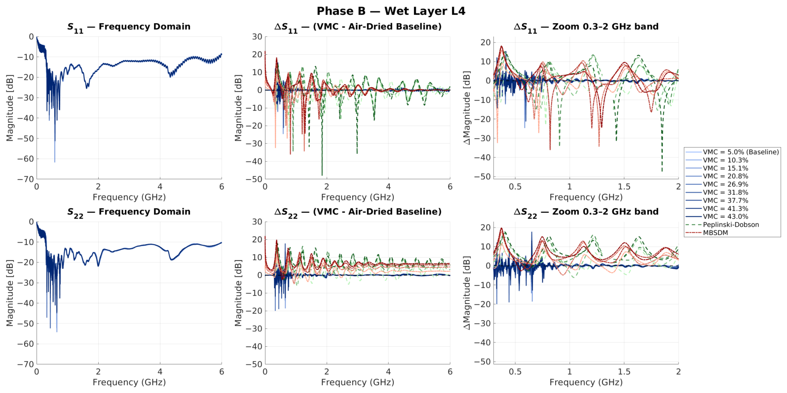
Figure A9.
Phase B with the wet tray in L2, for the different VMC levels. Center and right plots are normalized with respect to the baseline measurement taken during Phase A, including the simulation results from both soil dielectric models.
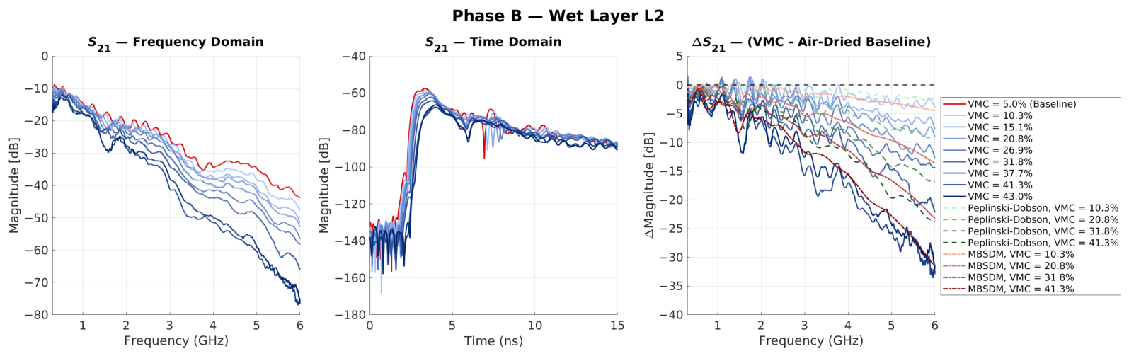
Figure A10.
As Figure A9, with the wet tray in L3.
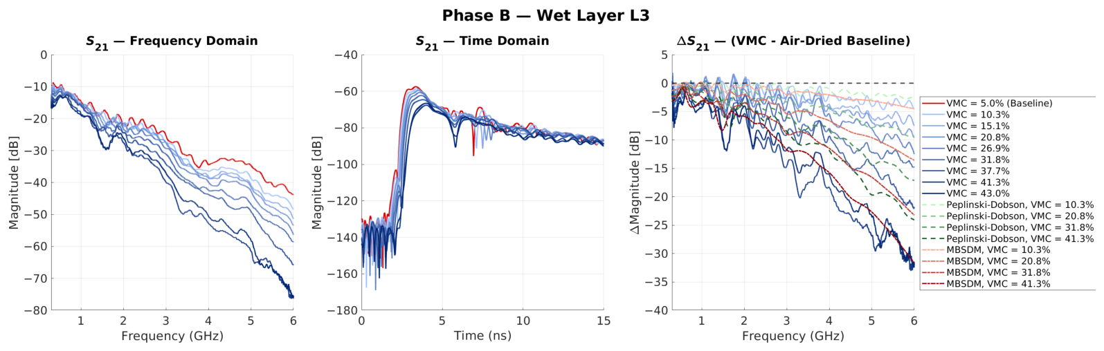
Figure A11.
As Figure A9, with the wet tray in L4.
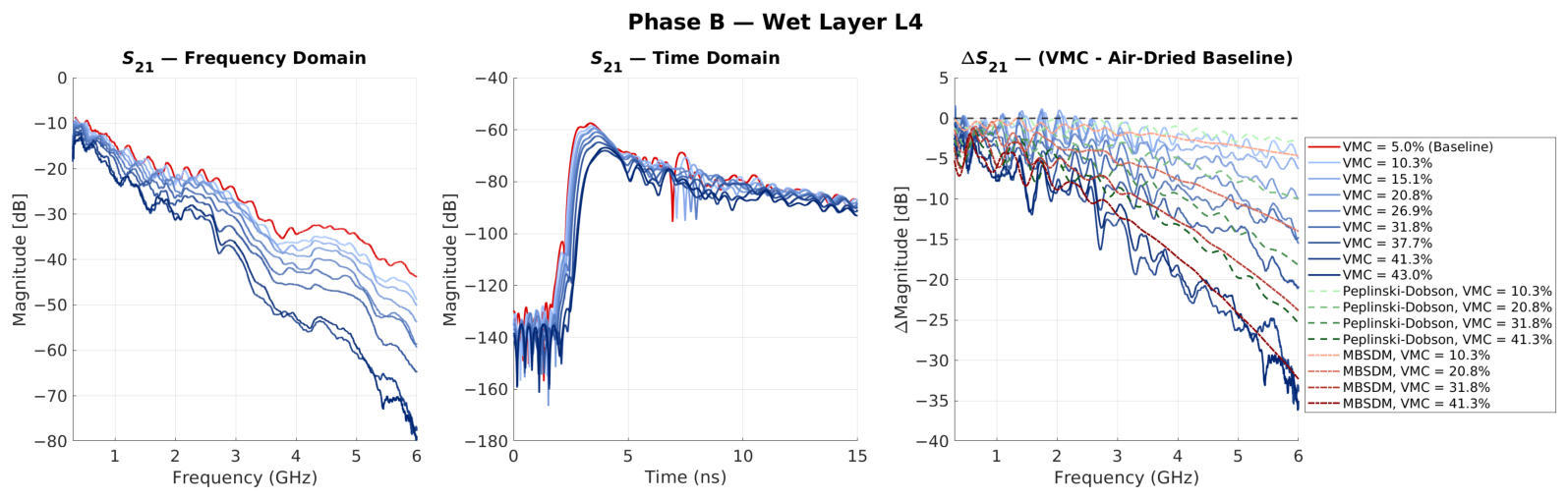
Figure A12.
Phase C measured for the different numbers of wet layers. Each plot overlaps the different combinations of wet layer positions together with results from simulations with Peplinski–Dobson and MBSDM soil dielectric modeling.
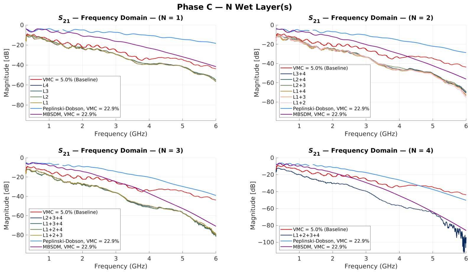
Figure A13.
Trend of measurements with Savitzky–Golay de-rippling order 3, 0.90 GHz window, and modeled transmissivity values used for the best-fit comparison between the two dielectric models.
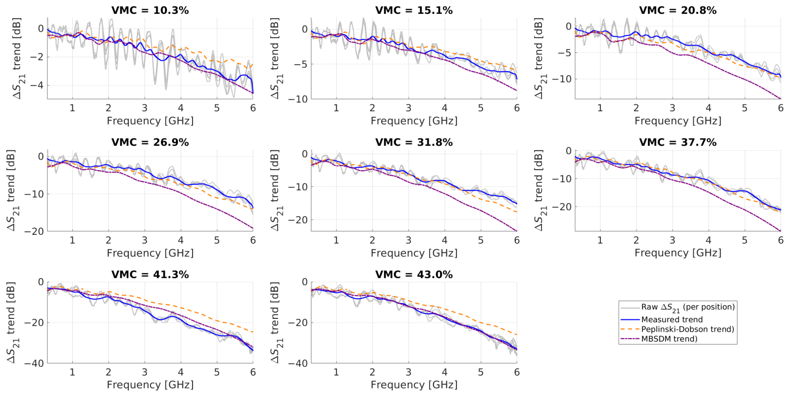
Figure A14.
Sensitivity of the dielectric-model selection to the Savitzky–Golay de-rippling, over the same grid as Table 4: rows are the eight moisture levels, columns the six 1 GHz scoring bins. The selector was re-run at 21 filter settings (orders 2–4; spans – the GHz fringe period, i.e., – GHz). Letters give the model selected at the operating point used throughout (order 3, GHz): P for Peplinski–Dobson, M for the MBSDM. Green marks cells won by the same model at every setting, amber those whose winner changes with the filter; blank cells were not scored.
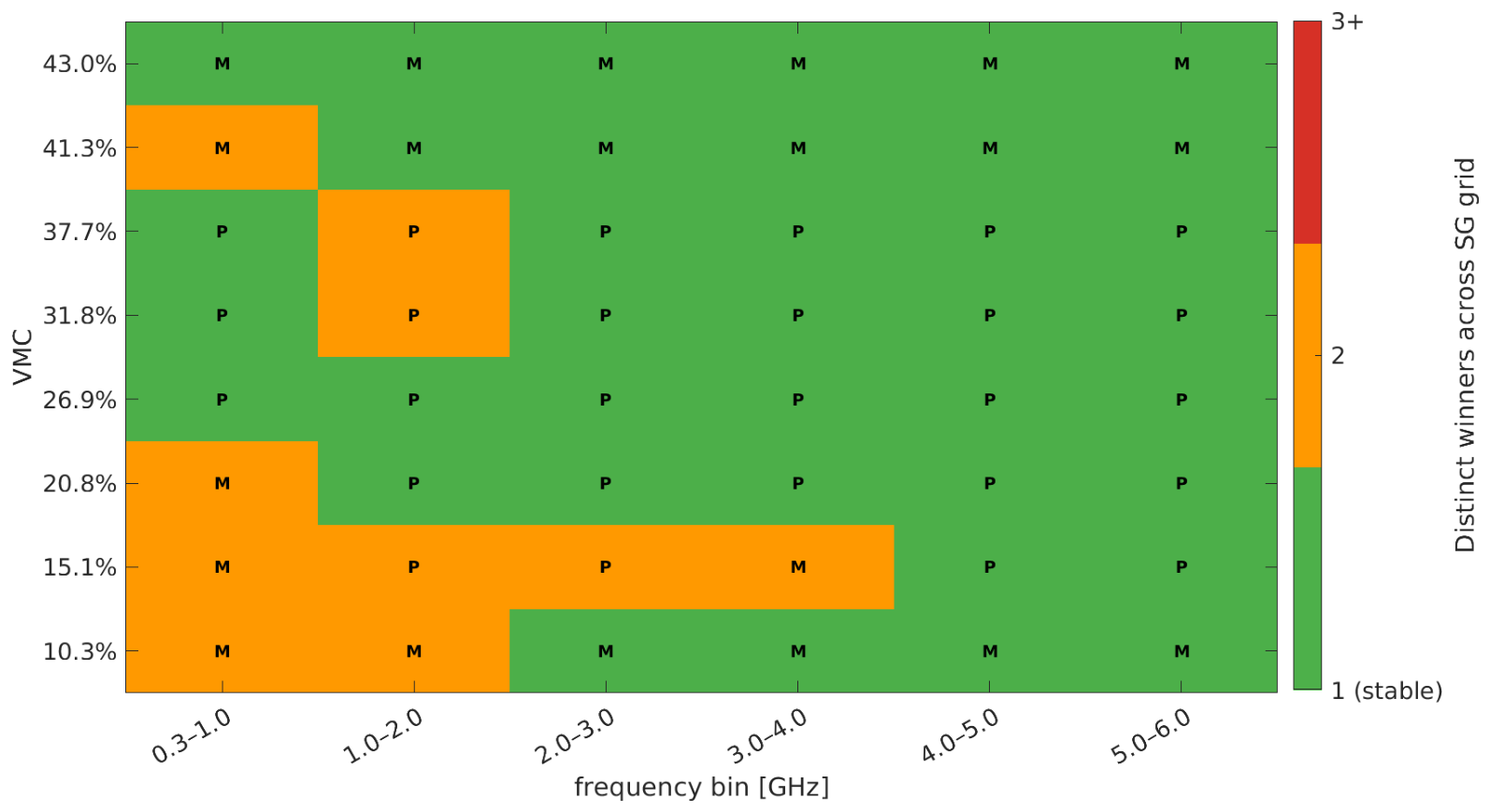
Appendix E. Robustness of the Model Selection to Forward-Model Error
The model selection of Section 5.4 scores each candidate dielectric model by the RMSE between the measured and simulated , which presumes that the forward model of Section 4 is structurally correct. It is not exactly so: as stated in Section 3.1, the column is interrogated in the antenna near field while the transfer matrix assumes normal-incidence plane-wave propagation over the geometric column thickness, and finite-aperture illumination, antenna–soil coupling and the cavity response are represented only through the differencing against the air-dry baseline. The measured–simulated residual therefore contains both dielectric-model error and forward-model structural error, and a lower RMSE need not identify the model that better describes the soil permittivity. This appendix tries to bound that possibility without having a material of known permittivity.
Synthetic Recovery of a Known Dielectric Model
One dielectric model is treated as ground truth and its generated with the forward model of Section 4 for all 32 configurations of the position sweep. That trace is then corrupted with the terms of Equation (35) that do not cancel in the differential observable: a residual level offset and gain slope standing for the uncanceled part of and of the unmeasured , the coherent cavity term at the GHz fringe period with random phase, trace noise at the session-to-session repeatability of the air-dry baseline, and a multiplicative scale on the effective propagation path. No dielectric error is injected at any point, so the permittivity of each run is exact and every misselection observed downstream is attributable to forward-model error alone. The corrupted trace is scored by the identical pipeline used for Table 4: the same Savitzky–Golay de-rippling at order 3 over a GHz span, the same 1 GHz bins, the Peplinski–Dobson validity gap excluded from both candidates, and the winner taken as the lower RMSE. The experiment is then repeated with the other model as truth, over 200 draws per configuration.
The selector returns the true model in of the 76,800 cell-draws. The failures are confined to the –1 GHz bin at the driest states, where recovery falls to 79, 88 and at , and respectively and is at or above everywhere else in the map. This is the expected behavior rather than a defect: those are the cells in which the two models predict almost the same attenuation, and their RMSE margins in Table 4 are correspondingly , and dB. Conditioning the recovery rate on the margin makes the correspondence explicit: above an observed margin of dB every margin bin recovers the true model in at least of draws, and the cells falling below that threshold are exactly the three named above.
This test does not validate the forward model against a material of known permittivity. The synthetic test establishes that the selector recovers a known dielectric model under an assumed error budget, so its conclusion is conditional on that budget being representative; the amplitudes were fixed from the measured residuals and the ripple period from the stack geometry, but they are not themselves measured quantities.
References
- Kerr, Y.H.; Waldteufel, P.; Wigneron, J.P.; Delwart, S.; Cabot, F.; Boutin, J.; Escorihuela, M.J.; Font, J.; Reul, N.; Gruhier, C.; et al. The SMOS Mission: New Tool for Monitoring Key Elements of the Global Water Cycle. Proc. IEEE 2010, 98, 666–687. [Google Scholar] [CrossRef] [Scilit]
- Entekhabi, D.; Njoku, E.G.; O’Neill, P.E.; Kellogg, K.H.; Crow, W.T.; Edelstein, W.N.; Entin, J.K.; Goodman, S.D.; Jackson, T.J.; Johnson, J.; et al. The Soil Moisture Active Passive (SMAP) Mission. Proc. IEEE 2010, 98, 704–716. [Google Scholar] [CrossRef] [Scilit]
- Njoku, E.G.; Entekhabi, D. Passive microwave remote sensing of soil moisture. J. Hydrol. 1996, 184, 101–129. [Google Scholar] [CrossRef] [Scilit]
- Zavorotny, V.; Voronovich, A. Scattering of GPS signals from the ocean with wind remote sensing application. IEEE Trans. Geosci. Remote Sens. 2000, 38, 951–964. [Google Scholar] [CrossRef] [Scilit]
- Zavorotny, V.U.; Gleason, S.; Cardellach, E.; Camps, A. Tutorial on Remote Sensing Using GNSS Bistatic Radar of Opportunity. IEEE Geosci. Remote Sens. Mag. 2014, 2, 8–45. [Google Scholar] [CrossRef] [Scilit]
- Rodriguez-Alvarez, N.; Bosch-Lluis, X.; Camps, A.; Vall-llossera, M.; Valencia, E.; Marchan-Hernandez, J.; Ramos-Perez, I. Soil Moisture Retrieval Using GNSS-R Techniques: Experimental Results Over a Bare Soil Field. IEEE Trans. Geosci. Remote Sens. 2009, 47, 3616–3624. [Google Scholar] [CrossRef] [Scilit]
- Camps, A.; Park, H.; Pablos, M.; Foti, G.; Gommenginger, C.P.; Liu, P.W.; Judge, J. Sensitivity of GNSS-R Spaceborne Observations to Soil Moisture and Vegetation. IEEE J. Sel. Top. Appl. Earth Obs. Remote Sens. 2016, 9, 4730–4742. [Google Scholar] [CrossRef] [Scilit]
- Munoz-Martin, J.F.; Llaveria, D.; Herbert, C.; Pablos, M.; Park, H.; Camps, A. Soil Moisture Estimation Synergy Using GNSS-R and L-Band Microwave Radiometry Data from FSSCat/FMPL-2. Remote Sens. 2021, 13, 994. [Google Scholar] [CrossRef] [Scilit]
- Camps, A.; Park, H.; Castellví, J.; Corbera, J.; Ascaso, E. Single-Pass Soil Moisture Retrievals Using GNSS-R: Lessons Learned. Remote Sens. 2020, 12, 2064. [Google Scholar] [CrossRef] [Scilit]
- Rodriguez-Alvarez, N.; Bosch-Lluis, X.; Camps, A.; Ramos-Perez, I.; Valencia, E.; Park, H.; Vall-llossera, M. Vegetation Water Content Estimation Using GNSS Measurements. IEEE Geosci. Remote Sens. Lett. 2012, 9, 282–286. [Google Scholar] [CrossRef] [Scilit]
- Humphrey, V.; Frankenberg, C. Continuous ground monitoring of vegetation optical depth and water content with GPS signals. Biogeosciences 2023, 20, 1789–1811. [Google Scholar] [CrossRef] [Scilit]
- Ulaby, F.T. Microwave Radar and Radiometric Remote Sensing; The University of Michigan Press: Ann Arbor, MI, USA, 2014. [Google Scholar]
- Escorihuela, M.; Chanzy, A.; Wigneron, J.; Kerr, Y. Effective soil moisture sampling depth of L-band radiometry: A case study. Remote Sens. Environ. 2010, 114, 995–1001. [Google Scholar] [CrossRef] [Scilit]
- Njoku, E.G.; Kong, J.A. Theory for passive microwave remote sensing of near-surface soil moisture. J. Geophys. Res. 1977, 82, 3108–3118. [Google Scholar] [CrossRef] [Scilit]
- Farr, T.; Elachi, C.; Hartl, P.; Chowdhury, K. Microwave Penetration and Attenuation in Desert Soil: A Field Experiment with the Shuttle Imaging Radar. IEEE Trans. Geosci. Remote Sens. 1986, GE-24, 590–594. [Google Scholar] [CrossRef] [Scilit]
- Owe, M.; Van de Griend, A.A. Comparison of soil moisture penetration depths for several bare soils at two microwave frequencies and implications for remote sensing. Water Resour. Res. 1998, 34, 2319–2327. [Google Scholar] [CrossRef] [Scilit]
- Dobson, M.; Ulaby, F.; Hallikainen, M.; El-rayes, M. Microwave Dielectric Behavior of Wet Soil-Part II: Dielectric Mixing Models. IEEE Trans. Geosci. Remote Sens. 1985, GE-23, 35–46. [Google Scholar] [CrossRef] [Scilit]
- Peplinski, N.; Ulaby, F.; Dobson, M. Dielectric properties of soils in the 0.3-1.3-GHz range. IEEE Trans. Geosci. Remote Sens. 1995, 33, 803–807. [Google Scholar] [CrossRef] [Scilit]
- Mironov, V.; Kosolapova, L.; Fomin, S. Physically and Mineralogically Based Spectroscopic Dielectric Model for Moist Soils. IEEE Trans. Geosci. Remote Sens. 2009, 47, 2059–2070. [Google Scholar] [CrossRef] [Scilit]
- O’Neill, P.; Bindlish, R.; Chan, S.; Chaubell, J.; Njoku, E.; Jackson, T. Algorithm Theoretical Basis Document (ATBD) for the SMAP Level 2 & 3 Soil Moisture (Passive) Data Products, Revision F; JPL D-66480; Jet Propulsion Laboratory, California Institute of Technology: La Cañada Flintridge, CA, USA, 2020. Available online: https://smap.jpl.nasa.gov/system/internal_resources/details/original/484_L2_SM_P_ATBD_rev_F_final_Aug2020.pdf (accessed on 25 June 2026).
- European Space Agency. Algorithm Theoretical Basis Document (ATBD) for the SMOS Level 2 Soil Moisture Processor Development Continuation Project, Ref SO-TN-ARR-L2PP-0037. Issue 4.0. 2019. Available online: https://earth.esa.int/eogateway/documents/20142/37627/SMOS-L2-SM-ATBD.pdf (accessed on 28 October 2025).
- Kong, J.A. Electromagnetic Wave Theory; EMW Publishing: Cambridge, MA, USA, 2000. [Google Scholar]
- Hallikainen, M.; Ulaby, F.; Dobson, M.; El-rayes, M.; Wu, L.k. Microwave Dielectric Behavior of Wet Soil-Part 1: Empirical Models and Experimental Observations. IEEE Trans. Geosci. Remote Sens. 1985, GE-23, 25–34. [Google Scholar] [CrossRef] [Scilit]
- Mironov, V.L.; Bobrov, P.P.; Fomin, S.V. Multirelaxation Generalized Refractive Mixing Dielectric Model of Moist Soils. IEEE Geosci. Remote Sens. Lett. 2013, 10, 603–606. [Google Scholar] [CrossRef] [Scilit]
- Lambot, S.; Andre, F. Full-Wave Modeling of Near-Field Radar Data for Planar Layered Media Reconstruction. IEEE Trans. Geosci. Remote Sens. 2014, 52, 2295–2303. [Google Scholar] [CrossRef] [Scilit]
- Bouyoucos, G.J. Hydrometer Method Improved for Making Particle Size Analyses of Soils. Agron. J. 1962, 54, 464–465. [Google Scholar] [CrossRef] [Scilit]
- Gee, G.W.; Bauder, J.W. Particle-size Analysis. In Methods of Soil Analysis: Part 1 Physical and Mineralogical Methods, 5.1, 2nd ed.; American Society of Agronomy: Madison, WI, USA, 1986. [Google Scholar] [CrossRef] [Scilit]
- Institut Cartogràfic i Geològic de Catalunya. Mapa geològic de Catalunya Geotreball IV. Mapa de sòls Ivars d’Urgell 360-2-2 (66-28). 2014. Available online: https://app1.icgc.cat/bd/mapes/icgc_GT4_360q22_66x28_v1g.pdf (accessed on 30 July 2026).
- Delta-T Devices. ThetaProbe ML2x User Manual; Delta-T Devices Ltd.: Cambridge, UK, 1998; Available online: https://delta-t.co.uk/wp-content/uploads/2016/11/ML2-Thetaprobe-UM.pdf (accessed on 8 July 2026).
- Delta-T Devices. Moisture Meter HH2 User Manual; Delta-T Devices Ltd.: Cambridge, UK, 2017; Available online: https://delta-t.co.uk/wp-content/uploads/2016/10/HH2-UM-4.2.pdf (accessed on 8 July 2026).
- Matula, S.; Báťková, K.; Legese, W. Laboratory Performance of Five Selected Soil Moisture Sensors Applying Factory and Own Calibration Equations for Two Soil Media of Different Bulk Density and Salinity Levels. Sensors 2016, 16, 1912. [Google Scholar] [CrossRef] [Scilit] [PubMed]
- Rohde & Schwarz. VNA ZNB3020. Available online: https://www.rohde-schwarz.com/es/productos/test-y-medida/analizadores-de-redes-vectoriales/rs-znb3000-vector-network-analyzer_334291.html (accessed on 17 July 2026).
- Harris, F. On the use of windows for harmonic analysis with the discrete Fourier transform. Proc. IEEE 1978, 66, 51–83. [Google Scholar] [CrossRef] [Scilit]
- Rohde & Schwarz. ZV-Z1XX Calibration Kits. Available online: https://www.rohde-schwarz.com/us/products/test-and-measurement/vna-accessories/rs-zn-z1xx-network-analyzer-calibration-kits-economy_63493-747623.html (accessed on 17 July 2026).
- Mini-Circuits. CBL-1.5M-SMSM+. Available online: https://www.minicircuits.com/WebStore/dashboard.html?model=CBL-1.5M-SMSM%2B (accessed on 17 July 2026).
- Lambot, S.; Slob, E.; van den Bosch, I.; Stockbroeckx, B.; Vanclooster, M. Modeling of ground-penetrating Radar for accurate characterization of subsurface electric properties. IEEE Trans. Geosci. Remote Sens. 2004, 42, 2555–2568. [Google Scholar] [CrossRef] [Scilit]
- Born, M.; Wolf, E.; Bhatia, A.B.; Clemmow, P.C.; Gabor, D.; Stokes, A.R.; Taylor, A.; Wayman, P.A.; Wilcock, W.L. Principles of Optics; Cambridge University Press: Cambridge, UK, 1999; p. 952. [Google Scholar]
- Singh, K.P.; Ranjan, R.; Deshpande, R. Design of a wideband Balun for Archimedean spiral antenna in energy harvesting. In Proceedings of the 2015 International Conference on Applied and Theoretical Computing and Communication Technology (iCATccT); IEEE: New York, NY, USA, 2015; pp. 45–49. [Google Scholar] [CrossRef] [Scilit]
- Savitzky, A.; Golay, M.J.E. Smoothing and Differentiation of Data by Simplified Least Squares Procedures. Anal. Chem. 1964, 36, 1627–1639. [Google Scholar] [CrossRef] [Scilit]
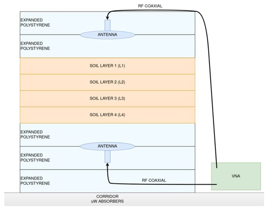
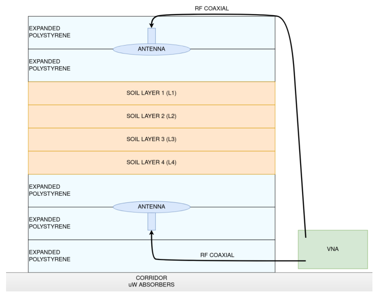
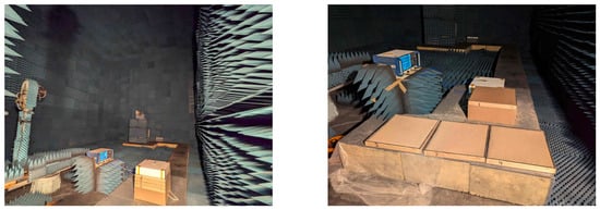
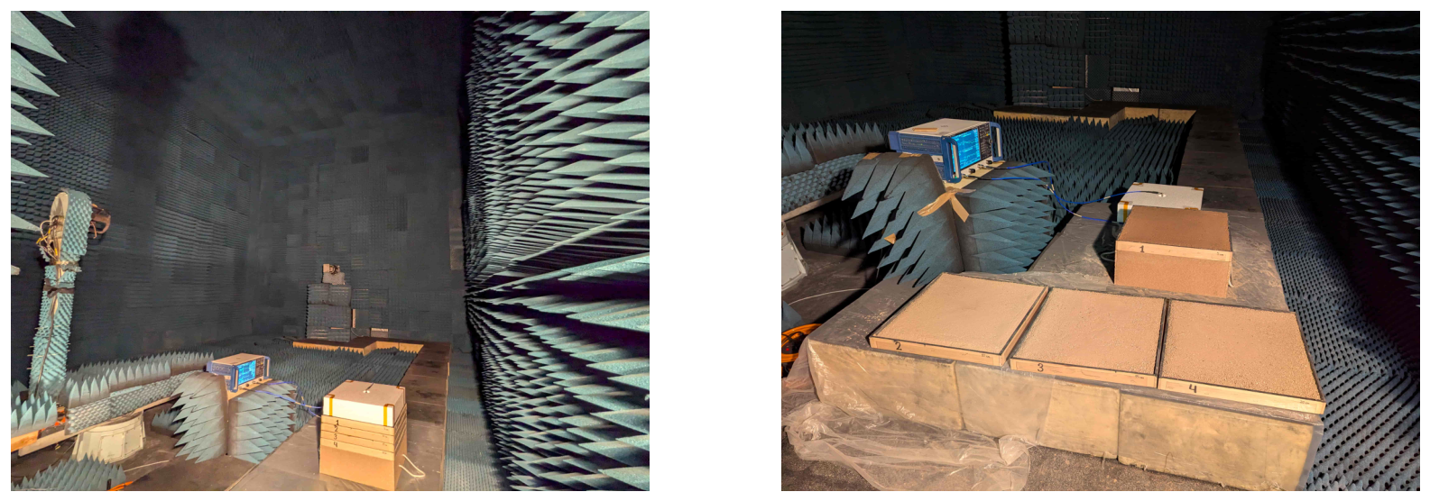
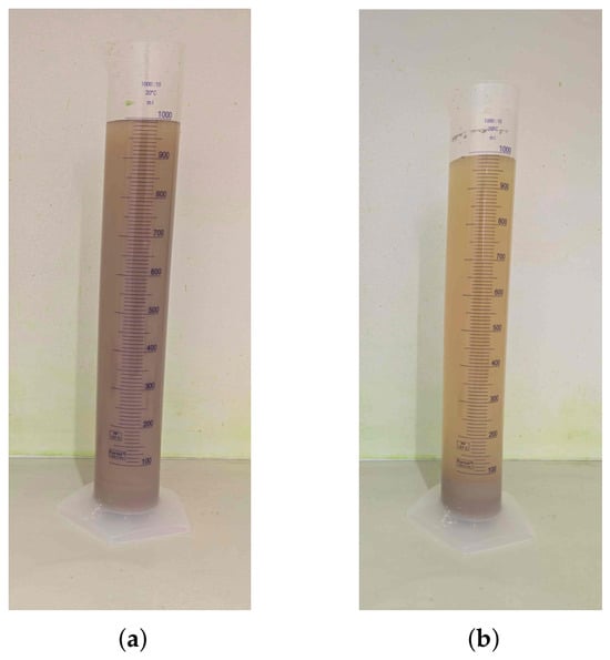
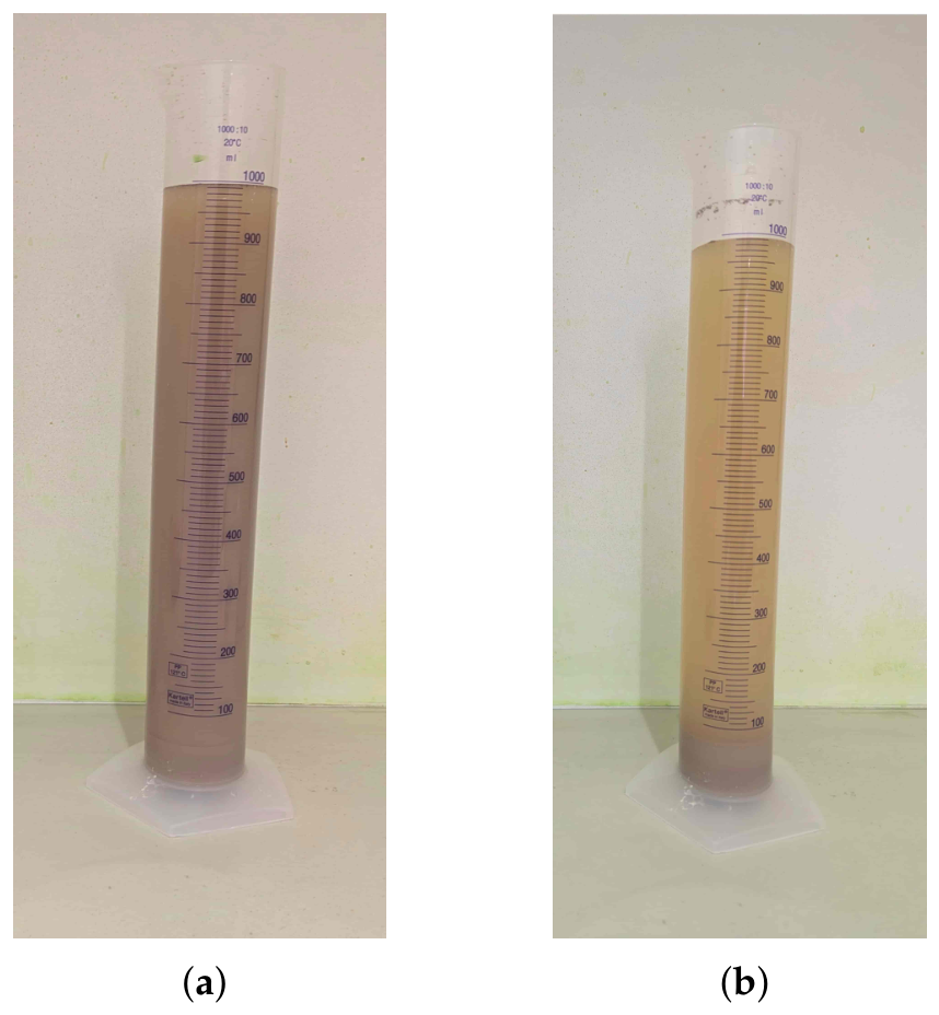
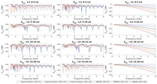
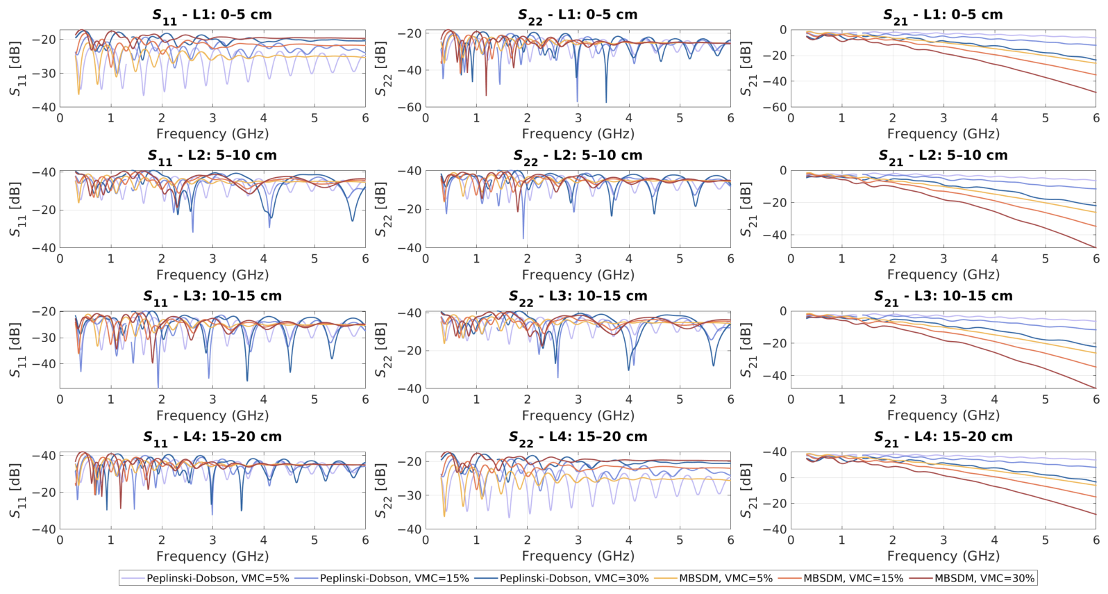
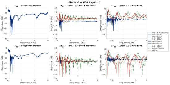
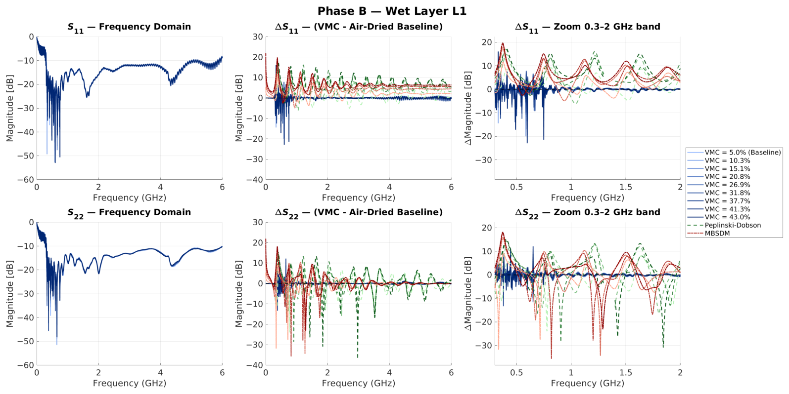
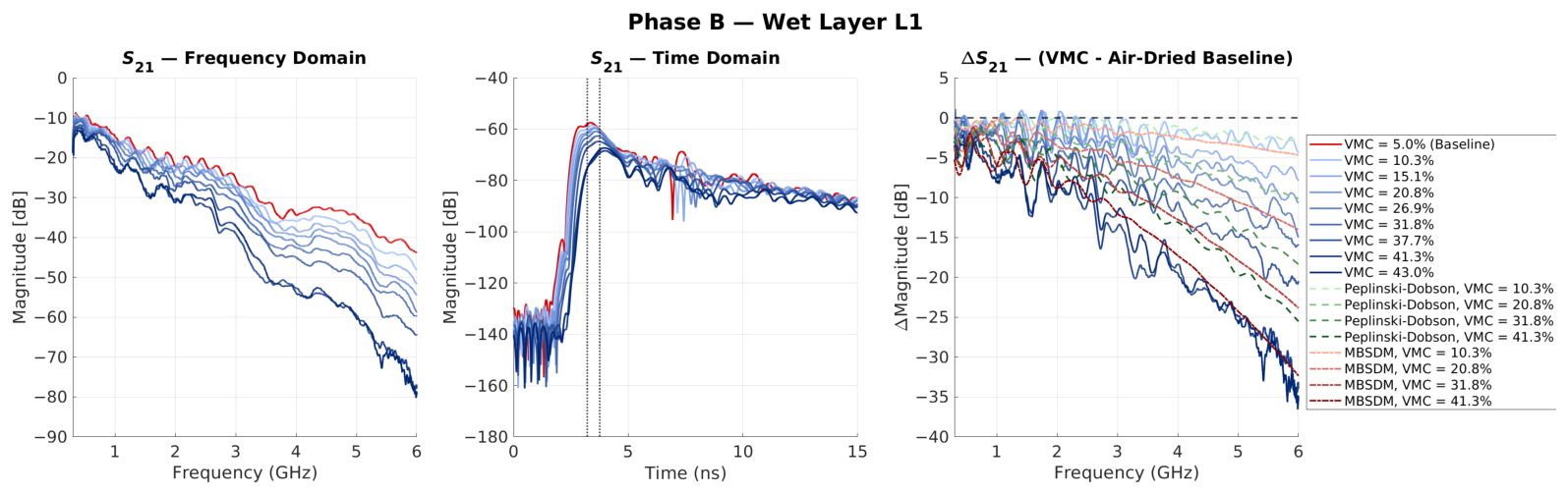
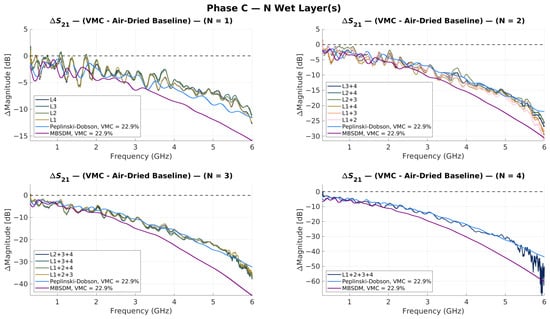
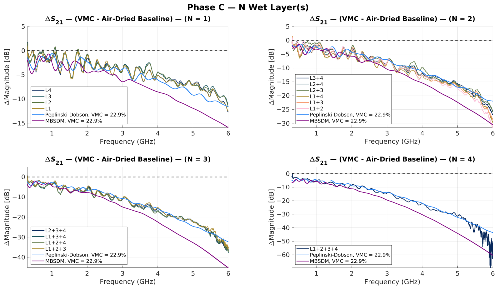
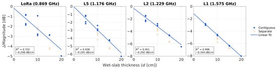
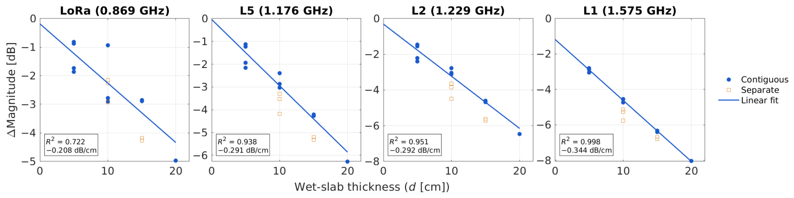
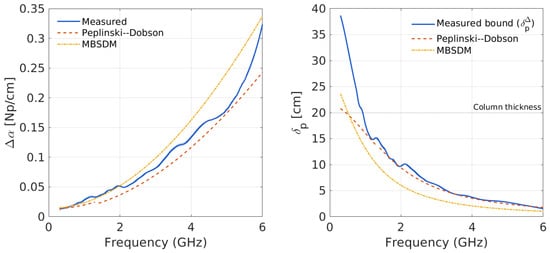
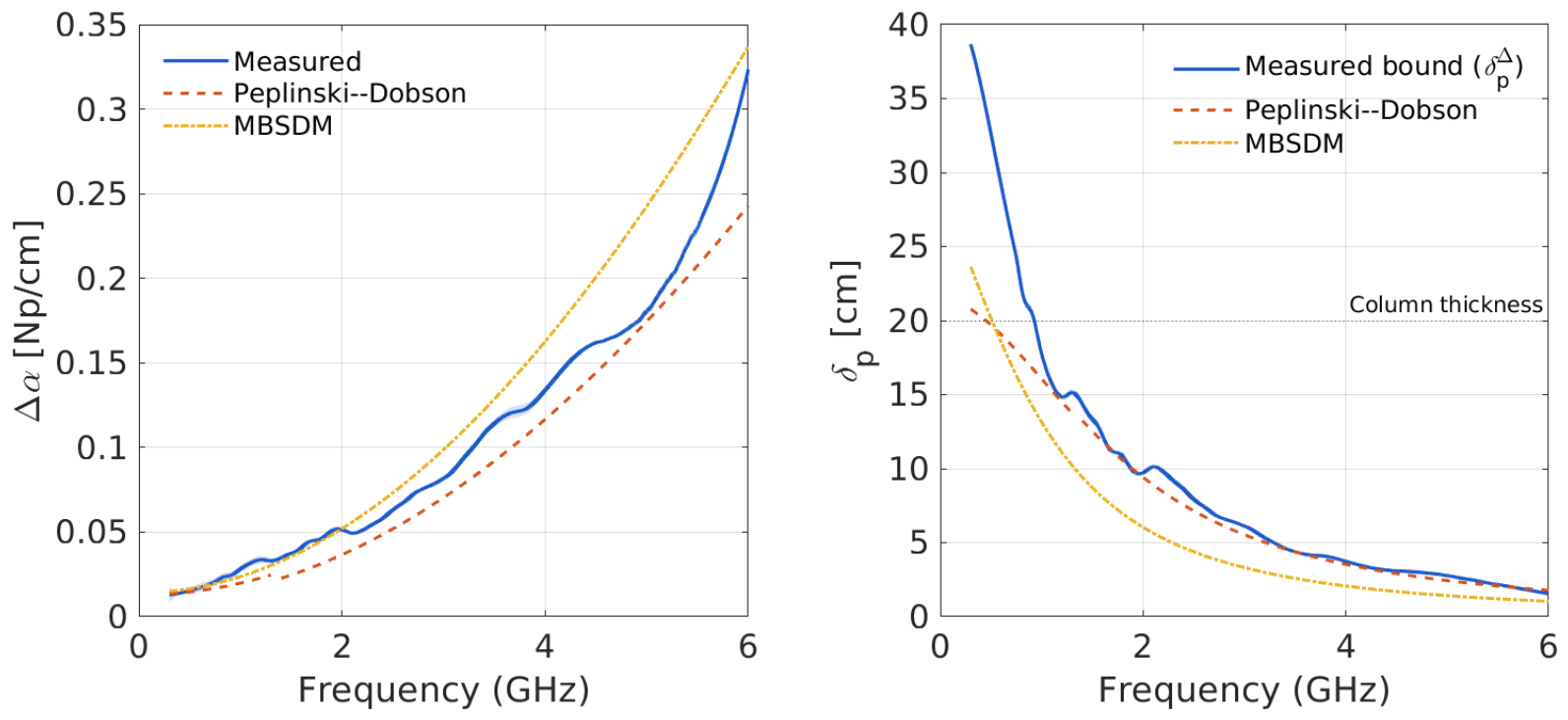

Disclaimer/Publisher’s Note: The statements, opinions and data contained in all publications are solely those of the individual author(s) and contributor(s) and not of MDPI and/or the editor(s). MDPI and/or the editor(s) disclaim responsibility for any injury to people or property resulting from any ideas, methods, instructions or products referred to in the content. |
© 2026 by the authors. Licensee MDPI, Basel, Switzerland. This article is an open access article distributed under the terms and conditions of the Creative Commons Attribution (CC BY) license.