Abstract
In this paper, hyperspectral imaging technology, combined with chemometrics methods, was used to detect the nitrogen content of soybean leaves, and to achieve the rapid, non-destructive and in situ detection of the nitrogen content in soybean leaves. Soybean leaves under different fertilization treatments were used as the research object, and the hyperspectral imaging data and the corresponding nitrogen content data of soybean leaves at different growth stages were obtained. Seven spectral preprocessing methods, such as Savitzky–Golay smoothing (SG), first derivative (1-Der), and direct orthogonal signal correction (DOSC), were used to establish the quantitative prediction models for soybean leaf nitrogen content, and the quantitative prediction models of different spectral preprocessing methods for soybean leaf nitrogen content were analyzed and compared. On this basis, successive projections algorithm (SPA), genetic algorithm (GA) and random frog (RF) were employed to select the characteristic wavelengths and compress the spectral data. The results showed the following: (1) The full-spectrum prediction model of soybean leaf nitrogen content based on DOSC pretreatment was the best. (2) The PLS model of soybean leaf nitrogen content based on the five characteristic wavelengths had the best prediction performance. (3) The spatial distribution map of soybean leaf nitrogen content was generated in a pixel manner using the extracted five characteristic wavelengths and the DOSC-RF-PLS model. The nitrogen content level of soybean leaves can be quantified in a simple way; this provides a foundation for rapid in situ non-destructive detection and the spatial distribution difference detection of soybean leaf nitrogen. (4) The overall results illustrated that hyperspectral imaging technology was a powerful tool for the spatial prediction of the nitrogen content in soybean leaves, which provided a new method for the spatial distribution of the soybean nutrient status and the dynamic monitoring of the growth status.
1. Introduction
Soybean (Glycine max (L.) Merrill) is an important source of plant protein and vegetable oi for human beings. It has a wide range of uses worldwide, such as for food, vegetable oil, and feed [1]. There is a huge gap between China’s soybean supply and consumption demand. Therefore, it is an important measure to solve the contradiction between the supply and demand of soybean in China and ensure the safety of the soybean industry and national grain and oil security by improving the yield and quality of soybean in China and increasing the proportion of soybean cultivation [2].
Nitrogen is an important part of protein, nucleic acid, phospholipid, chlorophyll and some hormones in soybean plants, and it is also one of the important factors limiting soybean growth and high yield. The rapid and effective monitoring of the nitrogen content during soybean growth is an important prerequisite and foundation for guiding soybean fertilization and achieving high quality and high yield of soybean. Chemical methods, such as Kjeldahl nitrogen determination, indophenol blue colorimetric, and Dumas combustion, are commonly used for nitrogen detection. These methods have problems of long detection cycle, complex operation, and destructiveness, which make the continuous determination of nitrogen in time and space impossible [3].
Hyperspectral imaging technology is an organic combination of spatial imaging technology and spectral technology. The image information and spectral information of the research object could be obtained at the same time using hyperspectral imaging technology. So, it is an effective tool to study the internal information content and spatial distribution of the research object [4,5]. The hyperspectral imaging technology has been successfully applied in remote sensing, food, agriculture, microbiology and pharmaceutical fields [6,7]. In addition, the detection of crop nitrogen content based on hyperspectral imaging technology has achieved good results in wheat, corn, rapeseed, citrus and other crops. Hyperspectral imaging technology was applied to measure the nitrogen content in wheat leaves, and the regional spatial distribution map of the nitrogen content in wheat leaves at flagging and flowering stages was generated [8]. Goel et al. analyzed the hyperspectral images of maize canopy under nitrogen stress and weed stress, and found that the spectral reflectance at 498 nm and 671 nm could effectively reflect the difference in nitrogen levels in maize [9]. By using the spectrum–graph unity feature of hyperspectral imaging technology, differences in nitrogen content within the same leaf or among different leaves can be analyzed intuitively and effectively [10,11]. However, to the best of our knowledge, few studies have been conducted to study the distribution of the nitrogen content in soybean leaves based on hyperspectral imaging technology; the relationship between the spectral reflectance of soybean leaves and the leaf nitrogen content is not clear, and it remains to be demonstrated whether the use of hyperspectral imaging technology can realize the effective detection and continuous monitoring of the nitrogen content of soybean leaves.
Therefore, in this study, the relationship between the spectra of soybean leaves and nitrogen content under different fertilization treatments was analyzed, the effects of spectral pre-processing and characteristic wavelength selection methods on the prediction model of the nitrogen content of soybean leaves were investigated, and the optimal detection model for the detection of the nitrogen content of soybean leaves was optimized. On this basis, the spatial distribution map of soybean leaf nitrogen content was generated to provide a new method for the spatial prediction of the soybean nutrient status and the dynamic monitoring of the growth status, which, in turn, provided a basis for the application of fertilizer decisions during soybean growth.
2. Materials and Methods
2.1. Experimental Materials
The experiment was conducted from March to August 2017 in the experimental base of the National Engineering Research Centre of Intelligent Equipment for Agriculture, Xiaotangshan Town, Changping District, Beijing, China (116°44′ E, 40°18′ N). This area has a warm-temperate continental semi-humid and semi-arid monsoon climate, with an average annual temperature of 11.8 °C, an average annual frost-free period of 203 days, an average annual sunshine hour of 2816 h, and an average annual precipitation of 584 mm. In order to eliminate the influence of uncontrollable factors, such as rainfall, high temperature, disease, etc., the soybean varieties of Zhonghuang 13 and Qihuang 35 were planted in a greenhouse. Three-factor quadratic orthogonal regression was used to quantitatively fertilize the soybean to obtain the nitrogen gradient in order to obtain soybean leaf samples with a certain concentration of the nitrogen gradient. Urea was applied as nitrogen fertilizer in the experiment, and the range of nitrogen application was 0~70 kg/hm2. The specific fertilization scheme is shown in Table 1. Each soybean variety was set up with 15 fertilizer treatments and one control treatment (no fertilization). There was a total of 32 treatments for the two varieties, and 4 replicates were set up under each treatment. The fully expanded soybean leaves at the top were collected as experimental samples during the soybean seedling stage (14 May 2017), flowering stage (7 June 2017), podding stage (28 June 2017) and seed-filling stage (20 July 2017). The collected soybean leaves were subjected to hyperspectral imaging data collection and leaf-nitrogen-content detection. Two samples were collected under each treatment in each sampling period, and a total of 256 samples were collected in 4 sampling periods.

Table 1.
Design table of quadratic orthogonal regression experiment for soybean fertilization.
2.2. Hyperspectral Imaging Data Acquisition
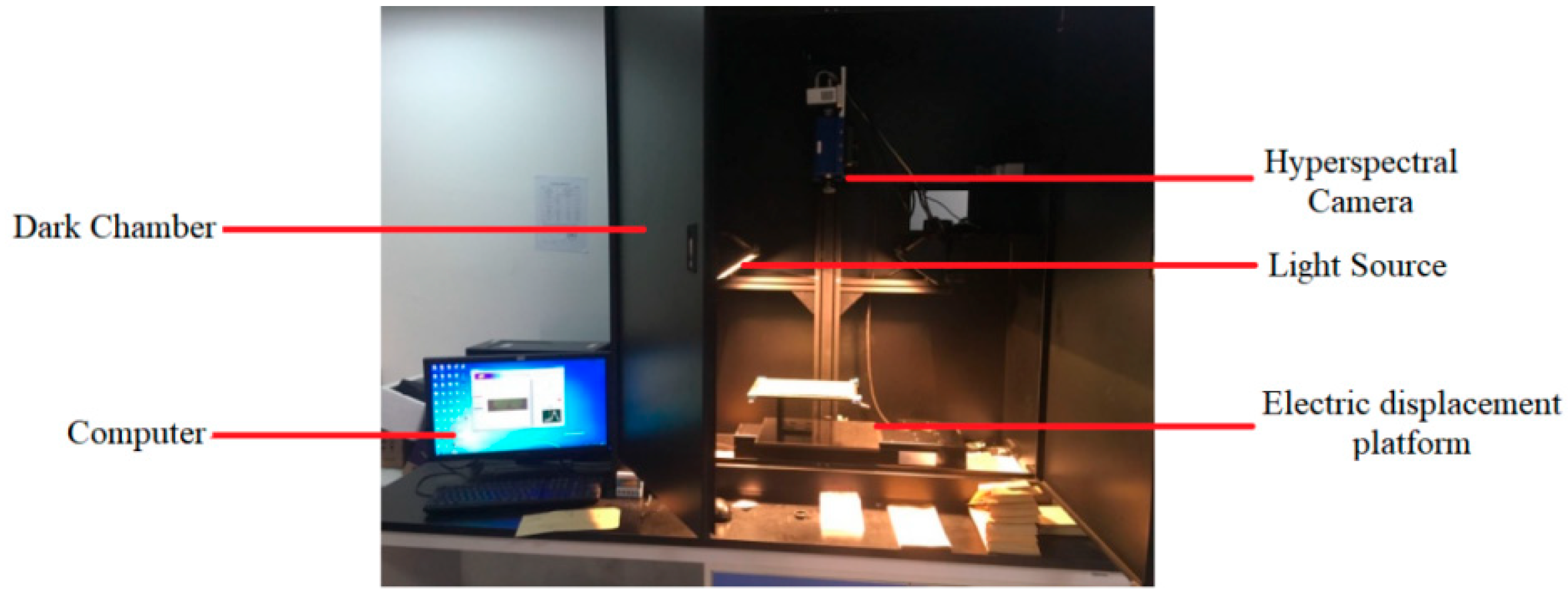
The visible near-infrared hyperspectral imaging system (ImSpector V10E, SPECIM company, Oulu, Finland) was used to collect the hyperspectral imaging data of soybean leaves. The system is composed of a light source, hyperspectral camera, CCD detector, imaging lens, closed light box, electronically controlled displacement platform and computer (as shown in Figure 1). The light sources used in the study were two 150 W halogen lamps (2900-ER, Illumination, New York, NY, USA), which can provide continuous and smooth light information between 380~2000 nm bands. The hyperspectral camera has a spectral scanning range of 400~1000 nm, a spectral resolution of 2.8 nm, a spectral interval of 0.65 nm, and a pixel size of 1344 (rows) × 1024 (columns). During the experiment, the distance between the object and the camera was 60 cm, and the actual size of the object represented by one pixel in the image was 0.16 nm.
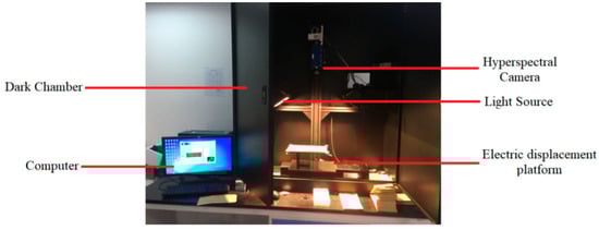
Figure 1.
Hyperspectral imaging system on leaf scale.
Before collecting hyperspectral imaging data, the system was preheated for 30 min to ensure its stability. The moving speed of the electronically controlled displacement platform was set to be 1.15 mm/s, the exposure time was 10 ms, and the vertical distance between the hyperspectral camera and the sample was 80 cm. In order to reduce the influence of instrument sensitivity and light source change on hyperspectral imaging data, the standard whiteboard (a rectangular white board composed of polytetrafluoroethylene material) and dark current need to be corrected during each measurement. The calibration process was carried out according to Formula (1) as follows:
In the formula, Iraw was the original hyperspectral imaging data of soybean leaves, Iwhite was whiteboard data captured with the light turned on, Idark was current data obtained through covering the lens without illumination, and R (raw spectra) was the corrected hyperspectral imaging data of soybean leaves.
2.3. Determination and Data Division of Nitrogen Content in Soybean Leaves
After the hyperspectral imaging data of soybean leaves were collected, the leaf samples were immediately placed in an oven at 105 °C for 30 min, and then dried to constant weight at 80 °C. The dried samples were crushed and passed through the stainless steel mesh. After screening, 0.25 g of the sample was weighed and boiled with concentrated sulfuric acid, and then the nitrogen content of soybean leaves was determined by AA3 continuous flow analyzer combined with a standard curve.
The abnormal values of soybean nutrient chemical value data were eliminated by 3 times the standard deviation. At the same time, the abnormal spectral samples of the extracted leaf spectral curves were eliminated by the Monte Carlo algorithm. A total of 11 abnormal samples were eliminated, and 245 soybean samples including leaf nitrogen content and hyperspectral imaging data were finally obtained. The Kennard–Stone (K-S) classification algorithm was used to divide the soybean leaf samples into a calibration set and a prediction set according to the ratio of 3:1 (as shown in Table 2). There were 184 samples in the calibration set, and the range of the nitrogen content in the calibration set was between 8.275~44.724 mg/g. Due to the fact that the modeling set sample contains a large range and has a good representativeness, it is beneficial to establish a stable soybean leaf-nitrogen-content prediction model.
Table 2.
Statistics of N value of soybean leaves in the calibration and prediction sets.
2.4. Spectral Preprocessing
When the data were obtained by the hyperspectral image acquisition system, the noise signals (such as high frequency random noise, baseline drift, sample heterogeneity, etc.) were often collected synchronously. In order to improve the stability and prediction accuracy of the nitrogen content model of soybean leaves, it is necessary to preprocess the raw spectra [12]. Spectral data were pretreated to remove spectral noise and other disturbances using Savitzky–Golay smoothing (SG), multiple scattering correction (MSC), standard normal variate (SNV), de-trending processing, first differential (1-Der), second differential (2-Der), and direct orthogonal signal correction (DOSC). Thereby, the correlation between spectral reflectance and the nitrogen content of soybean leaves was enhanced. A relatively good spectral preprocessing method was determined by evaluating the performance of the partial least squares regression (PLSR) model.
2.5. Selection Method of Characteristic Wavelengths
In total, 707 variables (380–1000 nm with the spectral interval of 0.65 nm) were included in the full wavelength spectra obtained. They contained a lot of redundant information and multi-collinearity data, which are hard to deal with in the modeling process [13]. In order to reduce the input variables and simplify the complexity of the model, the successive projections algorithm (SPA) [14], genetic algorithm (GA) [15] and random frog algorithm (RF) [16] were used to select the characteristic wavelength. The PLS models of leaf nitrogen content based on different characteristic wavelengths were built and compared to determine the characteristic wavelengths and their combinations, which are closely related to the nitrogen content of soybean leaves.
2.6. Model Construction and Evaluation
The partial least squares (PLS) analysis is a widely used calibration method in the field of spectral analysis because it can deal with the problem of frequency band overlap and data collinear [17]. In the process of PLS modeling, the maximum covariance or a linear relationship between reference values (in this case, the nitrogen content of the soybean leaf) Y and spectral data X were computed, and a smaller amount of new variables in the X space was extracted to best describe the Y space and reduce the dimensionality. In this study, the partial least squares method was used to establish the mapping relationship between leaf hyperspectral-imaging data and soybean leaf nitrogen content. The performance of built PLS models was assessed by the determination coefficient of the calibration set (Rc2) and prediction set (Rp2), the root mean square error of the calibration set (RMSEC) and prediction set (RMSEP), and the relative deviation of the prediction set (RPD). A better model should be with higher values of Rc2, Rp2 and RPD, and lower values of RMSEC and RMSEP [18]. Generally, when the RPD value was less than 1.5, it indicated that the performance of the built model was poor and could not be used for predictive analysis. When the RPD value was between 1.5 and 2.0, it meant that the prediction effect of the established prediction model was general, and the sample could be roughly estimated. When the RPD value was larger than 2.0, it showed that the model had good predictive ability. The specific expressions of Rc2, Rp2, RMSEC, RMSEP and RPD were as follows:
In the expression, was the measured value of the sample i, was the predicted value of the sample i, was the average value of the measured value, m was the number of samples in the calibration set, and n was the number of samples in the prediction set.
3. Results
3.1. Hyperspectral Image Extraction of Soybean Leaves
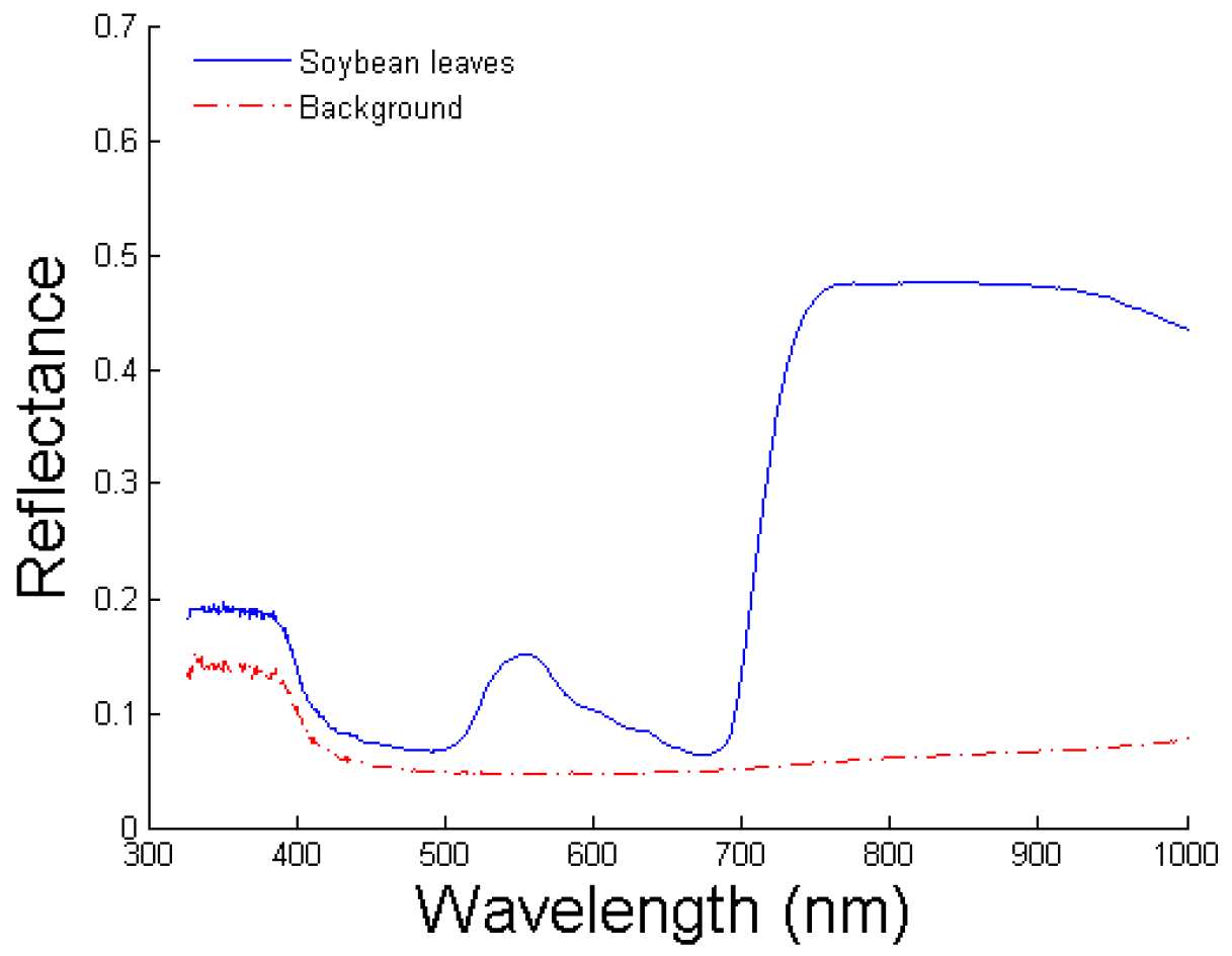
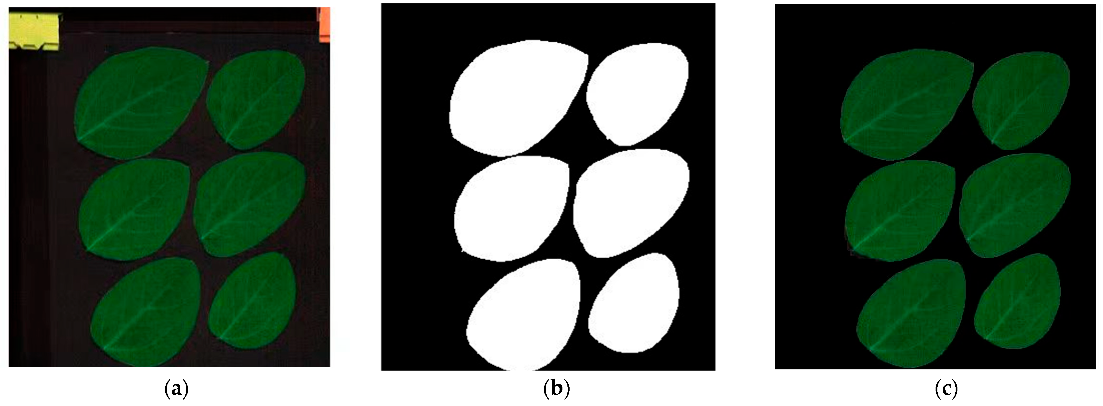
Since background information was included in the obtained hyperspectral imaging data of soybean leaves, a threshold segmentation algorithm has been used to separate the soybean leaves from the background area. There was a significant difference between the spectral reflectance of soybean leaves and the spectral reflectance of the background area (as shown in Figure 2). In the wavelength range of 300~500 nm, the spectral curve of soybean leaves was consistent with the change in the background spectral curve, and the difference in the two spectral reflectance curves was not obvious. With the increase in wavelength, the soybean leaves showed a typical green reflection peak near the wavelength range of 500~700 nm, which made the spectral curve of soybean leaves significantly different from the background. Especially in the vicinity of the 550 nm wavelength, the spectral reflectance curves of the soybean leaves and background were quite different. With the further increase in wavelength, the spectral reflectance curve of soybean leaves increased rapidly when the wavelength was greater than 700 nm; a typical near-infrared high-reflection platform of green plants appeared. The reflection platform maximized the difference in spectral reflectance between soybean leaves and the background. Therefore, the spectral values at 550 nm and 750 nm were used for threshold segmentation in this study. During the threshold segmentation, the segmentation threshold values at 550 nm and 750 nm were set to be 0.1 and 0.3, respectively. The raw hyperspectral images of soybean leaves are shown in Figure 3a. According to the set threshold value, the ENVI 5.3 software was used for binarization and mask processing to generate the binarization image of soybean leaves (as shown in Figure 3b) and the hyperspectral image of soybean leaf nitrogen content after background removal (as shown in Figure 3c).
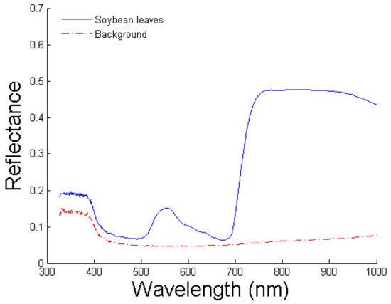
Figure 2.
Contrast of spectral curve between soybean leaves and background.
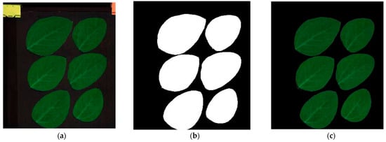
Figure 3.
Extracting hyperspectral images of soybean leaves: (a) raw hyperspectral images of soybean leaves; (b) binary image of soybean leaves after background removal; (c) hyperspectral images of soybean leaves after background removal.
3.2. Analysis of Spectral Reflectance of Soybean Leaves
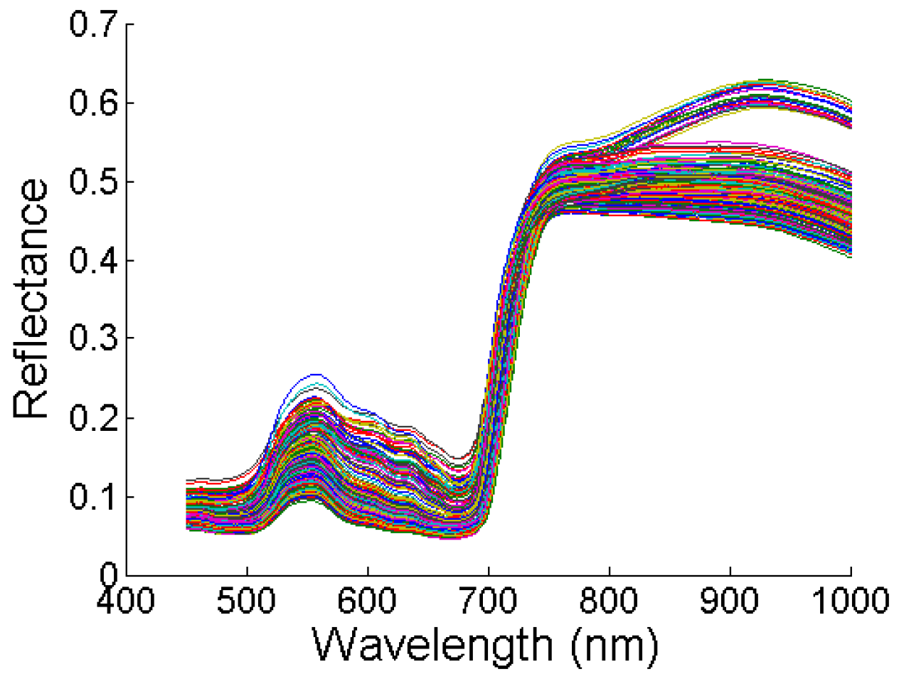
The average spectral value of all pixels in the soybean leaves after background separation was calculated, and the average spectral curves containing 707 bands were obtained (as shown in Figure 4). The spectral reflectance in the visible band was relatively low, and there was a typical plant chlorophyll reflection peak near 550 nm. This was because the spectral characteristics of the leaves in the visible light range were mainly affected by the pigments in the soybean leaves. The spectral absorption peaks of the pigments were mainly concentrated near the blue and red light bands, and the spectral absorption peaks were near the green light band. Therefore, the reflectance spectra of soybean leaves had two obvious absorption valleys near 450 nm and 670 nm, and a reflection peak near 550 nm. With the increase in wavelength, the spectral reflectance of soybean leaves increased sharply after 690 nm; a typical near-infrared high-reflection platform was formed. The spectral reflectance near the reflection platform was sensitive to the changes of vegetation nutrition, growth and water content [19]. The spectral reflectance after near-infrared high reflection was mainly affected by the internal structure of the leaves (such as leaf gap, cell thickness, and stomatal aperture, etc.). The level of spectral reflectance after high near-infrared reflectance was closely related to the number of leaf cell layers, the shape of the leaf cells, and the composition of the leaves.
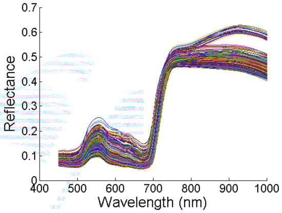
Figure 4.
Reflectance spectra of soybean canopy under different nitrogen content. The different colored lines in the figure represent the different spectral curves of the soybean samples.
3.3. Correlation Analysis between Spectral Reflectance and Leaf Nitrogen Content of Soybean Leaves
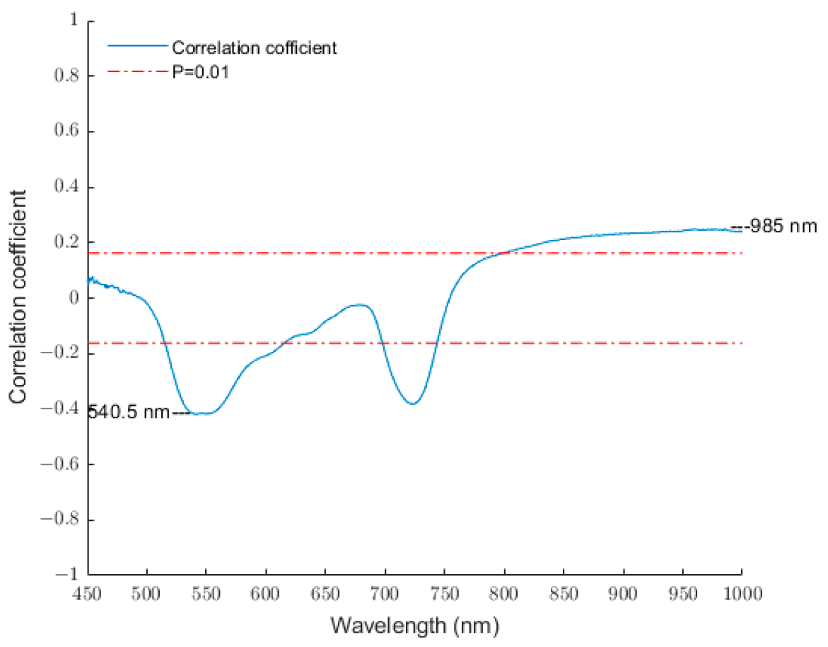
The correlation between soybean leaf spectral reflectance and leaf nitrogen content was analyzed, as shown in Figure 5. The spectral reflectance of soybean leaves was positively correlated with leaf nitrogen content in the spectral range of 450~494 nm and 755–1000 nm, while the spectral reflectance of soybean leaves was negatively correlated with leaf nitrogen content in the spectral range of 495~754 nm. In the positive correlation coefficient, the spectral reflectance of soybean leaves in the range of 798.8~1000 nm was significantly positively correlated with leaf nitrogen content (p < 0.01), and the maximum correlation coefficient was 0.2496 at 985 nm. In the negative correlation coefficient, the spectral reflectance of soybean leaves in the range of 516~615 nm and 698~774 nm was significantly negatively correlated with leaf nitrogen content (p < 0.01); the absolute value of the negative correlation coefficient between the spectral reflectance and the nitrogen content of soybean leaves was obtained at 540.5 nm, which was 0.4185. In addition, since the absolute value of the negative correlation coefficient was greater than the positive correlation coefficient, the negative correlation was mainly concentrated near the visible and near-infrared platforms. Therefore, the correlation between soybean leaf spectral reflectance and leaf nitrogen content in the visible band may be better than that in the near-infrared band.
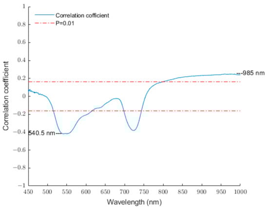
Figure 5.
Correlation curve between leaf spectra and leaf nitrogen content of the soybean. Note: The red dashed line represents the extreme significant level (p < 0.01). The blue solid curve is the correlation curve between leaf spectra and the leaf nitrogen content of the soybean.
3.4. Results of Full Spectral Models
The raw spectra and preprocessed spectra were used to build PLS model of soybean leaf nitrogen content. Table 3 showed the prediction results of established PLS models. Using the model evaluation index aforementioned, the established PLS prediction models were analyzed and evaluated. The performances of the PLS model established by 1-Der, 2-Der, SNV, MSC and SG were worse than that of the PLS model based on raw spectra. Among them, the PLS model established by the spectra of 2-Der preprocessed had the worst performance, with Rp2 of 0.9263, RMSEP of 2.8322 mg/g and RPD of 3.6945. While PLS models established by De-trending and DOSC had better performance compared with the raw spectra, and the performance of the PLS model established by DOSC was the best, with Rp2 of 0.9428, RMSEP of 2.4858 mg/g and RPD of 4.2092. The evaluation indexes Rp2, RMSEP and RPD of PLS model established by DOSC was 0.4987%, 0.5461% and 4.267% higher than by those of the PLC model established by raw spectra. In general, all the PLS models shown in Table 3 were ideal with Rp2 above 0.9, and RPD above 2.0, which indicated that the established PLS models could be used for the detection of the nitrogen content in soybean leaves. Since the PLS models established by full spectra (containing a large amount of redundant and uninformative information) were relatively complex (containing 707 variables), the DOSC preprocessing method had the best effect. Hence, the DOSC preprocessed spectra were used for further characteristic wavelength extraction to simplify the model.
Table 3.
Prediction results of the nitrogen content in soybean leaves with different pre-processing methods.
3.5. Selection of Characteristic Wavelength of Soybean Leaf Nitrogen Content
Spectral data of 707 bands contained a large amount of redundant, collinear and overlapping information, which deteriorated the performance of the multivariate calibration models. As discussed above, the PLS model with DOSC preprocessed spectra had the best performance. Therefore, the DOSC spectra were employed for the characteristic wavelength selection of the nitrogen content in soybean leaves. In this study, SPA, GA and RF were used to select characteristic wavelengths with the smallest collinearity and the largest correlation for improving the modeling efficiency.
When selecting the characteristic wavelengths of soybean leaf nitrogen content by SPA, the maximum number of variables was set to 50, and the optimal numbers of characteristic wavelengths were determined according to the minimum value of RMSECV. As is shown in Figure 6, the RMSE value was 2.575, and the number of characteristic wavelengths selected by SPA was the best, which was 26. These characteristic wavelengths were distributed near the band of green light (550 nm), near-infrared platform (700 nm) and near-infrared (980 nm).
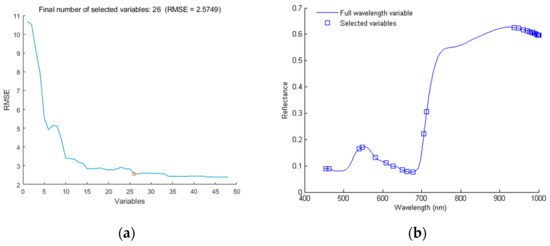
Figure 6.
Selection process of characteristic wavelengths for nitrogen content in soybean leaves based on SPA algorithm: (a) change in RMSECV value with an increase in modeling variables; (b) distribution of characteristic wavelengths extracted by SPA cited. Note: The red box in subfigure (a) represents the number of modelling variables selected by the SPA algorithm.
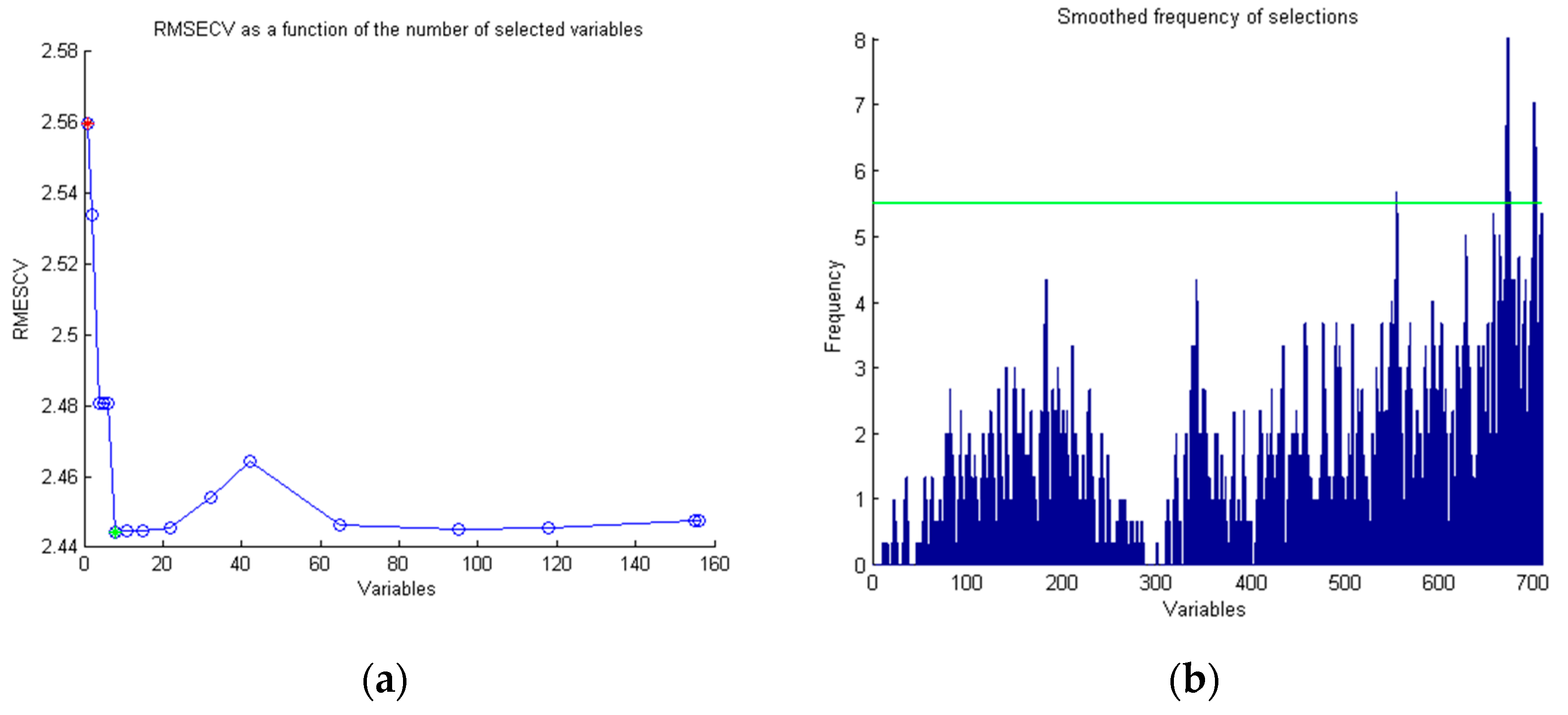
The parameters of the GA algorithm were set as follows: the initial population was 30, the probability of chromosome crossover was 50%, the probability of chromosome mutation was 1%, the maximum principal component score was 15, the window-smoothing width was 3, the number of iterations was 200, and the fitness function was RMSECV. The specific process of selecting characteristic wavelengths by GA was illustrated in Figure 7. According to the variable selection principle similar to the SPA algorithm, namely the optimal numbers of characteristic wavelengths were determined based on the minimum value of RMSECV. The minimum RMSECV value appeared when the number of modeling variables was 7 (as shown in Figure 7a). Therefore, the number of characteristic wavelengths selected by GA algorithm was 7, and the corresponding frequency selection threshold was 5.5 (as shown in Figure 7b).
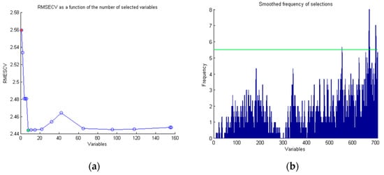
Figure 7.
Selection process of characteristic wavelengths for nitrogen content in soybean leaves based on GA algorithm: (a) change in RMSECV value with an increase in modeling variables; (b) selected frequency of characteristic wavelengths based on GA algorithm. Note: The red plus sign in subfigure (a) represents the RMSECV value corresponding to having one modelling variables, and the green dot in subfigure (a) represents the number of modelling variables corresponding to the minimum RMSECV value. The green line in subfigure (b) is the variable selection probability corresponding to the minimum value of RMAECV in subfigure (a).
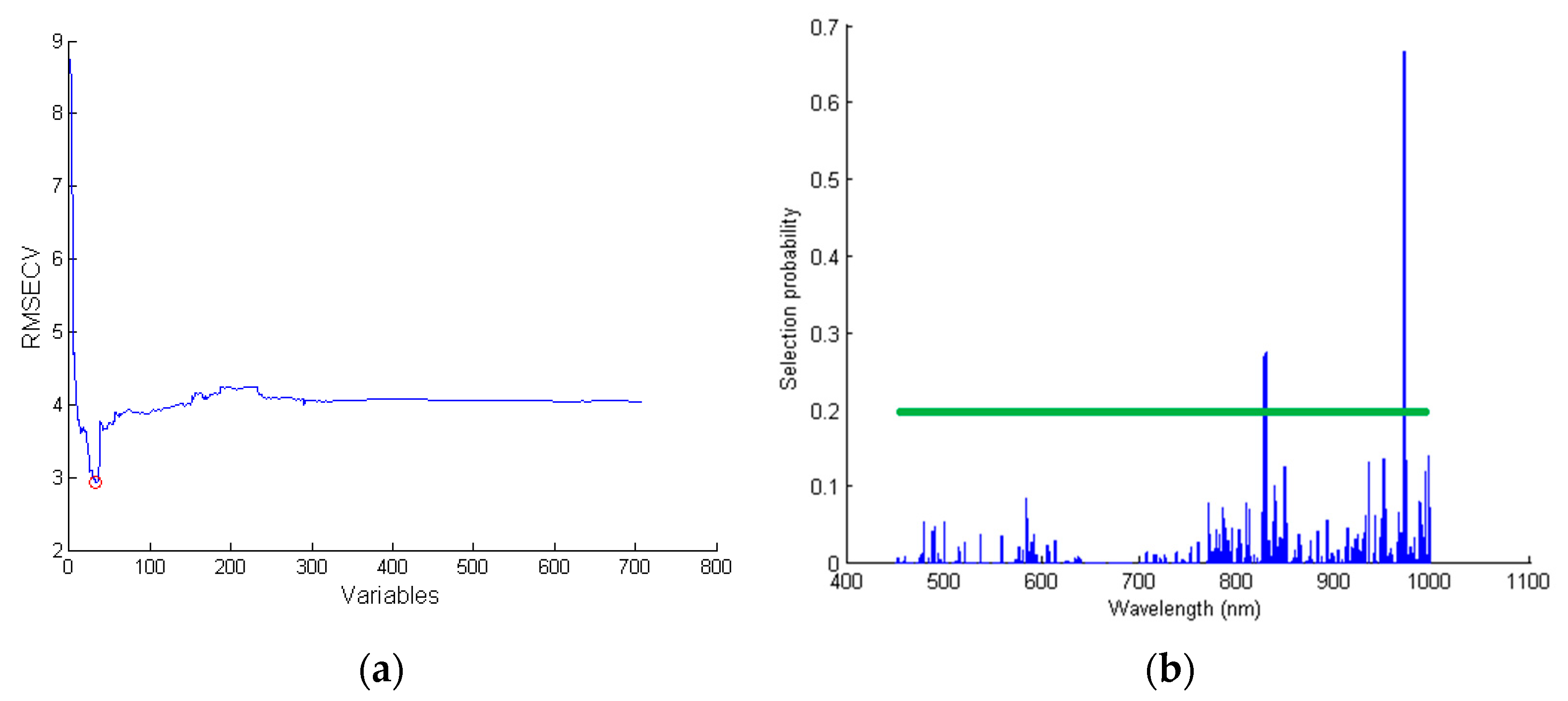
When the RF algorithm was employed to extract the characteristic wavelengths, the number of initial frogs and iterations was set to 5 and 1000, respectively, and the maximum principal component score was 10. The principle of variable selection was similar to the SPA algorithm. Figure 8a shows the change in RMSECV value along with the number of modeling variables, which was computed by the RF algorithm. The minimum RMSECV value appeared when the number of modeling variables was 5. The corresponding variable selection probability was greater than 0.2 (as shown in Figure 8b).
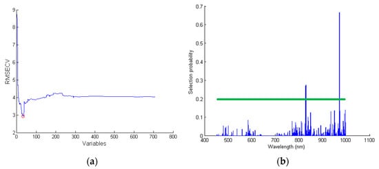
Figure 8.
Selection process of characteristic wavelengths for nitrogen content in soybean leaves based on RF algorithm: (a) change in RMSECV value with an increase in modeling variables; (b) selection probability of characteristic wavelengths based on RF algorithm. Note: The green line in subfigure (b) is the variable selection probability corresponding to the minimum value of RMAECV in subfigure (a).
The distribution of characteristic wavelengths related to the nitrogen content in soybean leaves was selected by the SPA, GA and RF algorithms, as shown in Figure 9. The characteristic wavelengths selected by the SPA algorithm were near the visible light, near-infrared reflection platform and near-infrared band, while the characteristic wavelengths selected by the RF and GA algorithms were mainly concentrated in the near-infrared band, which indicated that the spectral information in the near-infrared band may contain more information related to the nitrogen content of soybean leaves.
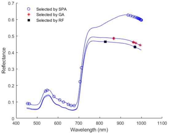
Figure 9.
Specific position distribution of characteristic wavelengths selected by SPA, GA, and RF algorithms.
3.6. Results of Full Spectral Models
In order to compare the effectiveness of the SPA, GA, and RF algorithms, the prediction models for the nitrogen content in soybean leaves were developed with PLS combined with the characteristic wavelengths selected before. The results of the established PLS models were presented in Table 4. The PLS models established by characteristic wavelengths selected by SPA algorithms were slightly worse than the full spectra (DOSC preprocessed, 707 variables), with Rc2 of 0.9184 and Rp2 of 0.9413,RPD of 4.078, RMSEC of 2.5047 and RMSEP of 2.5654. While the performance of the PLS models established by characteristic wavelengths, which were selected by the GA and RF algorithms, were better than the performance established by optimal full spectra (DOSC preprocessed, 707 variables). Among them, the model established based on the five characteristic wavelengths selected by the RF algorithm provided the best performance with higher Rc2 (0.9261), Rp2 (0.9466), and RPD (4.3536), and lower RMSEC (2.4858) and RMSEP (2.4034). This was because the information about redundant and collinear wavelengths that existed in the full spectra was eliminated by the GA and RF algorithms, and the wavelengths, which were closely related to the nitrogen content in soybean leaves, remained. As discussed above, the evaluation indicators of the model established by the characteristic wavelengths extracted by the RF algorithm were the best, and the number of characteristic wavelengths contained 7 variables, which was 0.707% of the full wavelength variable. Therefore, the RF algorithm was the most suitable method for selecting the characteristic wavelengths of soybean leaf nitrogen content.
Table 4.
Prediction results of PLS models with different characteristic variable selection algorithms for the nitrogen content of soybean leaves.
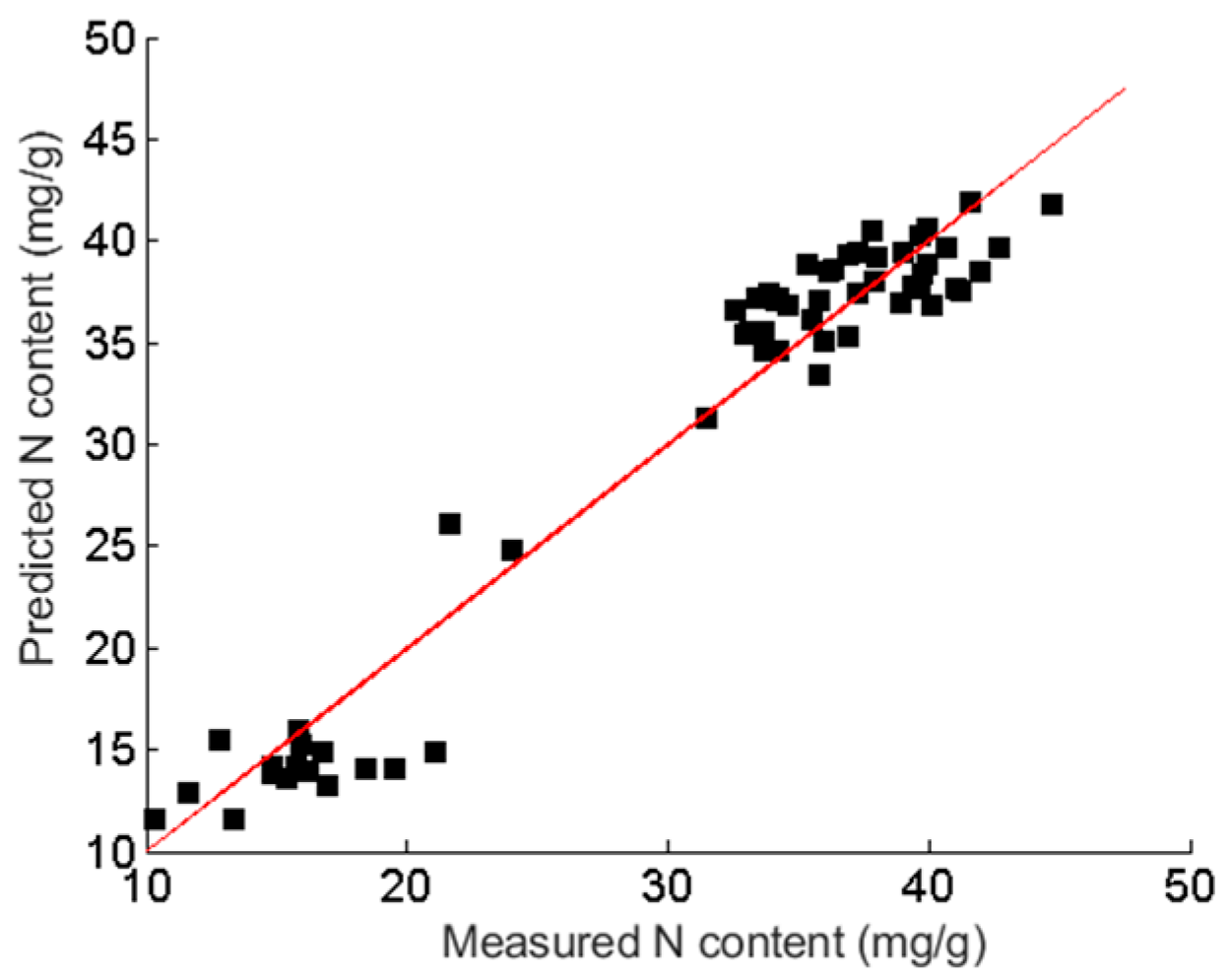
Figure 10 showed the scatter plots of the measured nitrogen content and predicted nitrogen content generated by the DOSC-RF-PLS model. The samples of the prediction set were distributed near the 1:1 line. It indicated that the predicted value of the nitrogen content in soybean leaves had a good correlation with the measured value, and the established prediction model had good accuracy. The 5 characteristic wavelengths (827.262 nm, 828.844 nm, 969.166 nm, 969.959 nm and 970.752 nm) selected by the RF algorithm not only simplified the complexity of the soybean leaf nitrogen content detection model, but also reduced the modeling time. In addition, these selected characteristic wavelengths can also provide data and method support for the development of rapid detection equipment for the nitrogen content in soybean leaves.
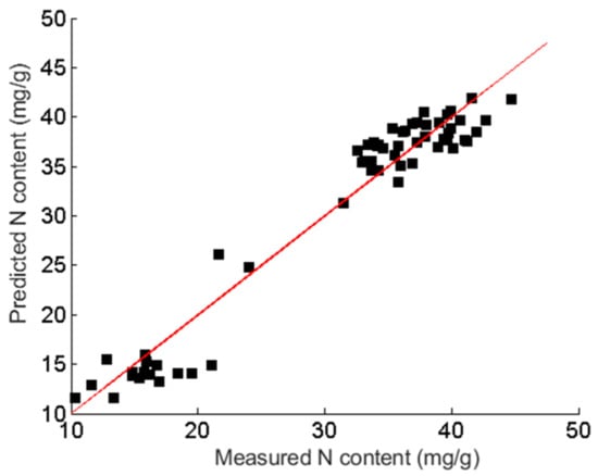
Figure 10.
Prediction results of the nitrogen content of soybean leaves by the DOSC-RF-PLS model.
3.7. Visualization of Nitrogen Content Distribution in Soybean Leaves
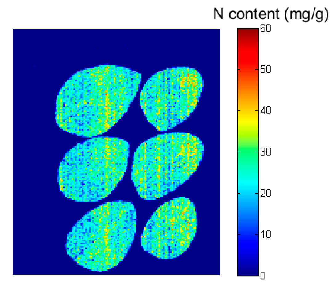
Based on the discussion above, the DOSC-RF-PLS model was the optimal prediction model for the nitrogen content of soybean leaves. Thus, the spatial distributions of the nitrogen content in soybean leaves were generated in a pixel manner using the DOSC-RF-PLS model. Firstly, the nitrogen content values corresponding to each pixel in the hyperspectral image of the soybean leaves (after background removal) were calculated to generate the grayscale distribution maps of the nitrogen content using the DOSC-RF-PLS model. Afterwards, pseudo-color processing was performed on the generated grayscale spatial distribution data of the nitrogen content in soybean leaves, and, finally, visual distribution maps of the nitrogen content were obtained (as shown in Figure 11). Figure 11 is the distribution map of the estimated nitrogen content. The dark blue area around the leaves in Figure 11 represents the background, and the different colors and their depths in the leaves represent different nitrogen content values. The color band on the right side of Figure 11 shows the distribution range of the nitrogen content corresponding to different colors. The blue color represents a lower nitrogen content value. With an increase in the nitrogen content value in soybean leaves, the color gradually changes and becomes yellow. As the nitrogen content value increases, it eventually becomes red.
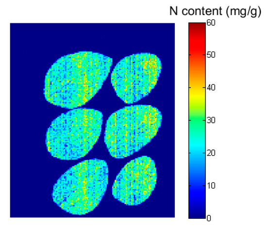
Figure 11.
Distribution of the nitrogen content of soybean leaves.
The distribution of the nitrogen content in the soybean leaves is clearly shown in Figure 11. Different colors on the same leaf represent different biochemical components contained in soybean leaves; this is mainly reflected in the fact that some areas on one leaf are bluer (bluer areas represent lower nitrogen content), while some areas on the leaf are yellower (yellower areas represent higher nitrogen content). This indicates that the distribution of the nitrogen content in the leaves is uneven. This is because the difference in the nitrogen content in the same leaf was mainly caused by the difference in leaf nutrient composition. In addition, due to the different physiological structures of different parts of the leaves, there were some differences in the spatial distribution of the leaf nitrogen content. The spatial differences of the components shown by hyperspectral imaging technology were also reflected in the soluble solids and sugar content of crops such as potatoes and sweet potatoes [20,21,22]. This showed that hyperspectral imaging technology was an effective tool for the detection of the nitrogen content in soybean leaves and its spatial distribution analysis, and that the tool provided decision-making basis for the effective monitoring and fertilization management of soybean nutrition.
4. Discussion
In the detection of plant nutrient information, traditional crop nutrient diagnostic methods have some shortcomings in the detection of nutrient information. For instance, the appearance diagnosis method is subjective, easy to misdiagnose, and cannot realize the effect of active prevention [23,24]. The chemical diagnosis method has poor timeliness, complex operation, and high destructiveness [25,26]. The chlorophyll meter diagnosis method has a small detection range, high environmental requirements, and cannot accurately detect the nutrient status of a larger area [27]. Therefore, the traditional nutrient diagnostic methods have great limitations and latency in practical applications, and cannot adapt to the practical needs of precision agriculture for the rapid, real-time, nondestructive, and large-area detection of crop nutrient information. In this paper, we proposed a method for detecting the nitrogen content of soybean leaves based on hyperspectral imaging technology, with a high detection accuracy of Rp2 of 0.9466. The nitrogen content of soybean leaves can be detected in a rapid, real-time and non-destructive manner, which could provide scientific guidance for the monitoring of nutrient dynamics and the reasonable regulation of fertilizers in the process of soybean production.
In the aspect of model accuracy, Kang Kai et al. used multispectral techniques to detect the nitrogen content of canopy leaves in soybean fields, and the coefficient of determination R² of the established regression model ranged from 0.8 to 0.9 [28]. Wang Lifeng et al. developed a 1st-SPA-PLS model for monitoring the nitrogen content of corn leaves in the field using hyperspectral imaging technology, with an accuracy of Rp2 of 0.749 [29]. Qin Zhanfei et al. estimated the total nitrogen content of rice leaves in the yellow diversion irrigation area using hyperspectral imaging technology, and the modeling accuracy R² was 0.673 [30]. The accuracy of the soybean leaf nitrogen content detection model established in this study was slightly higher than that of the nitrogen content detection models established in other studies. On the one hand, it is probable that the greenhouse potting method was used for fertilizer control in this study, and the control of the nitrogen fertilizer gradient is relatively accurate and stable. On the other hand, it may be that indoor hyperspectral imaging data acquisition was stable compared with the outdoor field measurement environment, with relatively small interfering factors and noise signals; therefore, the stability and reliability of the established nitrogen content detection model were higher. In addition, most of the research data collection for nitrogen content detection focused on one or fewer fertility stages due to the great differences in the nutrient composition of the crop at different growth stages; the experimental samples obtained at one or more fertility stages had a small nitrogen gradient, whereas the nitrogen detection in this study was carried out throughout the whole fertility stage of the soybean, and it was possible to obtain samples of the soybean leaves with large nitrogen gradients, which may be another important reason for the slightly higher accuracy of the nitrogen content detection model established in this study than that of the others.
5. Conclusions
- (1)
- The correlation between the spectral reflectance of soybean leaves and the leaf nitrogen content was analyzed. It was found that the correlation coefficient between soybean leaf spectral reflectance and leaf nitrogen content in the range of 798.8~1000 nm reached a very significant positive correlation level (p < 0.01), and the spectral reflectance of soybean leaves in the range of 516~615 nm and 698~774 nm was significantly negatively correlated with the leaf nitrogen content (p < 0.01). Among them, the maximum positive correlation coefficient was 0.2496 at 985 nm, and the maximum absolute value of the negative correlation coefficient of spectral reflectance was 0.4185 at 540.5 nm.
- (2)
- The performances of seven spectral preprocessing methods on the prediction of the nitrogen content in soybean leaves were compared. The PLS model combined with spectra preprocessed by DOSC had the best performance among the full-spectra models, and its Rc2 was 0.9233, RMSEC was 2.4286, Rp2 was 0.9428, RMSEP was 2.4858, and RPD was 4.2092. Therefore, the DOSC preprocessing method was selected as the best preprocessing method for the detection of the nitrogen content in soybean leaves.
- (3)
- SPA, GA and RF algorithms were employed to select the characteristic wavelengths, which were closely related to the nitrogen content in soybean leaves. The five characteristic wavelengths, including 827.262 nm, 828.844 nm, 969.166 nm, 969.959 nm and 970.752 nm selected by the RF algorithm had the best prediction effect for the prediction of the nitrogen content in soybean leaves combined with the PLS model, and its Rp2, RMSEP and RPD were 0.9261, 2.4034 and 4.3536, respectively. The selection of characteristic wavelengths not only compressed the spectral data, but also improved the prediction effect of the model. This was helpful for the development of portable detection equipment for the soybean leaf nitrogen content.
- (4)
- The visual distribution map of the nitrogen content in soybean leaves was generated using the DOSC-RF-PLS model, which was considered to be the optimal prediction model for the nitrogen content in soybean leaves. The map provided the basis for analyzing the spatial distribution difference of the nitrogen content in soybean leaves. The overall results in this study showed that hyperspectral imaging technology was an effective tool for soybean leaf nitrogen content detection and spatial distribution analysis, and provided decision-making basis for the effective monitoring of soybean nutrition and fertilization management.
Author Contributions
Conceptualization, Y.Z. Conceptualization, Y.Z. and T.L.; methodology, Y.Z. and M.G.; supervision, L.W. and F.Z.; validation, M.G.; formal analysis, Y.Z. and M.G.; investigation, L.W., X.C. and T.L.; resources, Y.Z. and F.Z.; data curation, Y.Z., M.G. and T.L.; writing—original draft preparation, Y.Z.; writing—review and editing, Y.Z., M.G., X.C. and L.W.; visualization, Y.Z.; project administration, Y.Z. and X.C.; funding acquisition, Y.Z. All authors have read and agreed to the published version of the manuscript.
Funding
This research was funded by the Henan Provincial Science and Technology Research Project (No. 212102110207, No. 2102110159, No. 242102110337), 2023 Henan Science and Technology Commissioner Project, Collaborative Education Project of Ministry of Education (No.220505078205656, No.220503880205011), and the National Natural Science Foundation of China (No. 32202096).
Data Availability Statement
Data are contained within the article.
Acknowledgments
The authors would like to thank the editor and reviewers for their assistance and valuable comments.
Conflicts of Interest
The authors declare no conflicts of interest.
References
- Savary, S.; Willocquet, L.; Pethybridge, S.J.; Esker, P.; McRoberts, N.; Nelson, A. The global burden of pathogens and pests on major food crops. Nat. Ecol. Evol. 2019, 3, 430–439. [Google Scholar] [CrossRef] [PubMed]
- Bureau of Statistics of the China. China Statistical Yearbook; China Statistics Press: Beijing, China, 2022. [Google Scholar]
- Zhang, Y.K.; Luo, B.; Pan, D.Y.; Song, P.; Lu, W.C.; Wang, C.; Zhao, C.J. Estimation of Canopy Nitrogen Content of Soybean Crops Based on Fractional Differential Algorithm. Spectrosc. Spectr. Anal. 2018, 38, 3221–3230. [Google Scholar]
- Pandey, P.; Payn, K.G.; Lu, Y.; Heine, A.J.; Walker, T.D.; Acosta, J.J.; Young, S. Hyperspectral imaging combined with machine learning for the detection of fusiform rust disease incidence in loblolly pine seedlings. Remote Sens. 2021, 13, 3595. [Google Scholar] [CrossRef]
- Ren, Y.; Sun, D. Monitoring of moisture contents and rehydration rates of microwave vacuum and hot air dehy-drated beef slices and splits using hyperspectral imaging. Food Chem. 2022, 382, 132346. [Google Scholar] [CrossRef] [PubMed]
- Mishra, P.; Asaari, M.S.M.; Herrero-Langreo, A.; Lohumi, S.; Diezma, B.; Scheunders, P. Close range hyperspectral imaging of plants: A review. Biosyst. Eng. 2017, 164, 49–67. [Google Scholar] [CrossRef]
- Gowen, A.; Odonnell, C.; Cullen, P.; Downey, G.; Frias, J. Hyperspectral imaging—An emerging process analytical tool for food quality and safety control. Trends Food Sci. Technol. 2007, 18, 590–598. [Google Scholar] [CrossRef]
- Zhu, H.C.; Liu, H.Y.; Xu, Y.X.; Guijun, Y. UAV-based hyperspectral analysis and spectral indices constructing for quantitatively monitoring leaf nitrogen content of winter wheat. Appl. Opt. 2018, 57, 7722–7732. [Google Scholar] [CrossRef] [PubMed]
- Goel, P.; Prasher, S.; Landry, J.; Patel, R.; Bonnell, R.; Viau, A.; Miller, J. Potential of airborne hyperspectral remote sensing to detect nitrogen deficiency and weed infestation in corn. Comput. Electron. Agric. 2003, 38, 99–124. [Google Scholar] [CrossRef]
- Zhang, X.L.; Liu, F.; Nie, P.C.; He, Y.; Bao, Y.D. Rapid detection of nitrogen content and distribution in oilseed rape leaves based on hyperspectral imaging. Spectrosc. Spectr. Anal. 2014, 34, 2513. [Google Scholar]
- Zou, X.; Shi, J.; Hao, L.; Zhao, J.; Mao, H.; Chen, Z.; Li, Y.; Holmes, M. In vivo, noninvasive detection of chlorophyll distribution in cucumber (Cucumis sativus) leaves by indices based on hyperspectral imaging. Anal. Chim. Acta 2011, 706, 105–112. [Google Scholar]
- Wang, H.; Peng, J.; Xie, C.; Bao, Y.; He, Y. Fruit Quality Evaluation Using Spectroscopy Technology: A Review. Sensors 2015, 15, 11889–11927. [Google Scholar] [CrossRef] [PubMed]
- Pu, H.B.; Kamruzzaman, M.; Sun, D.W. Selection of feature wavelengths for developing multispectral imaging systems for quality, safety and authenticity of muscle foods—A review. Trends Food Sci. Technol. 2015, 45, 86–104. [Google Scholar] [CrossRef]
- Li, X.; Jiang, H.; Jiang, X.; Shi, M. Identification of Geographical Origin of Chinese Chestnuts Using Hyperspectral Imaging with 1D-CNN Algorithm. Agriculture 2021, 11, 1274. [Google Scholar] [CrossRef]
- Nagasubramanian, K.; Jones, S.; Sarkar, S.; Singh, A.K.; Singh, A.; Ganapathysubramanian, B. Hyperspectral band selection using genetic algorithm and support vector machines for early identification of charcoal rot disease in soybean stems. Plant Methods 2018, 14, 86. [Google Scholar] [CrossRef] [PubMed]
- Eusuff, M.M.; Lansey, K.E.; Lansey, K. Optimization of Water Distribution Network Design Using the Shuffled Frog Leaping Algorithm. J. Water Resour. Plan. Manag. 2003, 129, 210–225. [Google Scholar] [CrossRef]
- Orrillo, I.; Cruz-Tirado, J.P.; Cardenas, A.; Oruna, M.; Carnero, A.; Barbin, D.F.; Siche, R. Hyper-spectral imaging as a powerful tool for identification of papaya seeds in black pepper. Food Control 2019, 101, 45–52. [Google Scholar] [CrossRef]
- Kamruzzaman, M.; Elmasry, G.; Sun, D.W.; Allen, P. Prediction of some quality attributes of lamb meat using near-infrared hy-perspectral imaging and multivariate analysis. Anal. Chim. Acta 2012, 714, 57–67. [Google Scholar] [CrossRef]
- Gao, Z.; Luo, N.; Yang, B.; Zhu, Y. Estimating Leaf Nitrogen Content in Wheat Using Multimodal Features Extracted from Canopy Spectra. Agronomy 2022, 12, 1915. [Google Scholar] [CrossRef]
- Kjær, A.; Nielsen, G.; Stærke, S.; Clausen, M.R.; Edelenbos, M.; Jørgensen, B. Prediction of Starch, Soluble Sugars and Amino Acids in Potatoes (Solanum tuberosum L.) Using Hyperspectral Imaging, Dielectric and LF-NMR Methodologies. Potato Res. 2016, 59, 357–374. [Google Scholar] [CrossRef]
- Rady, A.; Guyer, D. Evaluation of sugar content in potatoes using NIR reflectance and wavelength selection techniques. Postharvest Biol. Technol. 2015, 103, 17–26. [Google Scholar] [CrossRef]
- Shao, Y.Y.; Liu, Y.; Xuan, G.T.; Wang, Y.X.; Gao, Z.M.; Hu, Z.C.; Han, X.; Gao, C.; Wang, K.L. Application of hyperspectral imaging for spatial prediction of soluble solid content in sweet potato. RSC Adv. 2020, 10, 33148–33154. [Google Scholar] [CrossRef] [PubMed]
- Liu, Z.Y. Review and prospect of plant nutrition diagnosis. Soils 1990, 22, 173–176. [Google Scholar]
- Jiang, Y.M. Study on Mineral Nutrition Characteristics, Nutrition Diagnosis and Fertilization of Red Fuji Apple; China Agricultural University: Beijing, China, 2001. [Google Scholar]
- Card, D.H.; Peterson, D.L.; Matson, P.A.; Aber, J.D. Prediction of leaf chemistry by the use of visible and near infrared re-flectance spectroscopy. Remote Sens. Environ. 1988, 26, 123–147. [Google Scholar] [CrossRef]
- Turner, F.T.; Jund, M.F. Assessing the nitrogen requirements of rice crops with a chlorophyll meter. Aust. J. Exp. Agric. 1994, 34, 1001–1005. [Google Scholar] [CrossRef]
- Schepers, J.S.; Francis, D.D.; Vigil, M.; Below, F.E. Comparison of corn leaf nitrogen concentration and chlorophyll meter readings. Commun. Soil Sci. Plant Anal. 1992, 23, 2173–2187. [Google Scholar] [CrossRef]
- Kang, K.; Zhang, W.; He, Y.; Qi, L.Q.; Zhang, P. Detection of nitrogen content in soybean canopy leaves based on UAV multi-spectral images. Agric. Mech. Res. 2024, 46, 151–156. [Google Scholar]
- Wang, L.F.; Zhang, C.L.; Zhao, Y.; Song, Y.Z.; Wang, R.T.; Su, Z.B.; Wang, S.W. Detection model of nitrogen content in maize leaves by hyperspectral imaging technology. Agric. Mech. Res. 2017, 39, 140–147. [Google Scholar]
- Qin, Z.F.; Chang, Q.R.; Xie, B.N.; Shen, J. Estimation of total nitrogen content in rice leaves in Yellow River irrigation area based on UAV hyperspectral image. Acta Agric. Eng. Sci. 2016, 32, 77–85. [Google Scholar]


Disclaimer/Publisher’s Note: The statements, opinions and data contained in all publications are solely those of the individual author(s) and contributor(s) and not of MDPI and/or the editor(s). MDPI and/or the editor(s) disclaim responsibility for any injury to people or property resulting from any ideas, methods, instructions or products referred to in the content. |
© 2024 by the authors. Licensee MDPI, Basel, Switzerland. This article is an open access article distributed under the terms and conditions of the Creative Commons Attribution (CC BY) license (https://creativecommons.org/licenses/by/4.0/).