NDVI Prediction of Mediterranean Permanent Grasslands Using Soil Moisture Products

Abstract

Vegetation indices are widely used to assess vegetation dynamics. The Normalized Vegetation Index (NDVI) is the most widely used metric in agriculture, frequently as a proxy for different physiological and agronomical aspects, such as crop yield or biomass, crop density, or drought stress. Much effort has therefore been directed to NDVI forecasting, which is usually correlated with precipitation. However, in Mediterranean and arid climates, the relationship is more complex due to prolonged dry periods and sparse precipitation events. In this study, we forecast the NDVI 7 and 30 days ahead for Mediterranean permanent grasslands using a machine learning Random Forest (RF) model for the period from 2015 to 2022. The model compares two soil moisture products as predictors: simulated soil moisture values based on in situ soil moisture sensor observations and remote sensing-derived observations of Soil Water Index (SWI) values. We further analyzed the anomalies of the predicted NDVI using the z-score. The results show that both products can be used as reliable predictors for permanent grasslands in Mediterranean areas. Predictions at 7 days are more accurate and better forecast the negative effect of drought on vegetation dynamics than those at 30 days. This study shows the potential of using a simple methodology and readily available data to predict the grassland growth dynamics in the Mediterranean area.

1. Introduction

Savanna-like agroforestry systems cover about 3.5 million hectares in Mediterranean Europe and about 1 million hectares in North Africa [1,2]. This land use is composed of scattered oak trees (Quercus rotundifolia), and permanent grassland (unrenewed herbage layer of 5 or more years) for livestock grazing [2]. In the Iberian peninsula, savanna-like systems are called Dehesa in Spain and Montado in Portugal; these names refer to the fact that the land is divided into large plots bordered by stone walls, where rotational grazing (rangeland) is practiced [2]. Grassland ecosystems play an important role in sustaining the economy of marginal lands in the Mediterranean through livestock production and in preserving their endemic biodiversity and cultural heritage [3]. Drought is a severe natural event with a gradual onset, vast impact range, long duration, and the potential to recur frequently within short periods, resulting in significant losses. As global warming progresses, the frequency of droughts has been notably increasing [4,5]. Most regions worldwide experience droughts, particularly arid areas, where annual rainfall is limited to a few events. The impact of drought on vegetation is profound, as it influences the thermal inertia of the soil and atmosphere, surface temperature, soil moisture, and rainfall, among other environmental factors. Satellite-based indices have proven effective in detecting and identifying drought conditions globally [6,7,8]. Mediterranean grasslands are especially vulnerable to drought. These ecosystems are heavily influenced by climatic factors such as precipitation and temperature, which control the soil moisture content and vegetation growth [9,10]. Indeed, in the Mediterranean climate, grassland production is limited due to frequent long, dry summers, which cause severe crop yield drops and, hence, important economic losses. This susceptibility of Mediterranean grasslands to drought is increasingly exacerbated by climate change [11]. Therefore, accurate forecasts of grassland yield, particularly during dry periods, are crucial for both farmers and policymakers to apply mitigation measures and, hence, ensure food security [12]. In recent years, the integration of earth observation technologies has significantly advanced the field of environmental monitoring. Researchers have leveraged the Sentinel-1 and Sentinel-2 EO data, as well as innovative machine learning techniques, to address critical challenges in water resource management, crop growth assessment, and long-term ecological studies. Numerous quantitative techniques have been suggested and used to examine the dynamics and distribution of soil moisture across various scales. Soil moisture can be determined through two primary techniques: direct and indirect methods. The gravimetric method is the most accurate for measuring soil surface moisture in direct soil moisture estimation. This technique involves physically extracting a soil sample, drying it to remove moisture, and then weighing it to determine the moisture content. Although it provides precise measurements, the gravimetric method is labor-intensive, expensive, complex, and potentially destructive to the sampling site [13]. Indirect methods, such as time domain reflectometry (TDR) and frequency domain reflectometry (FDR), offer accurate soil moisture measurements without the need for sample extraction. These techniques involve sending electromagnetic waves into the soil and measuring the reflected signals to determine moisture content. TDR and FDR are known for their high temporal resolution and ability to provide direct measurements at various depths. However, their spatial representation is limited, which can be a significant drawback for large-scale studies [14,15]. Emerging technologies, such as cosmic-ray neutron sensing (CRNS) and global positioning system (GPS) techniques, partially address the spatial representation issue. CRNS measures soil moisture by detecting changes in the neutron flux emitted from the soil, providing a non-invasive and large-scale moisture estimation. Several studies have shown that CRNS maintains accuracy comparable to point sensors even under adverse conditions. GPS-based methods utilize signal reflections from the ground to estimate soil moisture, offering another innovative approach to large-scale soil moisture monitoring [16]. Using SSM estimating instruments presents specific advantages, including portability, ease of installation, operation, and maintenance, and the relative maturity of the technologies. These instruments can provide high temporal resolution and direct measurements at various depths. However, the challenges associated with these methods include their labor-intensive nature, high cost, complexity, and potential destructiveness, particularly in the case of gravimetric sampling. Despite these challenges, the ongoing development and integration of new technologies continue to enhance the accuracy and applicability of soil moisture measurement techniques [17].

Efremova et al. [18] conducted a study focusing on efficient soil moisture content (SMC) mapping using Sentinel-1 and Sentinel-2 data. Their methodology, employing a cycle-consistent adversarial network (CycleGAN) for time-series gap filling, demonstrated promising results in vineyards in South Australia’s Eden Valley. The use of Random Forest (RF) algorithms outperformed other machine learning models, showcasing the potential for accurate and real-time SMC predictions. Wentao Yu et al. [19] delved into the prediction of vegetation properties using deep recurrent neural networks with long short-term memory and gated recurrent units. Their models proved highly accurate in predicting vegetation indices based on historical observations from MODIS and Sentinel-2 data. The pixel-based models exhibited superior performance compared with traditional models, offering precise predictions across different regions, vegetation types, and growing seasons. Geng et al. [20] introduced an innovative approach aimed at prolonging the temporal coverage of soil moisture (SM) products by employing an artificial neural network in conjunction with MODIS optical products. Their method proved to be viable in regions characterized by moderate vegetation cover, offering a valuable resource for extensive ecological and hydrological studies over extended periods. The resulting long-term SM products exhibited a robust correlation with on-site measurements, underscoring the capability of this approach to contribute to the improvement of global water cycle studies. Tong et al. [21] addressed the significant gaps in Soil Moisture Active Passive (SMAP) data over the Tibetan Plateau. They proposed two methods: a machine learning technique using a Random Forest algorithm and a geostatistics technique employing ordinary kriging. Both methods demonstrated high correlation with official SMAP SM products, indicating their potential to fill gaps and to reconstruct complete SM data over this critical region. The results were cross-validated, showing robust performance with low root mean square error (RMSE) values.

Different methods have been developed for predicting grassland dynamics and yield using weather forecasting. McDonnel et al. [22], attempted 1- and 6-day forecasts of the grassland dynamics using management inputs, such as fertilizer application, and weather inputs, such as temperature and precipitation. Trnka et al. [23] developed an accurate grassland growth model, including not only the weather and the fertilizer application as inputs, but also the soil moisture balance. The benefit of using soil moisture information is that it integrates weather, evapotranspiration, plant-available water and, hence, vegetation state information. Indeed, soil moisture is an essential driver of grassland dynamics; it can explain up to 60% of the grassland yield variability and, when considered in productivity models, greatly improve model performance [24]. In the literature, vegetation dynamics are commonly monitored by remote sensing techniques, and, in particular, by using the Normalized Difference Vegetation Index (NDVI). NDVI is a simple indicator of the vegetation greenness, and it is widely applied to estimate vegetation density and crop yields [25,26]. Notably, in Spain, the NDVI is used for agricultural insurance purposes to quantify grassland yield losses during the growing season (October–June) and compensations due to drought or extreme weather conditions [27]. Previous studies have shown that the NDVI can be estimated from soil conditions; in particular, they show a good correlation in dry climates [28]. For instance, Chen et al. [29] found a good correlation between soil moisture and the NDVI in Australia’s mainland, observing that the highest positive correlations occur when the soil moisture precedes the NDVI by one month. Inland, however, where the tree cover is denser, soil moisture and the NDVI are positively correlated over a range of temporal scales (lag time from 0 to 5 months). In climates characterized by prolonged dry seasons, such as in southern Spain, the NDVI has shown to be better correlated with soil moisture than precipitation [30]. In the particular case of grassland areas, Wang et al. [31] found a better correlation in semi-arid than humid regions of the USA.

Previous studies have shown the potential of using the NDVI to support grazing and harvesting planning; in particular, using NDVI predictions to anticipate water deficiencies and, hence, yield losses [32]. One approach to predict the NDVI is by using autoregressive models, i.e., to forecast future NDVI values using a linear combination of past NDVI values. This approach has shown high reliability in forestry land uses, mainly thanks to plant growth seasonality [33]. Another approach not based on the use of past data is the use of seasonal weather forecasts. Iwasaki [34] tried to predict the NDVI distribution in an arid climate for 1–3 months using a seasonal weather forecast. They showed an especially weak prediction efficiency and advised against the use of precipitation forecasts for NDVI prediction in dry regions. Considering the NDVI as a proxy of vegetation growth, some studies have also used parametric crop growth models to forecast NDVI values. However, parametric crop growth models have shown a low NDVI prediction accuracy [35] and a worse performance than the increasingly popular approach of machine learning-based methods [36].

With the advance of remote sensing methods and the informatization of agricultural operations, machine learning algorithms provide the possibility of developing forecasting or decision tools for land managers, farmers, and other agro-forestry stakeholders [37,38,39]. Machine learning approaches provide powerful tools that are applied in different fields [40] such as weed detection [41], soil analysis [42], management zone clustering [43], irrigation and yield prediction, and stress prediction [44,45]. However, predicting vegetation development remains a current challenge because several ecosystem processes affect vegetation dynamics [46]. Currently, process-based models are not able to predict accurately the vegetation dynamics that interrelate the multiple ecosystem processes that impact vegetation growth [46]. For this reason, the use of machine learning, due to its high performance and multifold applicability, has quickly increased worldwide [47]. Different approaches have been widely applied to predict vegetation dynamics, such as artificial neural networks, support vector regression, Random Forest, and regression trees [48]. These methods are characterized of the independence of the relationship between the predictors and the predictive variable, particularly when compared with traditional models such as linear regression, which imply a Gaussian distribution for the input variables [49]. Roy [50] compared the performance of some of the most used machine learning algorithms to forecast the large-area average of the NDVI in Bangladesh and showed that the Random Forest algorithm had the best performance. Also Wang et al. [51] and Yin et al. [52] have demonstrated the efficacy of employing the Random Forest method to predict pasture dynamics. In the first study on the Loess Plateau, the model successfully forecasted a westward decrease in the aboveground biomass (AGB), with the NDVI identified as a key factor. In the second study on the Tibetan Plateau, the Random Forest model demonstrated high accuracy in predicting pasture height, considering seven influential variables. Both studies highlight the effectiveness of using this machine learning model in comprehending pasture dynamics across diverse environmental conditions.

In this study, we present an innovative NDVI forecasting model based on the application of the Random Forest machine learning algorithm and the use of past and present temperature and soil moisture information as predictors. Soil moisture information consists of two products: modeled daily soil moisture values and satellite-derived values of the Soil Water Index (SWI) at a point and single-pixel scale, respectively. Using each soil moisture product, we created two versions of the NDVI forecasting model that we tested and compared for 7-day and 30-day lead times in a Mediterranean permanent grassland. Furthermore, we analyzed vegetation anomalies in response to drought by temporally detrending the NDVI dataset.

2. Materials and Methods

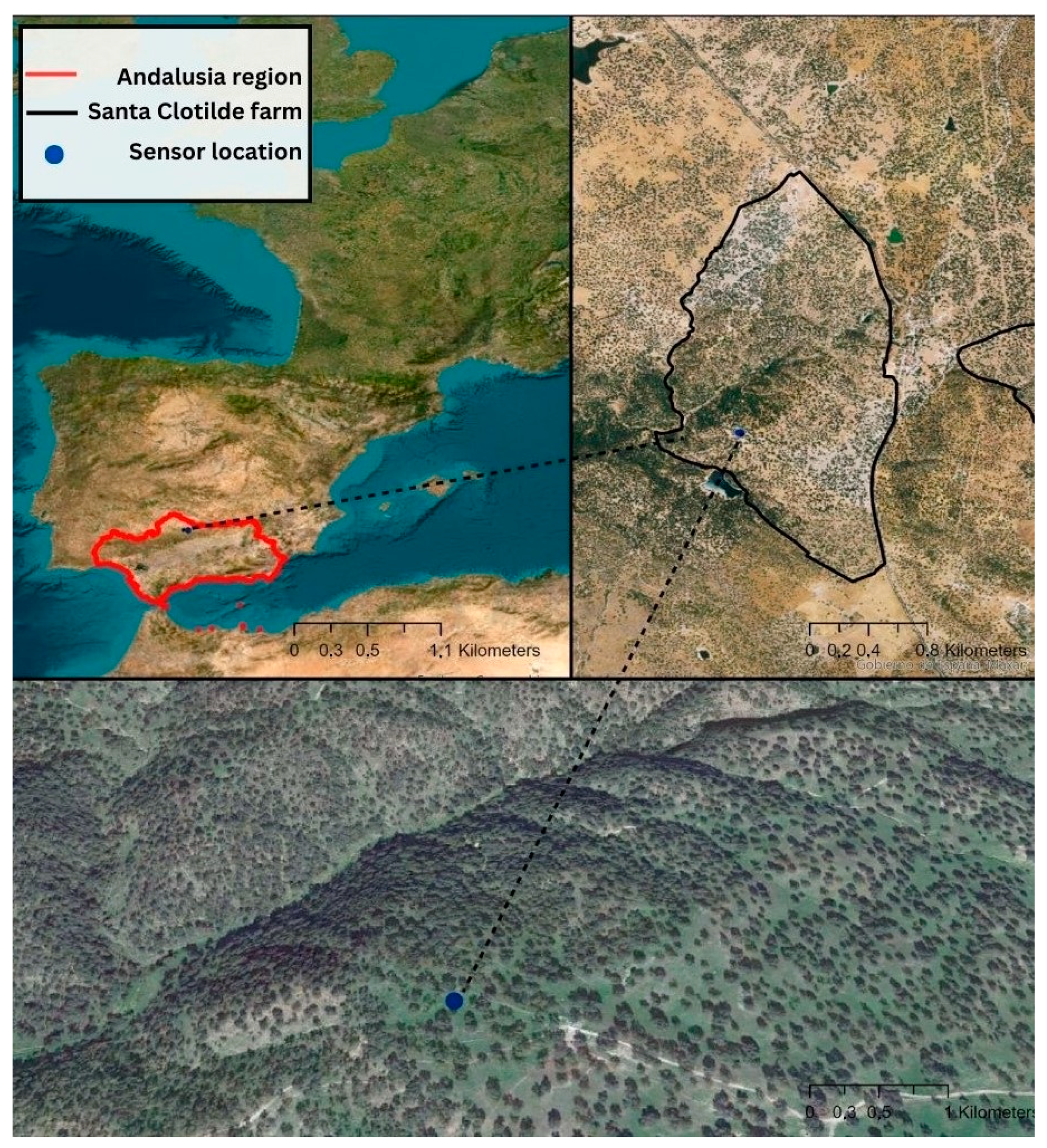
2.1. Study Area

The study was carried out at the Santa Clotilde commercial farm located in the north of the Córdoba province, Southern Spain (38.2° N; 4. 17° W, 700 m a.m.s.l.). The main activity of the Santa Clotilde farm is the extensive livestock production in the Dehesa agroforestry system (Figure 1); bovines and swine grazing there rotationally throughout the whole year. The soil texture is sandy loam according to the USDA (6.7% clay, 64% sand, 29.3% loam); due to rotational grazing, the first 30 cm of the soil profile holds 70% of the total carbon stock [53]. According to the Köppen–Geiger classification, the climate is Mediterranean, with an average annual rainfall of 878 mm, cold dry winter seasons, long summers, and a mean temperature of 25.4 °C [54]. For in-field monitoring of soil moisture dynamics, three TDR soil moisture sensors (Campbell Scientific CS655) were installed at different depths (5 cm, 15 cm, and 25 cm) in an open field, as shown in Supplementary Materials. Each sensor measured the soil moisture every hour. To compare the soil moisture dynamics with the satellite-derived SWI, which is representative within the top 20 cm of the soil, we decided to use the daily average value from the series of three sensors installed in the open field; the data are shown in Figure 2. The Campbell Scientific CS655 sensors used in this study are advanced TDR sensors, each consisting of two 30 cm long stainless steel waveguides connected to a printed circuit board. These sensors measure the soil moisture content with an accuracy of ±2.5% v/v for typical mineral soils. However, their accuracy and stability can be affected by the soil’s electrical conductivity and temperature, with the sensor output becoming unstable at electrical conductivity values greater than 20 dS/m. A temperature correction polynomial is provided to account for the sensor’s strong dependence on the soil temperature [55,56]. Precipitation data are obtained using the SM2RAIN-ASCAT satellite-based method. SM2RAIN-ASCAT is a global product obtained from the Advanced SCATterometer (ASCAT) satellite through the SM2RAIN algorithm developed by Brocca et al. [57]. The SM2RAIN algorithm allows for the calculation of rainfall using the inverse equation of water balance with in situ or satellite-based soil moisture data [58]. We also estimated the satellite-based Soil Water Index (SWI) at the study area. The SWI of the Copernicus Global Land Service [59] is acquired from measurements of near-surface soil moisture supplied by ASCAT by means of an algorithm that summarizes and exponentially weights past measurements according to the time length T, which ranges between 001 and 100 [60]. The T factor indicates how many past observations of surface soil moisture affect the current value of the SWI. Conceptually, a higher delay and an increasing smoothing signal detected at the soil surface from a higher T value is comparable to the effect of soil water infiltration. Thus, the SWI is a reliable proxy of soil moisture content at the 20 cm depth [57,61]. Specifically, this study has been selected with a value of the T-parameter equal to 20 days.

2.2. Soil Moisture Model

To estimate the soil moisture dynamics of the Mediterranean permanent grasslands, we modeled the soil moisture, using as water input the daily satellite rainfall data from ASCAT data [58]. The soil moisture dynamic model is conceptually based on the BEACH model [62], which divides the soil moisture reservoir in two layers: the top layer, whose depth is delimited by the root zone and whose water balance is determined by rainfall, evapotranspiration, runoff, and deep percolation; and the passive layer, where soil moisture is mainly driven by deep percolation. In this study, we simplify the model to only represent the top layer of 25 cm depth. Irrigation input is not considered because it is a rainfed grassland. The soil moisture model (SM25) calculates the volume of water stored in the soil (St; in mm), considering the stored volume from the previous day (S_t−1):

$$S_t=S_{t-1}+Rf-{ET}_{act}-Dp$$

(1)

where St is the daily soil moisture (mm); S_t−1 is the soil moisture of the antecedent day (mm); Rf is the net precipitation (mm); ET_act is the actual evapotranspiration (mm); and Dp is the deep percolation (mm).

To compute the Rf that reaches the soil surface, we apply the formula proposed by Morgan and Duzant [63]:

$$Rf=R-PI$$

(2)

where R is the total daily precipitation (mm) and PI is the plant interception (mm). To calculate PI, we apply the empirical equation proposed by Braden [64] as a function of the leaf area index (LAI), the canopy cover (CC) and the daily precipitation (R; in mm):

$$PI=aLAI\left(1-{\displaystyle \frac{1}{1+\frac{CCR}{aLAI}}}\right)$$

(3)

where PI is the daily plant interception (mm); a is an empirical coefficient that ranges between 0.3 (before senescence) and 0.6 (end of the senescence period) [65]; CC is the canopy cover; and LAI is the leaf area index. Similar to the DREAM model [66] and the SWAP model [67], the actual evapotranspiration (ETact) is calculated as a combination of the reference evapotranspiration (ET₀) from the vegetated fraction (CC) and the actual evaporation from the bare soil fraction (1 − CC):

$${ET}_{act}={ET}_{veg}CC+E_{soil}(1-CC)$$

(4)

where ET_veg is the actual daily evapotranspiration from the vegetated fraction (in millimeters) and E_soil is the actual daily evaporation of the bare soil fraction (in millimeters), shown in (5) and (6). Both ET_veg and E_soil depend on the degree of water availability in the soil. The degree of water availability is expressed by the actual soil moisture divided by the field-capacity soil moisture. This approach is based on the following assumptions (5) [68]:

If the soil moisture of the previous day is higher than the water stored in the soil at field capacity:

$${ET}_{veg}=ETo-PI$$

(5)

$$E_{soil}=ETo$$

(6)

therefore

$${ET}_{act}=\left(ETo-PI\right)CC+ETo(1-CC)$$

(7)

If the soil moisture of the previous day is lower than the water stored in the soil at field capacity (S_fc) and higher than at the wilting point (S_wp), ET_act is equal to the potential plant evapotranspiration (in mm) plus the actual soil daily evaporation of the bare soil fraction (in mm), then we have (8) and (9):

$${ET}_{veg}=\left(ETo-PI\right)\left({\displaystyle \frac{S_{t-1}-S_{wp}}{S_{fc}-S_{wp}}}\right)$$

(8)

$$E_{soil}=ETo\left({\displaystyle \frac{S_{t-1}-S_{wp}}{S_{fc}-S_{wp}}}\right)$$

(9)

Therefore (10):

$${ET}_{veg}=0 and {ET}_{soil}=0$$

(10)

Deep percolation Dp was simulated by applying the same BUDGET model method [69], given by (11):

$$Dp=d_s\tau ({\theta }_{sat}-{\theta }_{fc})\left({\displaystyle \frac{e^{\left(\theta {-\theta }_{fc}\right)}-1}{e^{{(\theta }_{sat}{-\theta }_{fc})}-1}}\right)$$

(11)

where d_s is the depth of the soil A-horizon (mm); θ is the soil moisture expressed as millimeters of water depth per millimeter of soil depth; θ_sat is the soil moisture at saturation; θ_fc is the soil moisture at field capacity; and τ is a drainage parameter, given by Equation (12):

$$0\le \tau ={0.0866}^{0.8063{log}_{10}\left(K_{sat}\right)}\le 1$$

(12)

where K_sat is the saturated hydraulic conductivity (mm d⁻¹).

2.3. Soil Moisture Model Calibration and Validation

For the soil moisture model calibration and validation, we used the observed daily soil moisture values from 17 March 2017 to 1 February 2021. Data from 17 March 2017 to 23 June 2019 were used for the model calibration and from 24 April 2019 to 12 February 2020 for the model validation. Model performance was evaluated using the Nash–Sutcliffe efficiency (NSE). NSE determines the relative magnitude of the residual variance compared with the observed data variance [70]. For the model calibration computation, we used the Non-dominated Sorting Genetic Algorithm (NSGA-II) and considered the following parameters: canopy cover (CC); saturated hydraulic conductivity in mm/day (Ksat); soil moisture ratio at wilting point in mm/mm (Swp); soil moisture ratio at field capacity in mm/mm (Sfc); and soil moisture ratio at wilting saturation in mm/mm (theta_sat). The NSGA-II was set to maximize the NSE.

2.4. NDVI Forecasting Models

The NDVI forecast model uses the available NDVI, temperature, and current soil moisture data to predict the NDVI values. We developed two NDVI forward-forecasting models using the two selected soil moisture products:

$$NDV{I}_{SWI}:NDVIt0+x~SWI+T20+NDVIt0$$

$$NDVI\_SM25:NDVIt0+x~SM\_25+T20+NDVIt0$$

where NDVI_t0+x is the forecasted NDVI at day t_0+x (7 or 30); SWI is the Soil Water index (SWI); and T20 is the cumulative mean temperature of the previous 20 days. T20 was selected instead of other cumulative day ranges based on it achieving the highest performance in terms of NSE values; NDVI_t0 is the observed NDVI value at present. The values were retrieved from the Copernicus Sentinel-2 using Google Earth Engine. Observed NDVI values were also used as a reference to compare the forecasted results. The observed NDVI corresponds to an area of 21 m radius, covering a grid of approximately 3 × 3 pixels with 10 m of spatial resolution, located in the hill–plateau of the Santa Clotilde farm in open grassland to avoiding the influence of trees; SM_25 is the simulated soil moisture at 25 cm soil depth. The grassland’s NDVI was predicted by applying the Random Forest machine learning algorithm [71]. This approach is composed of accumulation of singular decision trees (estimators) that allow an exceptional achievement of prediction accuracy [72]. Each tree’s predictions depend on randomly sampled values, and as we increase the number of trees in the forest, the overall predictive accuracy becomes more reliable. The effectiveness of a Random Forest depends on how strong the individual trees are and how much they correlate with each other. Unlike some other methods, Random Forests use a random selection of features for each tree, making them robust against noise. The algorithm internally monitors the error rates, the strength of predictions, and the correlations between trees. This information helps in assessing how well the model responds to an increasing number of features [71]. The training and testing of the NDVI forecast models were performed from 21 July 2015 to 30 December 2021, using 50% of the data for each one. Prediction performance was evaluated using the NSE and the mean bias error (MBE). MBE is used to estimate the bias between the predicted value and the observed value [73]. In comparison with the NSE, the MBE provides a view of how close the forecasts are to the measurements in absolute values, displayed respectively in (13) and (14).

$$NSE=1-{\displaystyle \frac{\sum _{t=1}^n{[q}_{obs}\left(t\right)-q_{sim}\left(t\right){]}^2}{\sum _{t=1}^n{[q}_{obs}\left(t\right)-{\overline{q}}_{obs}{]}^2}}$$

(13)

$$MBE={\displaystyle \frac{1}{n}}{\sum }_{t=1}^n(q_{obs}\left(t\right)-q_{sim}\left(t\right))$$

(14)

Moreover, we assessed the grassland vegetation response to droughts by filtering the NDVI dataset temporally. To calculate the vegetation response to environmental condition, we estimated the anomalies (Z-Score) [68] (15). Conceptually, these anomalies represent the intra-seasonal variations in the NDVI in response to fluctuations in the environmental conditions (e.g., drought conditions) [74].

$$Z-score={\displaystyle \frac{NDVIt-NDVImean,i}{NDVIstdi}}$$

(15)

where NDVI_t is the NDVI observed at time step t; NDVI_mean,i is the monthly mean of the NDVI daily values; and NDVI_stdi is the monthly standard deviation of the NDVI daily values. A positive or negative value of the Z-Score indicates a period wetter or drier than the average, respectively. This helps us identify exceptionally dry periods, which can have an important impact on grass production.

In order to evaluate the correlation between the anomalies (Z-Score) simulated by the NDVI models and the observed ones, we applied Pearson’s correlation (16):

$$r_{x,y}={\displaystyle \frac{{\sum }_{i=1}^n(x_i-\overline{x}\left)\right(y_i-\overline{y})}{\sqrt{{\sum }_{i=1}^n{\left(x_i-\overline{x}\right)}^2} \sqrt{{\sum }_{i=1}^n{\left(y_i-\overline{y}\right)}^2}}}$$

(16)

where r_x,y is the correlation coefficient; n is the length of the time series; i is the study period (in years); xi and yi are the NDVI anomalies, respectively; and x and y are the mean values of the NDVI. If the value of r_x,y is greater than zero, it is a positive relationship; if rx,y is a negative value, it is a negative relationship; if r_x,y is equal to zero, there is no relationship between the two variables [70]. In addition, a significance test was conducted, calculating the p-value with a significance level set at less than 0.05.

3. Results

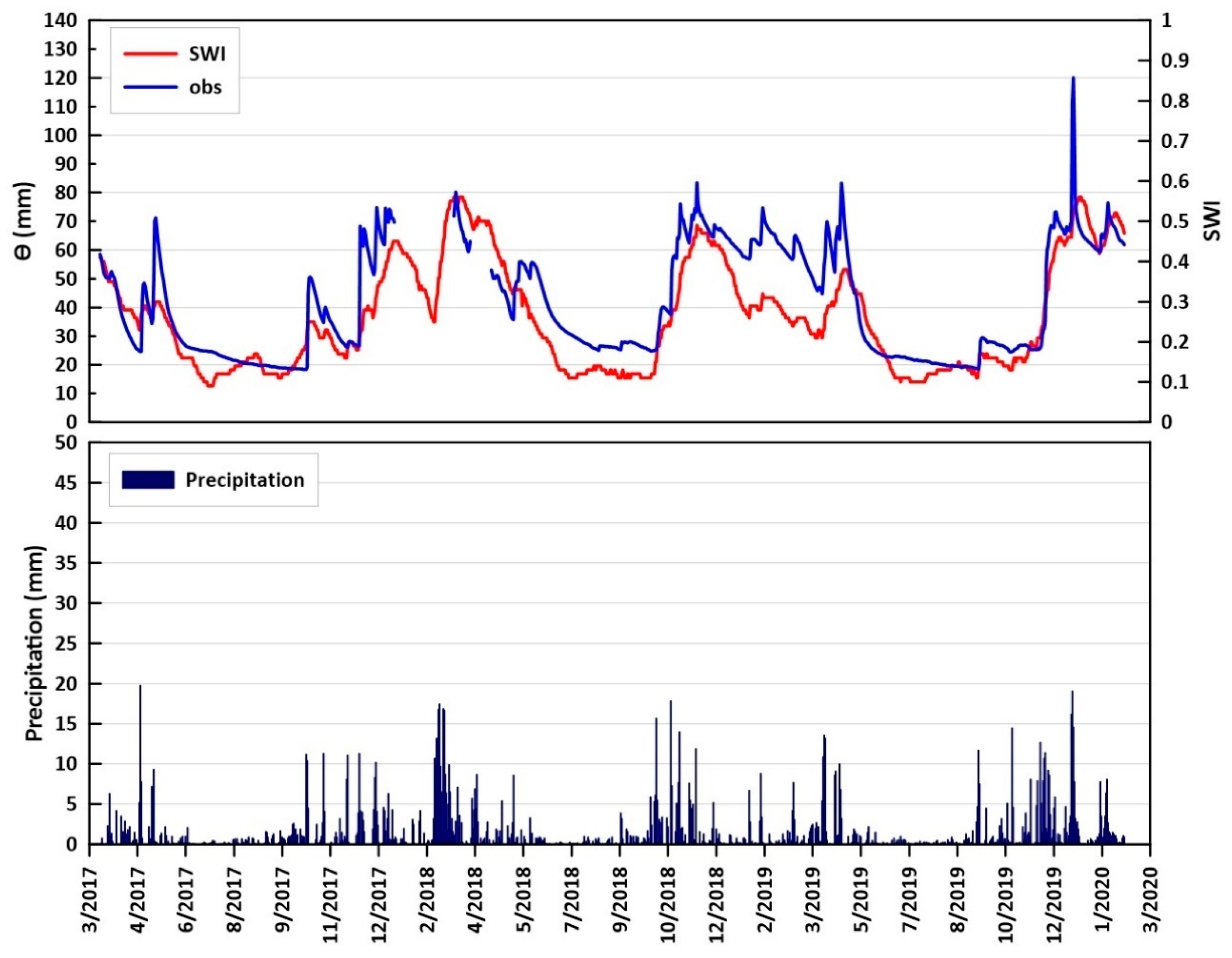
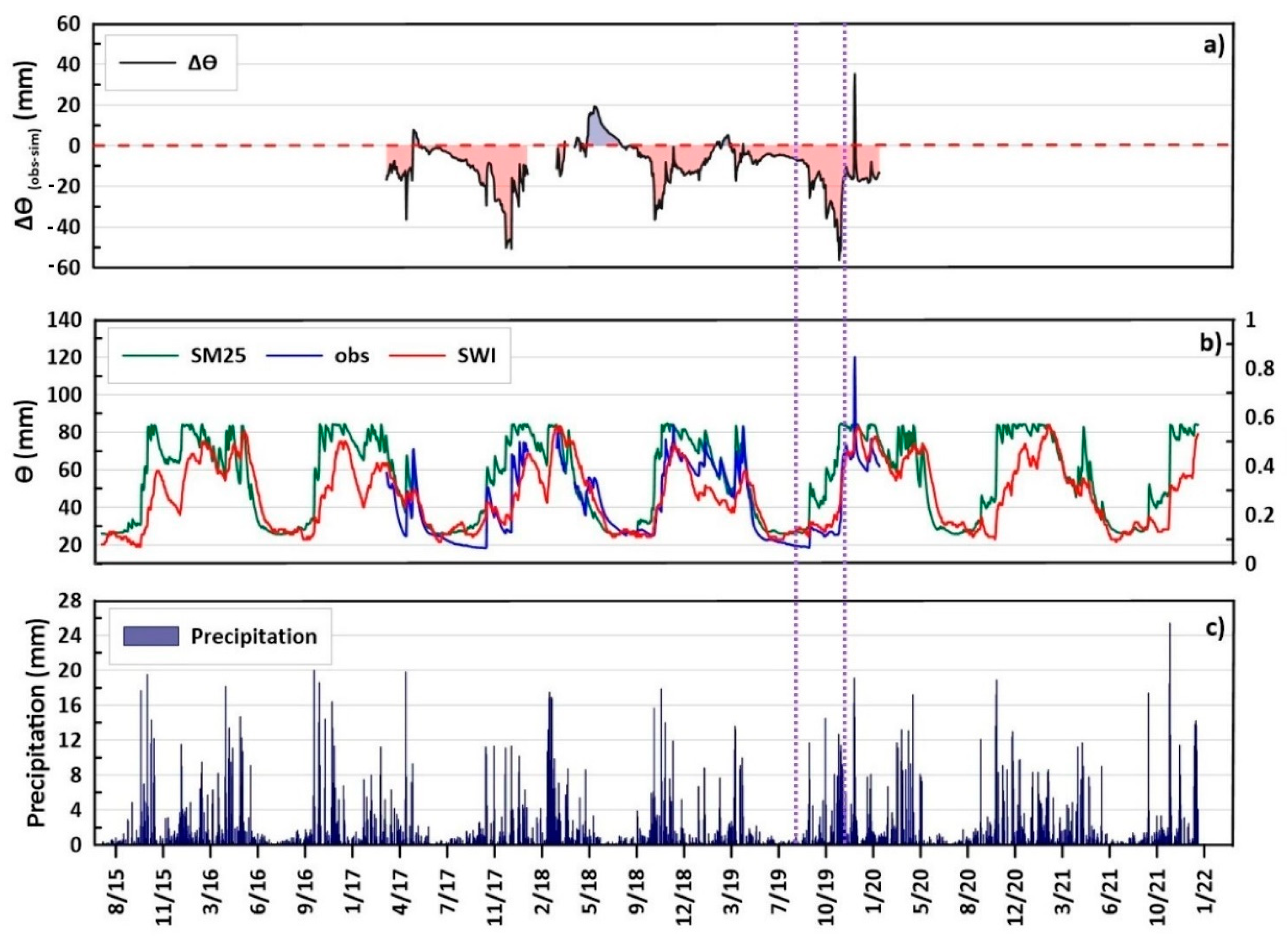
3.1. Soil Moisture Dynamics

The calibration and validation results of the soil moisture model yielded NSE values of 0.71 and 0.70, respectively (Supplementary Materials). This indicates that the model is able to satisfactorily simulate the observed soil moisture. In Figure 3, we compared the results of the soil moisture dynamics modeled over the study period. Figure 3a displays the difference between the ground-observed soil moisture and the simulated moisture values. The results show that the model generally overestimates the observed values. This can be explained by the fact that not all the precipitation events are reflected by sensors (e.g., see the dotted rectangle in Figure 3, where wet periods are not reflected in an increase in the observed soil moisture). It must be also noted that we are comparing values obtained at different spatial scales; the precipitation data and, hence, the model results are pixel values, while soil moisture observations are point values. Furthermore, sensors were deployed in open fields subject to rotational grazing; this dynamic scenario could potentially induce local modifications in the physical and hydraulic soil properties.

We observed differences between the two soil moisture products throughout the study period in how quickly they responded to precipitation. The SM25 reached higher values of soil moisture (in mm) more quickly than the SWI, as shown in Figure 3b. This may be due to a dissimilarity issue in the spatial scales between point (model) and pixel values (satellite observations) [75]. Differences between the two soil moisture products have been widely discussed. Deng et al. [76] analyzed and compared 670 soil moisture stations globally, highlighting that satellite products offer better correlation with observed data and more consistent performance compared with land surface models, which exhibit greater variability and a less accurate response to precipitation events. However, satellite products can present significant biases under specific climate and land cover conditions, while land surface models require improvements in their response to precipitation to enhance their reliability.

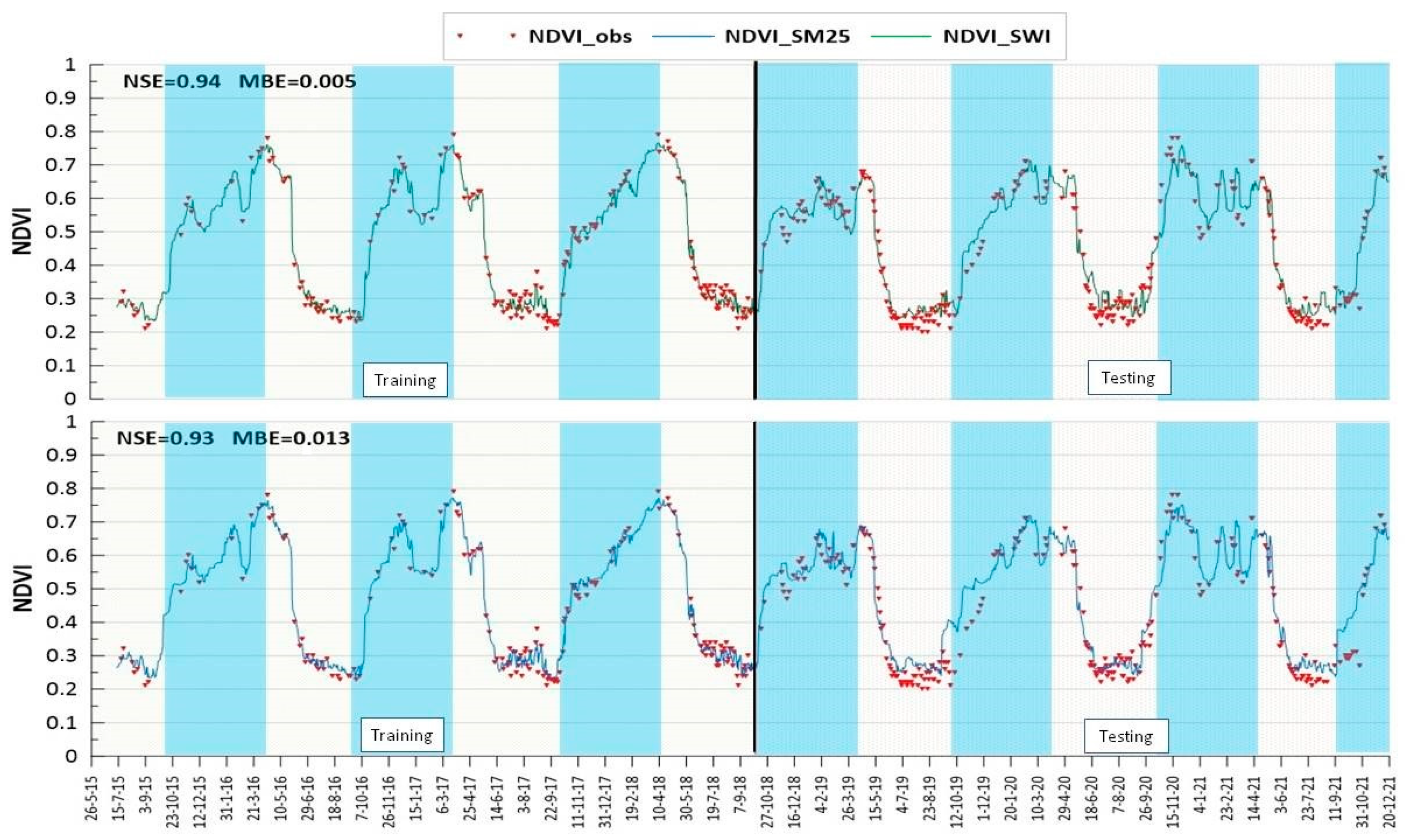
3.2. NDVI Forecasting Models Results

Figure 4 and Figure 5 show the results of the NDVI prediction at 7 and 30 days ahead, respectively. For both versions of the NDVI forecast model, the results are satisfactory. As expected, the 7-day lead time forecasts (NSE over 0.9 and MBE lower than 0.02) are better than the 30-day lead time forecasts (NSE over 0.80 and MBE lower than 0.02). The training and the testing model’s performances of NDVI forecasting model are displayed in

Table 1. Training and testing the NSE performance value for the different NDVI forecasting models.

Period	SWI7	SM257	SWI30	SM2530
Calibration	0.94	0.90	0.91	0.91
Validation	0.73	0.66	0.60	0.61

. From Figure 4 and Figure 5, we can break down the seasonal grassland dynamics into two main stages: the growing season (light blue area in Figure 4 and Figure 5), when NDVI values raise and reach the highest values, and the senescence season, when the NDVI decreases and reaches the lowest values. In the Mediterranean climate, the grassland growing season is characterized by a fluctuation in NDVI values during the productive season (harvest or grazing season) as a result of dry periods [77,78]; this underlines the relationship between the phonology dynamics and soil moisture dynamics [79]. The peak values of the NDVI obtained with both forecasting models at both 7- and 30-day lead times were between 0.50 and 0.80, which are in the order of magnitude of the observed values found in the literature for arid and semi-arid climates, which range between 0.53 and 0.78 [32]. These results not only demonstrate the significance of soil moisture as a driver of grassland dynamics in Mediterranean climates but also show the potential use of the two proposed NDVI forecasting models to predict seasonal variations in the NDVI. Regarding the intra-seasonal variations or anomalies (Z-score), Figure 6 and Figure 7 show that both NDVI_SM25 and NDVI_SWI for the 7-day lead time (r = 0.92, p-value < 0.05, for both models; see Table 1) perform better than for the 30-day lead time (NDVI_SWI30 r = 0.54, NDVI_SM2530 r = 0.60, p-value < 0.05;

Table 2. Pearson correlation (p-value < 0.05) between the observed NDVI anomalies and the forecasted anomalies at 7 and 30 days. The overall correlation takes into consideration the entire study period; the growing season (GS) correlation takes into consideration only the growing season of the study period; the 2017–2018 correlation takes into consideration the driest growing season of our study period.

Period	SWI7	SM257	SWI30	SM2530
Overall	0.92	0.92	0.54	0.60
GS	0.93	0.92	0.56	0.62
GS17-18	0.93	0.93	0.59	0.65

). We observe similar results comparing performances focusing only on the growing season. Indeed, both versions of the NDVI forecast models, NDVI_SWI7 and NDVI_SM257, showed satisfactory performances at the 7-day lead time, recording a high correlation with the observed anomalies (r = 0.93 and r = 0.92, respectively). Instead, the tNDVI forecast models at the 30-day lead time did not predict NDVI anomalies during the growing periods. However, the NDVI_SM2530 model predicts slightly better NDVI anomalies than the NDVI_SWI30 model (respectively, r = 0.56 and r = 0.62). Taking, as an example, the growing season of 2017–2018 with 454 mm of precipitation, and the season from 2018–2019, with 1796 mm (Figure 6 and Figure 7), we can observe how the models perform under particularly dry and wet weather conditions. Under these two conditions, both 7-day forecasting models predict anomalies satisfactorily (r = 0.93 for both models); in contrast, forecasting models at 30 days are weakly correlated to the observed anomalies (respectively, r = 0.59 for NDVI_SWI30 and r = 0.65 for NDVI_SM2530). This shows the limitation of using past and present data to forecast NDVI anomalies in the mid and long term. Future work should explore the use of mid- and long-range weather forecasting products to improve the performance of this type of NDVI forecasting model. In particular, NDVI_SM25 may benefit from using weather forecasting data to feed the soil moisture model and, thus, to obtain soil moisture forecasts of one or several months.

Prediction of NDVI anomalies gains particular importance in the context of agricultural insurance. In Spain, agricultural insurers, under the jurisdiction of the Spanish government, use the NDVI anomaly method to assess grassland yield loss caused by drought or extreme weather events, estimating remotely the production deficit with an NDVI-based indicator called the Guaranteed Vegetation Index [27]. It is calculated using data from the last 20 years and during the guaranteed period, which corresponds to the growing season, as the 10-day mean NDVI minus 0.5–1.5 times the 10-day standard deviation multiplied by an economical estimator. This model is based on past estimations; however, the use of NDVI forecasting models, such as the ones presented in this study, can let both farmers and insurers anticipate production deficits and, hence, compensations. However, it must be noted that their potential applicability is rather different. The SWI version, which uses satellite products, increases the potential of the scalability of its use from single pixel scales to larger areas comprising multiple pixels. The use of the soil moisture model version, combined with seasonal weather forecast data, could potentially increase the temporal scale and potentially obtain better performance for longer lead times than 7 days. While the results of the study are promising, we recognize that there were several limitations, such as there being only one observation point and the use of historical meteorological data. Considering the limited literature on the use of soil moisture products as NDVI predictors, we advise further investigation into other bioregions and at a larger scale. Moreover, the use of stationary weather prediction can be explored to extend the forecasting period to predict anomalies. Field NDVI assessment can be carried out to better fit the models and to assess discrepancies with satellite-based NDVI observations.

4. Discussion

The prediction of grassland dynamics and yield is a critical aspect of agricultural management, with various methods developed to enhance its accuracy and reliability. Traditional approaches have primarily relied on weather forecasting and management inputs, such as fertilizer application and temperature and precipitation data. However, the integration of soil moisture information has significantly improved these models, offering a more comprehensive understanding of the vegetation state. Remote sensing techniques, particularly the NDVI, have become essential tools in monitoring and predicting vegetation dynamics. The increasing application of machine learning algorithms has further revolutionized this field, providing powerful tools for developing forecasting and decision-making systems for land managers and stakeholders. This discussion explores the evolution and efficacy of these methods, emphasizing the advancements in remote sensing and machine learning that have enhanced the prediction of grassland growth dynamics. Various methods have been developed to predict grassland dynamics and yield using weather forecasting. McDonnell et al. [22] explored forecasts of grassland dynamics, incorporating management inputs like fertilizer application and weather inputs such as temperature and precipitation. Trnka et al. [23] improved grassland growth models by including soil moisture balance, which integrates weather, evapotranspiration, and plant-available water, enhancing the vegetation state information. Soil moisture can explain up to 60% of grassland yield variability and significantly improves productivity models [27].

Remote sensing techniques, especially the NDVI, are commonly used to monitor vegetation dynamics. The NDVI is a simple indicator of vegetation greenness and is widely used to estimate vegetation density and crop yields [28,29]. In Spain, the NDVI quantifies grassland yield losses and compensates for drought or extreme weather conditions during the growing season (October–June) [30]. Research has shown that the NDVI can be estimated from soil conditions, demonstrating a strong correlation in arid climates [31]. For instance, Chen et al. [29] found a good correlation between soil moisture and the NDVI in Australia, with the highest positive correlations when soil moisture precedes the NDVI by one month. In regions with dense tree cover, soil moisture and the NDVI are positively correlated over various temporal scales (0 to 5 months). In climates with prolonged dry seasons, such as in southern Spain, the NDVI correlates better with soil moisture than with precipitation [21,33]. Wang et al. [31] observed a stronger correlation in semi-arid regions than in humid areas of the USA. The NDVI has potential in supporting grazing and harvesting planning, especially in predicting water deficiencies and yield losses [35,36,37]. Autoregressive models, which forecast future NDVI values using past data, have shown high reliability in forestry land uses due to plant growth seasonality [38]. Iwasaki [39] attempted to predict the NDVI distribution using seasonal weather forecasts in an arid climate but found weak prediction efficiency. Parametric crop growth models have also been used to forecast the NDVI but have shown low accuracy compared with machine learning-based methods [41].

Machine learning algorithms, enabled by advancements in remote sensing and agricultural digitalization, offer robust forecasting tools for land managers, farmers, and agro-forestry stakeholders [42,43,44]. However, predicting vegetation development remains challenging due to multiple ecosystem processes that affect vegetation dynamics [52,53]. Process-based models struggle to accurately predict vegetation dynamics because they cannot adequately interrelate these ecosystem processes [53]. Consequently, the use of machine learning, with its high performance and broad applicability, is rapidly increasing worldwide [54]. Approaches such as artificial neural networks, support vector regression, Random Forests, and regression trees are widely used to predict vegetation dynamics. These methods do not rely on relationships between predictors and the predictive variable, unlike traditional models such as linear regression, which assume a Gaussian distribution for input variables [56].

Roy [50] found that the Random Forest algorithm performed best in forecasting the average large-area NDVI in Bangladesh. Wang et al. [51] and Yin et al. [52] also demonstrated the efficacy of the Random Forest method in predicting pasture dynamics. On the Loess Plateau, the model forecasted a westward decrease in the aboveground biomass (AGB), identifying the NDVI as a key factor. On the Tibetan Plateau, the Random Forest model accurately predicted pasture height, considering seven influential variables. Both studies highlight the effectiveness of this machine learning model in understanding pasture dynamics across diverse environmental conditions. The integration of NDVI forecasts based on soil moisture represents a significant advancement in agricultural and environmental management, particularly for Mediterranean landscapes characterized by prolonged dry seasons and irregular precipitation. The results of our study clearly indicate that soil moisture, whether derived from in situ sensors or satellite observations, plays a crucial role in determining the growth dynamics of permanent grasslands in these regions. This finding not only confirms what has been suggested by previous studies but also extends the applicability of NDVI forecasts to contexts characterized by adverse and variable climatic conditions. The ability of the models to predict grassland growth dynamics with a lead time of 7 and 30 days not only provides a useful predictive tool for agricultural planning but also demonstrates the validity of integrating satellite data into environmental modeling. This is particularly relevant for Mediterranean regions, where access to in situ measurements may be limited, and the spatial variability in soil moisture can significantly impact vegetation production. However, this study presents some limitations that require further investigation. Firstly, the spatial scale of the soil moisture measurements is limited, which could reduce the generalizability of the results to larger or different areas. The accuracy of the models may vary in contexts where the distribution of soil moisture is more heterogeneous or where other environmental factors, such as soil type or varying vegetation cover, have a greater influence on vegetation dynamics. Moreover, while the developed models show high reliability in predicting the NDVI, the relationship between the NDVI and biomass production remains to be further explored. This aspect is fundamental for translating NDVI forecasts into more precise estimates of agricultural productivity, which could be used to develop more effective and targeted agricultural and forestry management policies. Expanding this approach to a larger scale and integrating additional environmental variables could contribute to improving the accuracy and practical utility of the forecasts, offering a valuable tool not only for farmers but also for insurance agencies and policymakers. Although our study confirms the potential of NDVI models based on machine learning and soil moisture data, the challenge remains to validate these results on broader spatial scales and in different environmental contexts. Further research could focus on integrating this approach with biomass growth models in order to develop more comprehensive and useful forecasting tools for the sustainable management of agroforestry resources in Mediterranean landscapes and beyond.

5. Conclusions

In this study, we present two NDVI forecasting models based on the use of machine learning and past and present weather and soil moisture data as predictors. One model, NDVI_SM25, uses simulated soil moisture values, and the other, NDVI_SWI, uses satellite-based Soil Water Index (SWI) values. The performance of both models was evaluated in a Mediterranean permanent grassland in southern Spain by comparing forecasted and observed NDVI daily values. Results show high reliability of the models at 7 and 30-day forecast lead times in predicting seasonal NDVI dynamics and demonstrate the significance of soil moisture dynamics as a driver of grassland phenology in dry climates. In the case of intra-seasonal variations or anomalies, the NDVI is significantly better predicted by both models at a 7-day lead time than at a 30-day lead time. These results show the potential of using NDVI forecasting models based on soil moisture information and machine learning to help both farmers and insurers anticipate production deficits and apply mitigation measures.

References

1. Bugalho, M.N.; Caldeira, M.C.; Pereira, J.S.; Aronson, J.; Pausas, J.G. Mediterranean Cork Oak Savannas Require Human Use to Sustain Biodiversity and Ecosystem Services. Front. Ecol. Environ. 2011, 9, 278–286. [Google Scholar] [CrossRef] [PubMed]
2. Pulido, F.J.; Díaz, M.; Hidalgo de Trucios, S.J. Size Structure and Regeneration of Spanish Holm Oak Quercus Ilex Forests and Dehesas: Effects of Agroforestry Use on Their Long-Term Sustainability. For. Ecol. Manag. 2001, 146, 1–13. [Google Scholar] [CrossRef]
3. Schils, R.L.M.; Bufe, C.; Rhymer, C.M.; Francksen, R.M.; Klaus, V.H.; Abdalla, M.; Milazzo, F.; Lellei-Kovács, E.; Berge, H.T.; Bertora, C.; et al. Permanent Grasslands in Europe: Land Use Change and Intensification Decrease Their Multifunctionality. Agric. Ecosyst. Environ. 2022, 330, 107891. [Google Scholar] [CrossRef]
4. Shujun, G. The Meteorological Disaster Risk Assessment Based on the Diffusion Mechanism. J. Risk Anal. Crisis Response 2012, 2, 124. [Google Scholar]
5. Zhao, A.; Yu, Q.; Feng, L.; Zhang, A.; Pei, T. Evaluating the Cumulative and Time-Lag Effects of Drought on Grassland Vegetation: A Case Study in the Chinese Loess Plateau. J. Environ. Manag. 2020, 261, 110214. [Google Scholar] [CrossRef]
6. Chang, S.; Chen, H.; Wu, B.; Nasanbat, E.; Yan, N.; Davdai, B. A Practical Satellite-Derived Vegetation Drought Index for Arid and Semi-Arid Grassland Drought Monitoring. Remote Sens. 2021, 13, 414. [Google Scholar] [CrossRef]
7. Warter, M.M.; Singer, M.B.; Cuthbert, M.O.; Roberts, D.; Caylor, K.K.; Sabathier, R.; Stella, J. Drought Onset and Propagation into Soil Moisture and Grassland Vegetation Responses during the 2012–2019 Major Drought in Southern California. Hydrol. Earth Syst. Sci. 2021, 25, 3713–3729. [Google Scholar] [CrossRef]
8. Kowalski, K.; Okujeni, A.; Hostert, P. A Generalized Framework for Drought Monitoring across Central European Grassland Gradients with Sentinel-2 Time Series. Remote Sens. Environ. 2023, 286, 113449. [Google Scholar] [CrossRef]
9. Oukaddour, K.; Le Page, M.; Fakir, Y. Toward a Redefinition of Agricultural Drought Periods—A Case Study in a Mediterranean Semi-Arid Region. Remote Sens. 2024, 16, 83. [Google Scholar] [CrossRef]
10. Essa, Y.H.; Hirschi, M.; Thiery, W.; El-Kenawy, A.M.; Yang, C. Drought Characteristics in Mediterranean under Future Climate Change. Npj Clim. Atmos. Sci. 2023, 6, 133. [Google Scholar] [CrossRef]
11. Almeida-Ñauñay, A.F.; Villeta, M.; Quemada, M.; Tarquis, A.M. Assessment of Drought Indexes on Different Time Scales: A Case in Semiarid Mediterranean Grasslands. Remote Sens. 2022, 14, 565. [Google Scholar] [CrossRef]
12. He, X.; Estes, L.; Konar, M.; Tian, D.; Anghileri, D.; Baylis, K.; Evans, T.P.; Sheffield, J. Integrated Approaches to Understanding and Reducing Drought Impact on Food Security across Scales. Curr. Opin. Environ. Sustain. 2019, 40, 43–54. [Google Scholar] [CrossRef]
13. Rasheed, M.W.; Tang, J.; Sarwar, A.; Shah, S.; Saddique, N.; Khan, M.U.; Imran Khan, M.; Nawaz, S.; Shamshiri, R.R.; Aziz, M.; et al. Soil Moisture Measuring Techniques and Factors Affecting the Moisture Dynamics: A Comprehensive Review. Sustainability 2022, 14, 11538. [Google Scholar] [CrossRef]
14. Peng, J.; Loew, A. Recent Advances in Soil Moisture Estimation from Remote Sensing. Water 2017, 9, 530. [Google Scholar] [CrossRef]
15. Chen, Q.; Miao, F.; Wang, H.; Xu, Z.-X.; Tang, Z.; Yang, L.; Qi, S. Downscaling of Satellite Remote Sensing Soil Moisture Products Over the Tibetan Plateau Based on the Random Forest Algorithm: Preliminary Results. Earth Space Sci. 2020, 7, e2020EA001265. [Google Scholar] [CrossRef]
16. Rahimzadeh-Bajgiran, P.; Berg, A.A.; Champagne, C.; Omasa, K. Estimation of Soil Moisture Using Optical/Thermal Infrared Remote Sensing in the Canadian Prairies. ISPRS J. Photogramm. Remote Sens. 2013, 83, 94–103. [Google Scholar] [CrossRef]
17. Zhang, J.; Zhou, Z.; Yao, F.; Yang, L.; Hao, C. Validating the Modified Perpendicular Drought Index in the North China Region Using In Situ Soil Moisture Measurement. IEEE Geosci. Remote Sens. Lett. 2015, 12, 542–546. [Google Scholar] [CrossRef]
18. Efremova, N.; Seddik, M.E.A.; Erten, E. Soil Moisture Estimation Using Sentinel-1/-2 Imagery Coupled with CycleGAN for Time-Series Gap Filing. IEEE Trans. Geosci. Remote Sens. 2022, 60, 4705111. [Google Scholar] [CrossRef]
19. Yu, W.; Li, J.; Liu, Q.; Zhao, J.; Dong, Y.; Wang, C.; Lin, S.; Zhu, X.; Zhang, H. Spatial–Temporal Prediction of Vegetation Index With Deep Recurrent Neural Networks. IEEE Geosci. Remote Sens. Lett. 2022, 19, 1–5. [Google Scholar] [CrossRef]
20. Geng, X.; Li, H.; Yao, Z.; Chen, X.; Yang, Z.; Li, S.; Wu, L.; Cui, Y. Potential of ANN for Prolonging Remote Sensing-Based Soil Moisture Products for Long-Term Time Series Analysis. IEEE Geosci. Remote Sens. Lett. 2022, 19, 1–5. [Google Scholar] [CrossRef]
21. Tong, C.; Wang, H.; Magagi, R.; Goïta, K.; Wang, K. Spatial Gap-Filling of SMAP Soil Moisture Pixels Over Tibetan Plateau via Machine Learning Versus Geostatistics. IEEE J. Sel. Top. Appl. Earth Obs. Remote Sens. 2021, 14, 9899–9912. [Google Scholar] [CrossRef]
22. McDonnell, J.; Brophy, C.; Ruelle, E.; Shalloo, L.; Lambkin, K.; Hennessy, D. Weather Forecasts to Enhance an Irish Grass Growth Model. Eur. J. Agron. 2019, 105, 168–175. [Google Scholar] [CrossRef]
23. Trnka, M.; Eitzinger, J.; Gruszczynski, G.; Buchgraber, K.; Resch, R.; Schaumberger, A. A Simple Statistical Model for Predicting Herbage Production from Permanent Grassland. Grass Forage Sci. 2006, 61, 253–271. [Google Scholar] [CrossRef]
24. Krueger, E.S.; Ochsner, T.E.; Levi, M.R.; Basara, J.B.; Snitker, G.J.; Wyatt, B.M. Grassland Productivity Estimates Informed by Soil Moisture Measurements: Statistical and Mechanistic Approaches. Agron. J. 2021, 113, 3498–3517. [Google Scholar] [CrossRef]
25. Wang, J.; Rich, P.M.; Price, K.P.; Kettle, W.D. Relations between NDVI, Grassland Production, and Crop Yield in the Central Great Plains. Geocarto Int. 2005, 20, 5–11. [Google Scholar] [CrossRef]
26. Xue, J.; Su, B. Significant Remote Sensing Vegetation Indices: A Review of Developments and Applications. J. Sens. 2017, 2017, e1353691. [Google Scholar] [CrossRef]
27. BOLETÍN OFICIAL DEL ESTADO. BOE.Es-BOE-A-2022-6738 Orden APA/355/2022; de 18 de Abril; 2022; Available online: https://www.boe.es/boe/dias/2022/04/26/pdfs/BOE-A-2022-6738.pdf (accessed on 12 August 2024).
28. Han, Y.; Wang, Y.; Zhao, Y. Estimating Soil Moisture Conditions of the Greater Changbai Mountains by Land Surface Temperature and NDVI. IEEE Trans. Geosci. Remote Sens. 2010, 48, 2509–2515. [Google Scholar] [CrossRef]
29. Chen, T.; de Jeu, R.A.M.; Liu, Y.Y.; van der Werf, G.R.; Dolman, A.J. Using Satellite Based Soil Moisture to Quantify the Water Driven Variability in NDVI: A Case Study over Mainland Australia. Remote Sens. Environ. 2014, 140, 330–338. [Google Scholar] [CrossRef]
30. García-Gamero, V.; Peña, A.; Laguna, A.M.; Giráldez, J.V.; Vanwalleghem, T. Factors Controlling the Asymmetry of Soil Moisture and Vegetation Dynamics in a Hilly Mediterranean Catchment. J. Hydrol. 2021, 598, 126207. [Google Scholar] [CrossRef]
31. Wang, X.; Xie, H.; Guan, H.; Zhou, X. Different Responses of MODIS-Derived NDVI to Root-Zone Soil Moisture in Semi-Arid and Humid Regions. J. Hydrol. 2007, 340, 12–24. [Google Scholar] [CrossRef]
32. Insua, J.R.; Utsumi, S.A.; Basso, B. Estimation of Spatial and Temporal Variability of Pasture Growth and Digestibility in Grazing Rotations Coupling Unmanned Aerial Vehicle (UAV) with Crop Simulation Models. PLoS ONE 2019, 14, e0212773. [Google Scholar] [CrossRef]
33. Bounouh, O.; Tarquis, A.M.; Farah, I.R. Novel Method for Combining NDVI Time Series Forecasting Models. In Proceedings of the IGARSS 2022-2022 IEEE International Geoscience and Remote Sensing Symposium, Kuala Lumpur, Malaysia, 17–22 July 2022; pp. 2355–2357. [Google Scholar]
34. Iwasaki, H. NDVI Prediction over Mongolian Grassland Using GSMaP Precipitation Data and JRA-25/JCDAS Temperature Data. J. Arid. Environ. 2009, 73, 557–562. [Google Scholar] [CrossRef]
35. Ahmad, R.; Yang, B.; Ettlin, G.; Berger, A.; Rodríguez-Bocca, P. A Machine-Learning Based ConvLSTM Architecture for NDVI Forecasting. Int. Trans. Oper. Res. 2020, 30, 2025–2048. [Google Scholar] [CrossRef]
36. Berger, A.; Ettlin, G.; Quincke, C.; Rodríguez-Bocca, P. Predicting the Normalized Difference Vegetation Index (NDVI) by Training a Crop Growth Model with Historical Data. Comput. Electron. Agric. 2019, 161, 305–311. [Google Scholar] [CrossRef]
37. Casanova, J.J.; O’Shaughnessy, S.A.; Evett, S.R.; Rush, C.M. Development of a Wireless Computer Vision Instrument to Detect Biotic Stress in Wheat. Sensors 2014, 14, 17753–17769. [Google Scholar] [CrossRef]
38. Hadria, R.; Benabdelouahab, T.; Elmansouri, L.; Gadouali, F.; Ouatiki, H.; Lebrini, Y.; Boudhar, A.; Salhi, A.; Lionboui, H. Derivation of Air Temperature of Agricultural Areas of Morocco from Remotely Land Surface Temperature Based on the Updated Köppen-Geiger Climate Classification. Model. Earth Syst. Environ. 2019, 5, 1883–1892. [Google Scholar] [CrossRef]
39. Htitiou, A.; Boudhar, A.; Lebrini, Y.; Hadria, R.; Lionboui, H.; Benabdelouahab, T. A Comparative Analysis of Different Phenological Information Retrieved from Sentinel-2 Time Series Images to Improve Crop Classification: A Machine Learning Approach. Geocarto Int. 2022, 37, 1426–1449. [Google Scholar] [CrossRef]
40. Rehman, T.U.; Mahmud, M.d.S.; Chang, Y.K.; Jin, J.; Shin, J. Current and Future Applications of Statistical Machine Learning Algorithms for Agricultural Machine Vision Systems. Comput. Electron. Agric. 2019, 156, 585–605. [Google Scholar] [CrossRef]
41. Pereira, L.A.M.; Nakamura, R.Y.M.; de Souza, G.F.S.; Martins, D.; Papa, J.P. Aquatic Weed Automatic Classification Using Machine Learning Techniques. Comput. Electron. Agric. 2012, 87, 56–63. [Google Scholar] [CrossRef]
42. Haghverdi, A.; Leib, B.G.; Washington-Allen, R.A.; Ayers, P.D.; Buschermohle, M.J. Perspectives on Delineating Management Zones for Variable Rate Irrigation. Comput. Electron. Agric. 2015, 117, 154–167. [Google Scholar] [CrossRef]
43. Boydell, B.; McBratney, A.B. Identifying Potential Within-Field Management Zones from Cotton-Yield Estimates. Precis. Agric. 2002, 3, 9–23. [Google Scholar] [CrossRef]
44. Liu, S.; Cossell, S.; Tang, J.; Dunn, G.; Whitty, M. A Computer Vision System for Early Stage Grape Yield Estimation Based on Shoot Detection. Comput. Electron. Agric. 2017, 137, 88–101. [Google Scholar] [CrossRef]
45. Park, J.Y.; Ale, S.; Teague, W.R.; Dowhower, S.L. Simulating Hydrologic Responses to Alternate Grazing Management Practices at the Ranch and Watershed Scales. J. Soil Water Conserv. 2017, 72, 102–121. [Google Scholar] [CrossRef]
46. Xia, J.; Yuan, W.; Lienert, S.; Joos, F.; Ciais, P.; Viovy, N.; Wang, Y.; Wang, X.; Zhang, H.; Chen, Y.; et al. Global Patterns in Net Primary Production Allocation Regulated by Environmental Conditions and Forest Stand Age: A Model-Data Comparison. J. Geophys. Res. Biogeosci. 2019, 124, 2039–2059. [Google Scholar] [CrossRef]
47. Dokic, K.; Blaskovic, L.; Mandusic, D. From Machine Learning to Deep Learning in Agriculture—The Quantitative Review of Trends. IOP Conf. Ser. Earth Environ. Sci. 2020, 614, 012138. [Google Scholar] [CrossRef]
48. Xie, S.; Du, J.; Zhou, X.; Zhang, X.; Feng, X.; Zheng, W.; Li, Z.; Xu, C.-Y. A Progressive Segmented Optimization Algorithm for Calibrating Time-Variant Parameters of the Snowmelt Runoff Model (SRM). J. Hydrol. 2018, 566, 470–483. [Google Scholar] [CrossRef]
49. Li, X.; Yuan, W.; Dong, W. A Machine Learning Method for Predicting Vegetation Indices in China. Remote Sens. 2021, 13, 1147. [Google Scholar] [CrossRef]
50. Roy, B. Optimum Machine Learning Algorithm Selection for Forecasting Vegetation Indices: MODIS NDVI & EVI. Remote Sens. Appl. Soc. Environ. 2021, 23, 100582. [Google Scholar] [CrossRef]
51. Wang, Y.; Wu, G.; Deng, L.; Tang, Z.; Wang, K.; Sun, W.; Shangguan, Z. Prediction of Aboveground Grassland Biomass on the Loess Plateau, China, Using a Random Forest Algorithm. Sci. Rep. 2017, 7, 6940. [Google Scholar] [CrossRef] [PubMed]
52. Yin, J.; Feng, Q.; Liang, T.; Meng, B.; Yang, S.; Gao, J.; Ge, J.; Hou, M.; Liu, J.; Wang, W.; et al. Estimation of Grassland Height Based on the Random Forest Algorithm and Remote Sensing in the Tibetan Plateau. IEEE J. Sel. Top. Appl. Earth Obs. Remote Sens. 2020, 13, 178–186. [Google Scholar] [CrossRef]
53. Catorci, A.; Lulli, R.; Malatesta, L.; Tavoloni, M.; Tardella, F.M. How the Interplay between Management and Interannual Climatic Variability Influences the NDVI Variation in a Sub-Mediterranean Pastoral System: Insight into Sustainable Grassland Use under Climate Change. Agric. Ecosyst. Environ. 2021, 314, 107372. [Google Scholar] [CrossRef]
54. Peel, M.C.; Finlayson, B.L.; McMahon, T.A. Updated World Map of the Köppen-Geiger Climate Classification. Hydrol. Earth Syst. Sci. 2007, 11, 1633–1644. [Google Scholar] [CrossRef]
55. Campbell Scientific Operational Specifications. Available online: https://help.campbellsci.com/cs650-cs655/cs650-cs655/specifications/operational-specifications.htm?Highlight=Accurancy (accessed on 28 July 2024).
56. Walker, J.P.; Willgoose, G.R.; Kalma, J.D. In Situ Measurement of Soil Moisture: A Comparison of Techniques. J. Hydrol. 2004, 293, 85–99. [Google Scholar] [CrossRef]
57. Brocca, L.; Hasenauer, S.; Lacava, T.; Melone, F.; Moramarco, T.; Wagner, W.; Dorigo, W.; Matgen, P.; Martínez-Fernández, J.; Llorens, P.; et al. Soil Moisture Estimation through ASCAT and AMSR-E Sensors: An Intercomparison and Validation Study across Europe. Remote Sens. Environ. 2011, 115, 3390–3408. [Google Scholar] [CrossRef]
58. Brocca, L.; Filippucci, P.; Hahn, S.; Ciabatta, L.; Massari, C.; Camici, S.; Schüller, L.; Bojkov, B.; Wagner, W. SM2RAIN–ASCAT (2007–2018): Global Daily Satellite Rainfall Data from ASCAT Soil Moisture Observations. Earth Syst. Sci. Data 2019, 11, 1583–1601. [Google Scholar] [CrossRef]
59. Bauer-Marschallinger, B.; Paulik, C.; Hochstöger, S.; Mistelbauer, T.; Modanesi, S.; Ciabatta, L.; Massari, C.; Brocca, L.; Wagner, W. Soil Moisture from Fusion of Scatterometer and SAR: Closing the Scale Gap with Temporal Filtering. Remote Sens. 2018, 1019, 1030. [Google Scholar] [CrossRef]
60. Wagner, W.; Lemoine, G.; Borgeaud, M.; Rott, H. A Study of Vegetation Cover Effects on ERS Scatterometer Data. IEEE Trans. Geosci. Remote Sens. 1999, 37, 938–948. [Google Scholar] [CrossRef]
61. Paulik, C.; Dorigo, W.; Wagner, W.; Kidd, R. Validation of the ASCAT Soil Water Index Using in Situ Data from the International Soil Moisture Network. Int. J. Appl. Earth Obs. Geoinf. 2014, 30, 1–8. [Google Scholar] [CrossRef]
62. Sheikh, V.; Visser, S.; Stroosnijder, L. A Simple Model to Predict Soil Moisture: Bridging Event and Continuous Hydrological (BEACH) Modelling. Environ. Model. Softw. 2009, 24, 542–556. [Google Scholar] [CrossRef]
63. Morgan, R.P.C.; Duzant, J.H. Modified MMF (Morgan–Morgan–Finney) Model for Evaluating Effects of Crops and Vegetation Cover on Soil Erosion. Earth Surf. Process. Landf. 2008, 33, 90–106. [Google Scholar] [CrossRef]
64. Braden, H.; Deutscher, W. The Model AMBETI; Berichte des Deutschen Wetterdienstes: Offenbach am Main, Germany, 1995.
65. Arnold, J.G.; Moriasi, D.N.; Gassman, P.W.; Abbaspour, K.C.; White, M.J.; Srinivasan, R.; Santhi, C.; Harmel, R.D.; Van Griensven, A.; Van Liew, M.W.; et al. SWAT: Model Use, Calibration, and Validation. Trans. ASABE 2012, 55, 1491–1508. [Google Scholar] [CrossRef]
66. Manfreda, S.; Fiorentino, M.; Iacobellis, V. DREAM: A Distributed Model for Runoff, Evapotranspiration, and Antecedent Soil Moisture Simulation. Adv. Geosci. 2005, 2, 31–39. [Google Scholar] [CrossRef]
67. Kroese, D.P.; Brereton, T.; Taimre, T.; Botev, Z.I. Why the Monte Carlo Method Is so Important Today. WIREs Comput. Stat. 2014, 6, 386–392. [Google Scholar] [CrossRef]
68. Singh, V.P. Computer Models of Watershed Hydrology; Water Resources Publications: Littleton, CO, USA, 1995. [Google Scholar]
69. Raes, D.; Geerts, S.; Kipkorir, E.; Wellens, J.; Sahli, A. Simulation of Yield Decline as a Result of Water Stress with a Robust Soil Water Balance Model. Agric. Water Manag. 2006, 81, 335–357. [Google Scholar] [CrossRef]
70. Nash, J.E.; Sutcliffe, J.V. River Flow Forecasting through Conceptual Models Part I—A Discussion of Principles. J. Hydrol. 1970, 10, 282–290. [Google Scholar] [CrossRef]
71. Breiman, L. Random Forests. Mach. Learn. 2001, 45, 5–32. [Google Scholar] [CrossRef]
72. Zaimes, G.N.; Gounaridis, D.; Symenonakis, E. Assessing the Impact of Dams on Riparian and Deltaic Vegetation Using Remotely-Sensed Vegetation Indices and Random Forests Modelling. Ecol. Indic. 2019, 103, 630–641. [Google Scholar] [CrossRef]
73. Li, Z.; Rahman, S.M.; Vega, R.; Dong, B. A Hierarchical Approach Using Machine Learning Methods in Solar Photovoltaic Energy Production Forecasting. Energies 2016, 9, 55. [Google Scholar] [CrossRef]
74. Kogan, F.; Gitelson, A.; Zakarin, E.; Spivak, L.; Lebed, L. AVHRR-Based Spectral Vegetation Index for Quantitative Assessment of Vegetation State and Productivity. Photogramm. Eng. Remote Sens. 2003, 69, 899–906. [Google Scholar] [CrossRef]
75. Gruber, A.; Dorigo, W.A.; Zwieback, S.; Xaver, A.; Wagner, W. Characterizing Coarse-Scale Representativeness of in Situ Soil Moisture Measurements from the International Soil Moisture Network. Vadose Zone J. 2013, 12, vzj2012.0170. [Google Scholar] [CrossRef]
76. Deng, Y.; Wang, S.; Bai, X.; Wu, L.; Cao, Y.; Li, H.; Wang, M.; Li, C.; Yang, Y.; Hu, Z.; et al. Comparison of Soil Moisture Products from Microwave Remote Sensing, Land Model, and Reanalysis Using Global Ground Observations. Hydrol. Process. 2020, 34, 836–851. [Google Scholar] [CrossRef]
77. Chelli, S.; Canullo, R.; Campetella, G.; Schmitt, A.O.; Bartha, S.; Cervellini, M.; Wellstein, C. The Response of Sub-Mediterranean Grasslands to Rainfall Variation Is Influenced by Early Season Precipitation. Appl. Veg. Sci. 2016, 19, 611–619. [Google Scholar] [CrossRef]
78. Zavaleta, E.S.; Shaw, M.R.; Chiariello, N.R.; Thomas, B.D.; Cleland, E.E.; Field, C.B.; Mooney, H.A. Grassland Responses to Three Years of Elevated Temperature, Co2, Precipitation, and N Deposition. Ecol. Monogr. 2003, 73, 585–604. [Google Scholar] [CrossRef]
79. Gómez-Giráldez, P.J.; Pérez-Palazón, M.J.; Polo, M.J.; González-Dugo, M.P. Monitoring Grass Phenology and Hydrological Dynamics of an Oak–Grass Savanna Ecosystem Using Sentinel-2 and Terrestrial Photography. Remote Sens. 2020, 12, 600. [Google Scholar] [CrossRef]
Figure 1. Study area: Santa Clotilde Dehesa farm and sensor locations.
Agronomy 14 01798 g001
Figure 2. Top panel—daily soil moisture information observed in the study area: the blue line is the soil moisture measured by field sensors; the red line is the Soil Water Index (SWI). Bottom panel—daily precipitation obtained using the SM2RAIN-ASCAT method.
Agronomy 14 01798 g002
Figure 3. Soil moisture dynamics. Panel (a) shows the difference between the ground-assessed and modeled soil moisture dynamics; negative values are in red, while positive values are in blue. In panel (b), the green line shows the soil moisture model simulations; the blue line, the observed soil moisture; the red line, the Soil Water Index (SWI) dynamics during the study period. Panel (c) shows the precipitation events based on satellite data.
Agronomy 14 01798 g003
Figure 4. NDVI forecast model results vs observations (NDVI_obs) for a 7-day lead time. The top panel, with the green line, displays the forecasts obtained using SWI remote-sensed observations as the soil moisture information (NDVI_SWI). The bottom panel, with the blue line, displays the forecasts obtained using the soil water model (NDVI_SM25). The period corresponding to the growing season is shaded in light blue. The observed NDVI is represented with red dots. The forecasting performance of the whole assessment is provided at the upper-left corner.
Agronomy 14 01798 g004
Figure 5. NDVI forecast model results vs observations (NDVI_obs) for a 30-day lead time. The top panel, with the green line, displays the forecasts obtained using SWI remote-sensed observations as the soil moisture information (NDVI_SWI). The bottom panel, with the blue line, displays the forecasts obtained using the soil water model (NDVI_SM25). The period corresponding to the growing season is shaded in light blue. The observed NDVI is represented with red dots. The forecasting performance of the whole assessment is provided at the upper-left corner.
Agronomy 14 01798 g005
Figure 6. The forecasting models’ detection of NDVI_SWI anomalies. The black line shows the NDVI anomalies predicted at 7 days (upper graph) and at 30 days (bottom graph). The dark blue shading shows the observed positive NDVI anomalies; the red shading shows the observed negative NDVI anomalies. The light background shading highlights the growing season.
Agronomy 14 01798 g006
Figure 7. The forecasting models’ detection of NDVI_SM25 anomalies. The black line shows the NDVI anomalies predicted at 7 days (upper graph) and at 30 days (bottom graph). The blue dark shading shows the observed positive NDVI anomalies; the red shading shows the observed negative NDVI anomalies. The light background shading highlights the growing season.
Agronomy 14 01798 g007