Abstract
Solar-induced chlorophyll fluorescence (SIF) serves as a proxy indicator for vegetation photosynthesis and can directly reflect the growth status of vegetation. Using SIF for drought monitoring offers greater potential compared to traditional vegetation indices. This study aims to develop and validate a novel approach, the improved Temperature Fluorescence Dryness Index (iTFDI), for more accurate drought monitoring in Henan Province, China. However, the low spatial resolution, data dispersion, and short temporal sequence of SIF data hinder its direct application in drought studies. To overcome these challenges, this study constructs a random forest SIF downscaling model based on the TROPOspheric Monitoring Instrument SIF (TROPOSIF) and the Moderate-resolution Imaging Spectroradiometer (MODIS) data. Assuming an unchanging spatial scale relationship, an improved SIF (iSIF) product with a temporal resolution of 500 m over the period March to September, 2010–2022 was obtained for Henan Province. Subsequently, using the retrieved iSIF and the surface temperature difference data, the iTFDI was proposed, based on the assumption that under the same vegetation cover conditions, lower soil moisture and a greater diurnal temperature range of the surface indicate more severe drought. Results showed that: (1) The accuracy of the TROPOSIF downscaling model achieved coefficient of determination (R2), mean absolute error (MAE), and root mean square error (RMSE) values of 0.847, 0.073 mW m−2 nm−1 sr−1, and 0.096 mW m−2 nm−1 sr−1, respectively. (2) The 2022 iTFDI drought monitoring results indicated favorable soil moisture in Henan Province during March, April, July, and August, while extensive droughts occurred in May, June, and September, accounting for 70.27%, 71.49%, and 43.61%, respectively. The monitored results were consistent with the regional water conditions measured at ground stations. (3) The correlation between the Standardized Precipitation Evapotranspiration Index (SPEI) and iTFDI at five stations was significantly stronger than the correlation with the Temperature Vegetation Dryness Index (TVDI), with the values −0.631, −0.565, −0.612, −0.653, and −0.453, respectively. (4) The annual Sen’s slope and Mann–Kendall significance test revealed a significant decreasing trend in drought severity in the southern and western regions of Henan Province (6.74% of the total area), while the eastern region showed a significant increasing trend (4.69% of the total area). These results demonstrate that the iTFDI offers a significant advantage over traditional indices, providing a more accurate reflection of regional drought conditions. This enhances the ability to identify drought trends and supports the development of targeted drought management strategies. In conclusion, the iTFDI constructed using the downscaled iSIF data and surface temperature differential data shows great potential for drought monitoring.
1. Introduction
Drought is a persistent water shortage phenomenon caused by an imbalance between water supply and demand, with a wide range of impacts and a long duration [1,2,3]. As one of the most severe natural disasters globally, drought poses significant challenges to the ecological environment and human activities [3]. It can be classified into meteorological, hydrological, agricultural, and socio-economic drought based on its domain [4,5]. Meteorological drought is often caused by an imbalance between precipitation and evaporation [4,5,6], hydrological drought is triggered by reduced streamflow and declining water levels in rivers and lakes [4], agricultural drought mainly results from atmospheric and soil drought leading to crop physiological drought [6,7], and socio-economic drought arises from increased water demand due to economic and social development, affecting production, consumption, and other activities [7]. Due to its complexity, however, it is difficult to define drought accurately. Additionally, drought (or dry conditions) is more likely to be exacerbated by climate change impacts and human activities [8]. Drought-induced water shortage is particularly detrimental to agricultural production, and hence food security [6,7,9]. Therefore, conducting research on rapid and accurate drought monitoring is beneficial for agriculture management authorities to make timely decisions and alleviate drought consequences [10].
Currently, the commonly used drought monitoring methods include ground-based and remote sensing monitoring [11]. Drought indices generated by the climate records from observing stations include the Palmer Drought Severity Index (PDSI) [12], Precipitation Anomaly in Percentage (Pa) [13], Z-index [14], Standardized Precipitation Index (SPI) [15,16], Standardized Runoff Index (SRI) [17], Standardized Precipitation Evapotranspiration Index (SPEI) [18], Composite-drought Index (CI) [19], Meteorological Drought Composite Index (MCI) [20], and Crop Water Deficit Index (CWDI) [21]. Long-term data can be obtained based on station observations, with the SPEI being the most commonly used indicator [18]. Nevertheless, meteorological data obtained from a solitary station solely reflect the drought conditions in that specific location and may not accurately represent the broader regional distribution [22,23].
Satellite remote sensing data can overcome the limitations of station observations and serve as an effective means for quickly obtaining information on drought distribution [24,25,26]. Common remote sensing methods for drought monitoring include the thermal inertia method [27], methods based on the Normalized Difference Vegetation Index (NDVI) and Land Surface Temperature (LST) [24], methods based on evapotranspiration (ET) [28], and microwave remote sensing soil moisture methods [29]. Pratt et al. (1979) used the apparent thermal inertia model to calculate soil moisture from satellite images [30]. Cai et al. (2007) applied the same model using the MODIS images for drought monitoring in the North China Plain region [31]. Sandholt et al. (2002) proposed the Temperature Vegetation Dryness Index (TVDI) based on NDVI-LST and found that the constructed TVDI performs better in drought monitoring as compared to solely using vegetative indices [32]. The ET method is based on the ratio between actual ET and potential ET. However, when using satellite products for drought monitoring, there is a discrepancy between the physical meaning of the products and the definition of agricultural drought [28]. Microwave remote sensing for soil moisture retrieval is influenced by vegetation and surface roughness, which makes it only suitable for global and large-scale soil moisture assessments [33]. Currently, commonly used agricultural drought monitoring methods are still based on constructing vegetation indices from remote sensing images [25]. Nevertheless, the vegetation indices constructed from reflectance data can only reflect the pigment content of the vegetation itself and do not provide information on the vegetation’s photosynthetic rate [34]. When affected by water stress, vegetation indices show a lag in response to drought, making early drought warnings difficult [34,35,36,37,38].
Solar-induced chlorophyll fluorescence (SIF) is the emission of light by chlorophyll molecules after energy absorption, occurring within the wavelength range of 650 nm to 800 nm [39]. Because SIF reflects the photosynthetic status of vegetation, it is known as the “photosynthetic probe” [39,40,41]. Drought has a direct impact on vegetation’s physiological activities, causing the vegetation to respond. Therefore, SIF can be used to characterize the plant’s responses to water stress [34]. Wang S et al. (2016) conducted a comparative analysis of SIF with the meteorological drought indices SPI and PDSI and found a significant correlation between SIF and these drought indices. When comparing the potential of SIF and NDVI for drought monitoring, they discovered that NDVI exhibits a clear lag in response [42]. Liu L et al. (2018) conducted a comparative study on the response variations of NDVI and SIF for wheat under different drought severities and found that SIF data is more suitable for early drought monitoring, especially in densely canopied areas, while NDVI is only effective for monitoring persistent drought conditions [34]. Daumard et al. (2010) found through long-term ground SIF observations that SIF can detect the response of sorghum to water stress earlier than other methods [43]. Since SIF directly reflects the structural and physiological characteristics of vegetation, it responds to soil moisture conditions more quickly than vegetation indices, making it a novel approach for drought monitoring [44,45,46]. Currently, there are two main types of satellites capable of retrieving SIF information: one type includes GOSAT [47,48], GOME-2 [49,50], and SCIAMACHY [51], which provide SIF information at a scale of hundreds of kilometers with relatively coarse spatial resolution; the other type includes OCO-2 [52,53,54], TanSat [55,56], and OCO-3 [54,57], which offer an improved spatial resolution but provide SIF data at discrete spatial points. Due to their low spatial resolution or sparse sampling, SIF data from these satellites are challenging to apply for detailed ecosystem monitoring. Recently, the concept of spatial scale invariance has been successfully utilized to tackle these problems. This has resulted in the creation of different SIF data products with a spatial resolution of 0.05°, which have been applied in drought monitoring [58,59,60,61,62,63,64,65]. However, there are some issues with the application of SIF in drought monitoring research. The main issue is that the reconstructed SIF data, with a resolution of 0.05°, lacks appropriate spatial resolution. The repetitive downscaling process, aimed at meeting the requirements of drought monitoring, can result in distortion of the SIF data, hence diminishing its benefits in drought monitoring.
The TROPOspheric Monitoring Instrument (TROPOMI) onboard the European Space Agency’s Sentinel-5P satellite retrieves TROPOMI SIF (TROPOSIF) data in the 740 nm spectral range [66,67]. TROPOMI data has a spatial resolution of approximately 3.5 km × 7 km and is spatially continuous. However, the spatial resolution of the SIF data is still insufficient for agricultural drought monitoring. Hong Z et al. (2022) conducted downscaling studies based on the TROPOSIF data at local scales and found that the downscaled SIF data could successfully monitor drought events [68]. However, the developed downscaling method was affected by the temporal characteristics of the TROPOSIF data, allowing drought monitoring only for the period from 2018 to 2021. Previous research has identified the following issues in the current construction of SIF drought monitoring models: (1) Low spatial resolution of SIF data, which prevents drought monitoring at local scales; (2) Repeated downscaling of SIF data which leads to data distortion; (3) The temporal characteristics of satellite SIF data products hinder long-term drought monitoring. Therefore, constructing a long-term SIF drought monitoring model while ensuring the authenticity of SIF data is of great significance for drought monitoring research.
Henan Province is an agricultural hub in China, accounting for 10% of the country’s total grain production, with wheat production comprising 28.3% of the national total. Agricultural droughts are frequent disasters that pose a significant threat to food security [65,66]. Constructing a drought index based on SIF can enable early drought warnings, which is of great significance for ensuring food security. This study focuses on drought research during the crop growing season (March to September) from 2010 to 2022 in Henan Province. The main objectives of the study are: (1) to develop a SIF downscaling method and achieve a 500 m spatial resolution SIF time-series inversion based on the theory of invariant spatial scale relationships, (2) to construct an improved Temperature Fluorescence Dryness Index (iTFDI) using the downscaled SIF data products and surface diurnal temperature variation data, for drought monitoring with SIF data at a 500 m spatial resolution, (3) to explore the potential of SIF data in drought monitoring, effectively avoiding data distortion problems caused by low spatial resolution, spatial discontinuity, and multiple downscaling of SIF data, and ensuring long-term drought monitoring with SIF data. This study aims to enhance the accuracy of drought monitoring, providing scientific support for agricultural production and food security.
2. Materials and Methods
2.1. Study Area
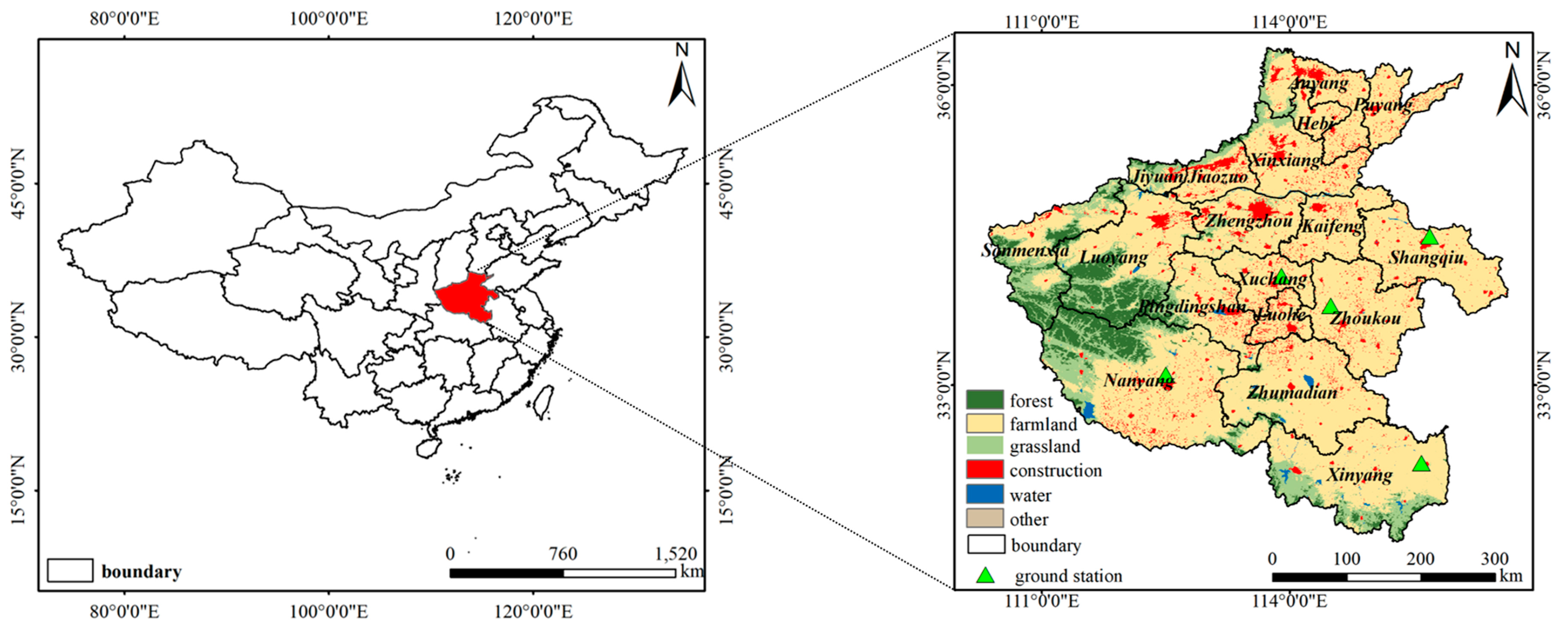
Henan Province is located in the central-eastern part of China, with geographical coordinates ranging from 31°23′ to 36°22′ N and 110°21′ to 116°39′ E, as shown in Figure 1. Influenced by the transitional zone between the northern and southern climates, most of Henan Province experiences a warm temperate semi-humid monsoon climate, while a small part in the south experiences a subtropical humid monsoon climate. The region has a dry and windy spring, a hot and rainy summer, a clear and sunny autumn, and a cold and dry winter with little rain or snow. The annual average temperature ranges between 12 °C and 16 °C, and the annual average precipitation is about 500 mm to 900 mm. Henan Province covers a total area of approximately 167,000 square kilometers, with an arable land area of approximately 10.80177 million hectares. The province contributes 10% of the national grain output and 25% of the national wheat production. Henan Province is prone to a range of climatic disasters, resulting in an annual average of 2 million hectares of crops being impacted by natural disasters [64,65,68]. Among these, agricultural droughts occur most frequently. Therefore, effective monitoring and the prevention of agricultural droughts are of great significance for promoting socio-economic development and safeguarding the well-being of individuals and their assets [64,65].

Figure 1.
Study area (the map includes the relative position of Henan Province in China and land use types).
2.2. Remote Sensing Data
2.2.1. TROPOSIF Data
Sentinel-5P is the first atmospheric monitoring satellite of the European Union’s Copernicus Earth Observation Program. It is a near-polar, sun-synchronous orbit satellite with a revisit cycle of 17 days. Equipped with the TROPOMI, it boasts a spectral resolution of 0.37 nm and an observation swath width of approximately 2600 km, enabling near-daily global surface coverage. Guanter et al. (2021) utilized the spectral windows of 743–758 nm and 735–758 nm to retrieve the SIF data using an algorithm named TROPOSIF which is based on the principal component analysis [67]. The data from this satellite is available from May 2018 to December 2021. Before August 2019, the SIF data had a spatial resolution of 3.5 km × 7 km at the nadir point, which was then improved to 3.5 km × 5 km. Due to the vulnerability of the 735–743 nm range to water vapor interference, the SIF data from the 743–758 nm window, which is not affected by water absorption lines, were chosen for analysis [69]. Frankenberg et al. (2011) developed a technique to transform the SIF data, which provides immediate information at the time of satellite overpass, into daily-scale signals by using a diurnal scaling factor. The daily-scale data for the 743–758 nm window is termed SIF_Corr_743 hereafter (http://ftp.sron.nl/open-access-data-2/TROPOMI/tropomi/sif/v2.1/l2b/, accessed on 1 October 2023) [41].
2.2.2. MODIS Data
MODIS provides long-term spectral reflectance data for vegetation cover with a spatial resolution of 500 m (https://ladsweb.modaps.eosdis.nasa.gov/, accessed on 1 October 2023). Since the reflectance obtained directly by satellites is affected by the observation angle, the MCD43A4 dataset, which is corrected by the bidirectional reflectance distribution function, was chosen for the SIF downscaling study. This dataset removes the effects of atmospheric scattering and absorption, thereby accurately reflecting the structural characteristics of SIF. We selected the reflectance data from the 620–670 nm red (b1), 841–876 nm near-infrared (b2), 459–479 nm blue (b3), and 545–565 nm green (b4) bands in the MCD43A4 dataset. Based on these reflectance data, the Soil Adjusted Vegetation Index (SAVI), NDVI, Enhanced Vegetation Index (EVI), and Near-infrared Reflectance of Vegetation (NIRv) were calculated. These indices comprehensively account for soil background, high biomass areas, and photosynthetic efficiency while avoiding oversaturation, making them effective in characterizing the structural characteristics of SIF [63]. Additionally, Leaf Area Index (LAI), Fraction of Photosynthetically Active Radiation (FPAR), and ET data were selected. FPAR is a critical component of SIF, while LAI and ET can represent physiological characteristics [58,68]. Constructing the iTFDI requires LST data. We selected the MOD11A2 dataset, which provides an 8-day composite of daytime and nighttime LST data. The LST data were resampled to a spatial resolution of 500 m using the bilinear interpolation method to match them with the downscaled SIF. The MCD12Q1 dataset provides land use type data. International Geosphere-Biosphere Programme (IGBP) standards were used to classify the land use types used in this research. Based on the experimental design, the MCD12Q1 data was reclassified into six categories: forest, farmland, grassland, construction, water, and others. The MODIS data used in the experiment is shown in Table 1. The vegetation index formulae constructed from the reflectance data are shown in Table 2.

Table 1.
MODIS data products used in the study.
Table 2.
Construction of vegetation index based on MODIS reflectance.
2.2.3. Meteorological Data
Soil moisture and precipitation data were selected to characterize the agricultural drought conditions. These data products, post-processed from the ground station data, have a spatial resolution of 1 km and a temporal resolution of 1 month. The data can be downloaded from the National Tibetan Plateau Data Center (https://data.tpdc.ac.cn/home, accessed on 28 February 2024). In order to calculate the SPEI index, data from five agricultural ground stations in Henan Province (Shangqiu, Zhoukou, Xuchang, Nanyang, and Xinyang) were downloaded from the National Meteorological Science Data Center (https://data.cma.cn/, accessed on 28 February 2024), including the latitude and longitude of each station, monthly precipitation, and monthly average temperature.
2.2.4. Complementary Data
The enhanced SIF (eSIF) data product, corrected from TROPOSIF, has a spatial resolution of 0.05° and a temporal resolution of 8 days. The monthly eSIF data for 2021 was selected to validate the accuracy of the downscaled data (https://zenodo.org/record/6115416, accessed on 20 April 2024) [62]. Drought distribution information was sourced from the Henan Provincial Hydrology and Water Resources Monitoring Center to evaluate the drought monitoring performance of the constructed iTFDI (http://www.hnssw.com.cn/, accessed on 1 May 2024).
2.3. Crop Yield Data
Crop yield data can directly assess the extent of external stress on crops. We obtained winter wheat and summer corn yield data for Henan Province from 2013 to 2022 from the National Bureau of Statistics to evaluate the relationship between the constructed iTFDI and crop yields (https://www.stats.gov.cn/, accessed on 1 May 2024).
2.4. Downscaling Model and Construction of iTFDI
2.4.1. Downscaling Model Construction
Downscaling models are commonly employed in research on LST and soil moisture to extrapolate information from one spatial scale to another [70,71,72]. In this study, the random forest algorithm was chosen, which constructs multiple decision tree learners using bagging techniques. These decision trees collectively form a random forest model [73]. The construction method of the random forest model ensures that each decision tree model possesses uniqueness, thereby mitigating overfitting to a certain extent. To arrive at its final prediction, the random forest model combines and averages all the outcomes from multiple decision trees. In addition, the random forest model ranks the selected explanatory variables and efficiently reduces data without sacrificing accuracy by calculating their contribution to the model using the Gini coefficient and out–of–bag error rate [70]. Finally, based on the assumption of the spatial scale invariance theory, the random forest downscaling model constructed using the available high-resolution explanatory variable data can improve the spatial resolution of TROPOSIF [59,63,72,74].
We used the coefficient of determination (R2), mean absolute error (MAE), and root mean square error (RMSE) as the accuracy evaluation metrics for the downscaling model [39,60,63,69].
In Equations (1)–(3), xt represents the TROPOSIF values, xp represents the predicted values, represents the mean of TROPOSIF, and n denotes the number of sample points.
2.4.2. iTFDI Construction and Drought Classification
Studies have shown that there is a triangular or trapezoidal relationship between the surface vegetation cover and the LST [75]. In light of this, Sandholt et al. (2002) proposed the TVDI for monitoring surface droughts [32].
The TVDI calculation formula is as follows:
In Equation (4), LST denotes the land surface temperature, and LSTmax and LSTmin denote the maximum and minimum land surface temperature corresponding to the same NDVI value, respectively.
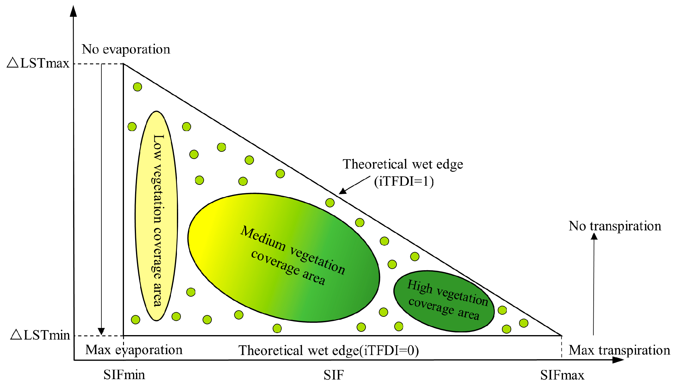
Similarly, this study introduces the iTFDI based on the downscaled SIF data. The iTFDI is built upon the idea that there is a relationship between the difference in vegetation and LST and the severity of drought in a given area. According to this hypothesis, when the soil moisture drops, the diurnal temperature range of the land surface increases, indicating a higher level of drought severity in the region [76]. The conceptual diagram of the iTFDI model is shown in Figure 2.
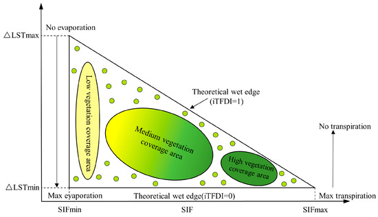
Figure 2.
The iTFDI model concept combining SIF and LST differences between day and night.
The iTFDI calculation formula is as follows:
In Equations (5)–(7), △LST denotes the land surface diurnal temperature range, and △LSTmax and △LSTmin denote the maximum and minimum diurnal temperature ranges corresponding to the same SIF value, respectively. Equations (6) and (7) define the dry and wet extremes of the model, with a and b representing the fitting coefficients for the dry extreme, and c and d representing the fitting coefficients for the wet extreme.
This study utilizes R programming to create a monthly time series of SPEI based on the Thornthwaite method. The SPEI calculation formula is as follows:
When P ≤ 0.5,
When P > 0.5, the P value is 1 − P,
In Equations (8)–(10), P is the cumulative probability weighted moment, and c0, c1, c2, d1, d2, d3 are 2.515517, 0.802853, 0.010328, 1.432788, 0.189269, 0.001308, respectively.
This study conducted a linear regression between SPEI and the corresponding iTFDI, and based on their correlation, the drought classification thresholds for iTFDI were calculated using the SPEI thresholds. Subsequently, the commonly used TVDI classification criteria were referenced and adjusted to finalize the drought classification standards for iTFDI in this study. The drought classification criteria for SPEI are shown in Table 3. Additionally, the commonly used TVDI classification criteria are shown in Table 4 [77,78,79,80]. The calculation method for the correlation coefficient (r) is shown in Equation (11), and an appropriate range is selected for drought severity classification for the iTFDI.
Table 3.
SPEI drought classification criteria.
Table 4.
Commonly used drought classification criteria for TVDI.
2.4.3. Sen’s Slope Estimator and Mann–Kendall Test
Sen’s slope estimator is a non-parametric method used to assess the trends in time series [81]. It estimates the slope of the trend line by calculating the median of the slopes of all possible pairs of data points. The formula for Sen’s slope estimator is as follows:
where i and j are the time series indices, Median denotes the median function, and β is Sen’s slope estimator. A β > 0 indicates an increasing trend in iTFDI, with a larger β reflecting a stronger increasing trend. Likewise, a β < 0 signifies a decreasing trend in iTFDI, indicating a reduction in drought conditions.
The Mann–Kendall non-parametric hypothesis testing approach is applicable for assessing data that deviate from a normal distribution. Moreover, this approach is resilient to the impact of missing data and outliers in the results of the analysis [81]. The first step is to construct the test statistic S based on the temporal iTFDI:
To construct the standardized test statistic Z:
where Var(S) represents the variance of S.
In the two-tailed trend test, given a significance level of α, the critical values are Z1−α/2 = ±1.65, ±1.96, ±2.58 for α = 0.1, 0.05, 0.01, respectively. In the case of |Z| > 1.65, 1.96, and 2.58, the trend is considered statistically significant at the 90%, 95%, and 99% confidence levels, respectively. The method for determining trend significance is shown in Table 5.
Table 5.
Trend significance determination method.
3. Results
3.1. TROPOSIF Downscaling Model and Results
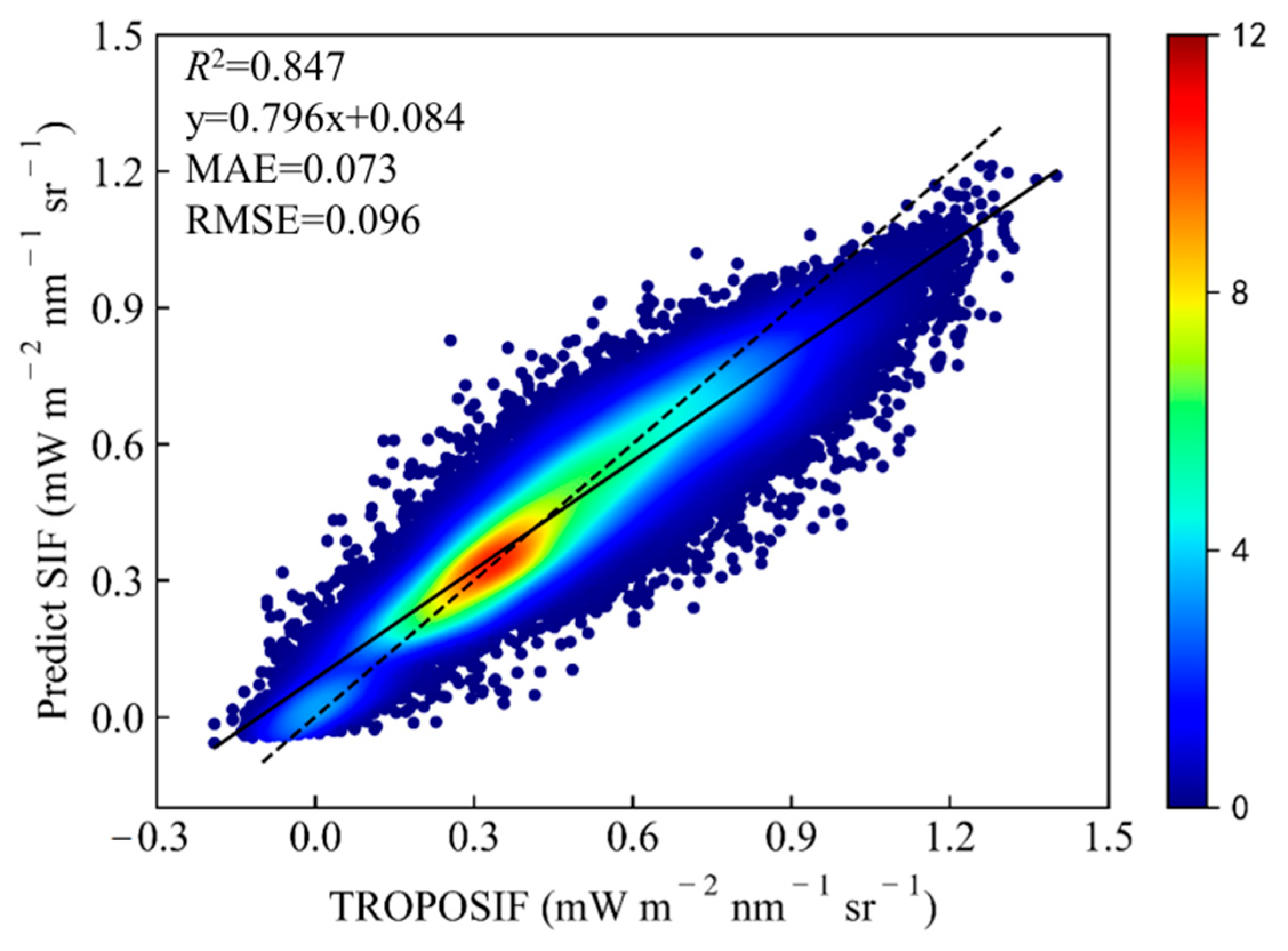
The monthly average data was synthesized from the TROPOSIF dataset for the months of March to September 2018–2021. Data for explanatory variables with the same spatial resolution were extracted using the location information of TROPOSIF. A random forest model was used to rank the importance of the explanatory variables as shown in Table 6. In order to reduce data redundancy, the top seven characteristic variables were selected as explanatory variables for the TROPOSIF downscaling, and a random forest downscaling model was constructed. With the training set and testing set accounting for 70% and 30% of the sample size, respectively, the model achieved accuracy metrics of R2 = 0.847, MAE = 0.073 mW m−2 nm−1 sr−1, and RMSE = 0.096 mW m−2 nm−1 sr−1 (as shown in Figure 3), which fully meets the downscaling requirements.
Table 6.
The importance of evaluation of explanatory variables based on random forest algorithm.
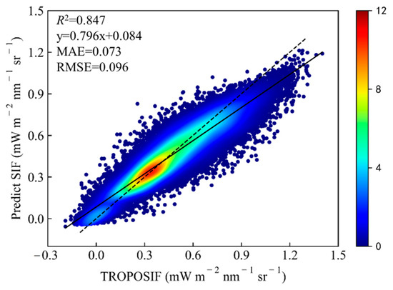
Figure 3.
The accuracy of random forest downscaling model of TROPOSIF spatial resolution.
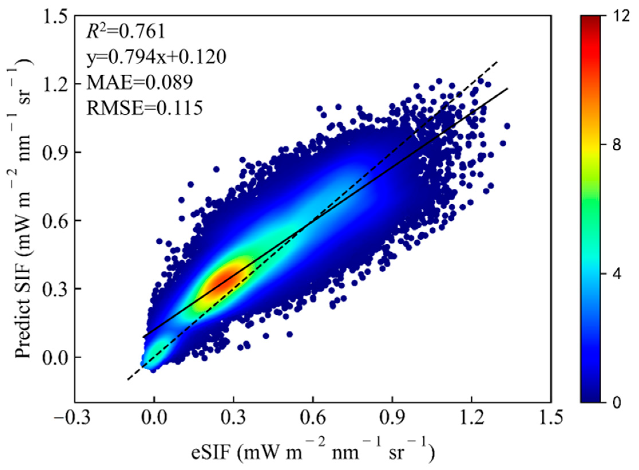
To verify the reliability of the downscaling model, we resampled the downscaled iSIF data from March to September of 2021 to a spatial resolution of 0.05° and performed a spatial correlation analysis with the eSIF data [62]. This approach evaluates the performance of the downscaling model across different spatial resolutions and ensures its reliability for practical applications.
According to Figure 4, the R2, MAE, and RMSE between the downscaled SIF and eSIF data are 0.761, 0.089 mW m−2 nm−1 sr−1, and 0.115 mW m−2 nm−1 sr−1, respectively. These results indicate that the SIF results obtained from the experimental model have a good correlation with the eSIF data, validating the effectiveness of the downscaling model constructed in this study.

Figure 4.
Verification of the downscaling model using eSIF data from March to September of 2021.
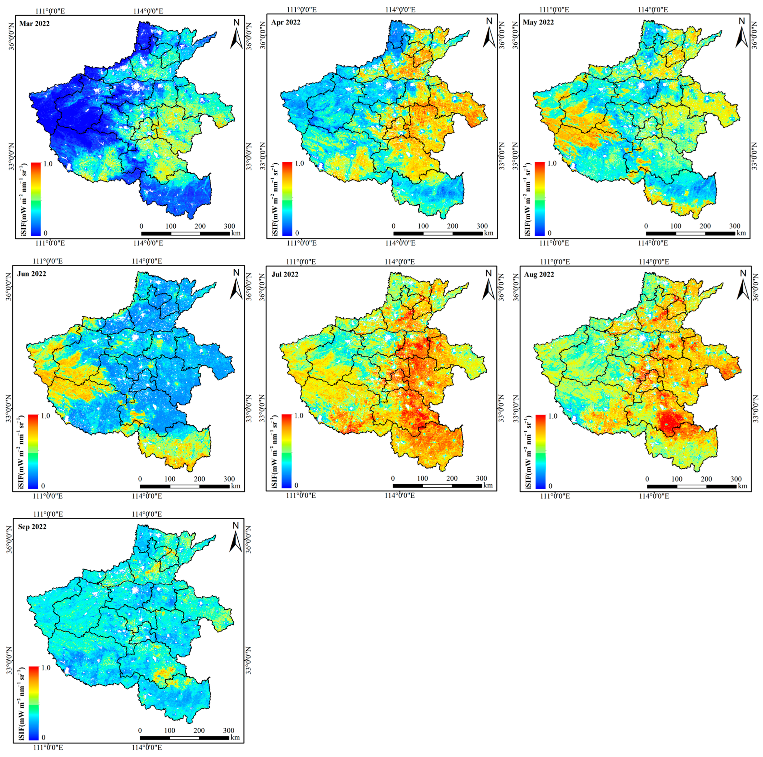
Based on the constructed random forest downscaling model and the theory of invariant spatial scale relationships, the 500 m monthly explanatory variable data were used to retrieve the 500 m monthly SIF data for Henan Province from March to September of 2010–2022, referred to as improved SIF (iSIF). The results of the iSIF for the year 2022 are shown as an example in Figure 5. Due to the absence of the 2022 data product for TROPOSIF, the 2021 data from the same period were used for comparative analysis, as shown in Figure 6.

Figure 5.
The monthly mean 500 m spatial resolution iSIF data after downscaling from March to September of 2022.
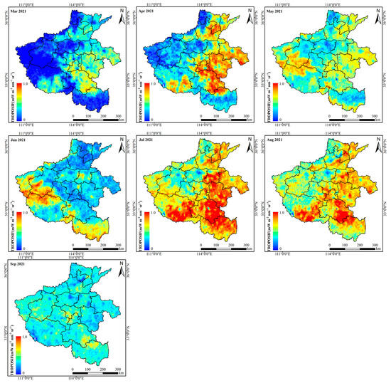
Figure 6.
The monthly mean TROPOSIF data from March to September of 2021.
By comparing Figure 5 and Figure 6, it can be seen that the high SIF values were mainly concentrated in the agricultural areas from March to April. After May, SIF values in agricultural areas started to decrease, with high values concentrated in the western mountainous regions. This change was primarily due to the maturation of winter wheat in May, which reduces chlorophyll content and leads to a decline in SIF values. Conversely, the forested areas in the western mountains are in a vigorous growth stage, resulting in relatively high SIF values. In Henan Province, the summer crop planting structure is complex, with summer corn being the main crop. In June, which is the time for harvesting winter wheat and planting summer corn, SIF values for agricultural areas reach their lowest during the study period. Starting from July, as summer corn plants grow vigorously, SIF values increase significantly and reach their annual peak. In September, as fall approaches, the vitality of plants substantially decreases, and the SIF values decrease significantly across the province. By comparison, it is evident that the downscaled 500 m monthly iSIF exhibited a similar variation trend to the coarse-resolution TROPOSIF, but iSIF can capture changes in more detail.
3.2. Drought Classification and iTFDI Result Verification
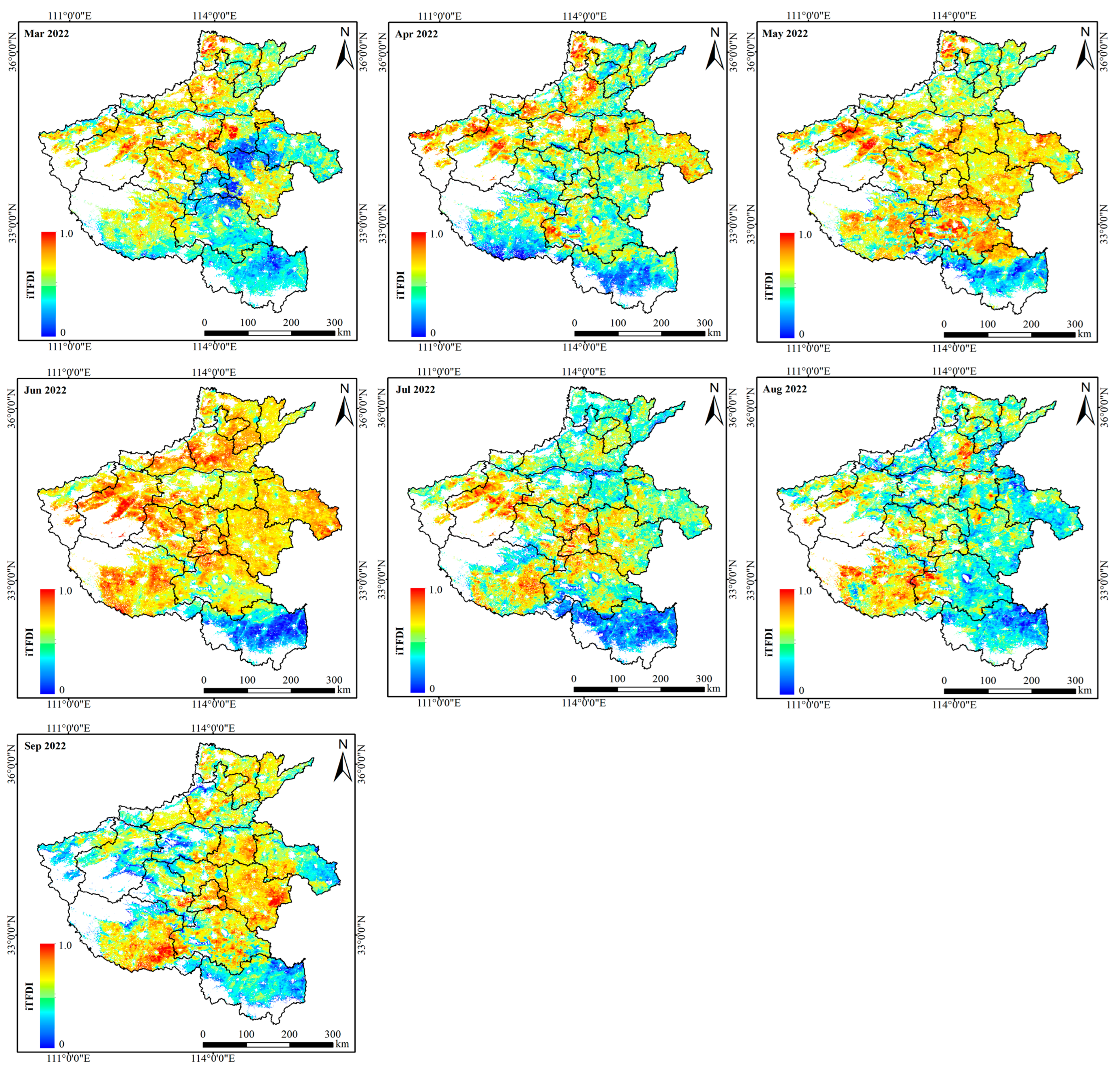
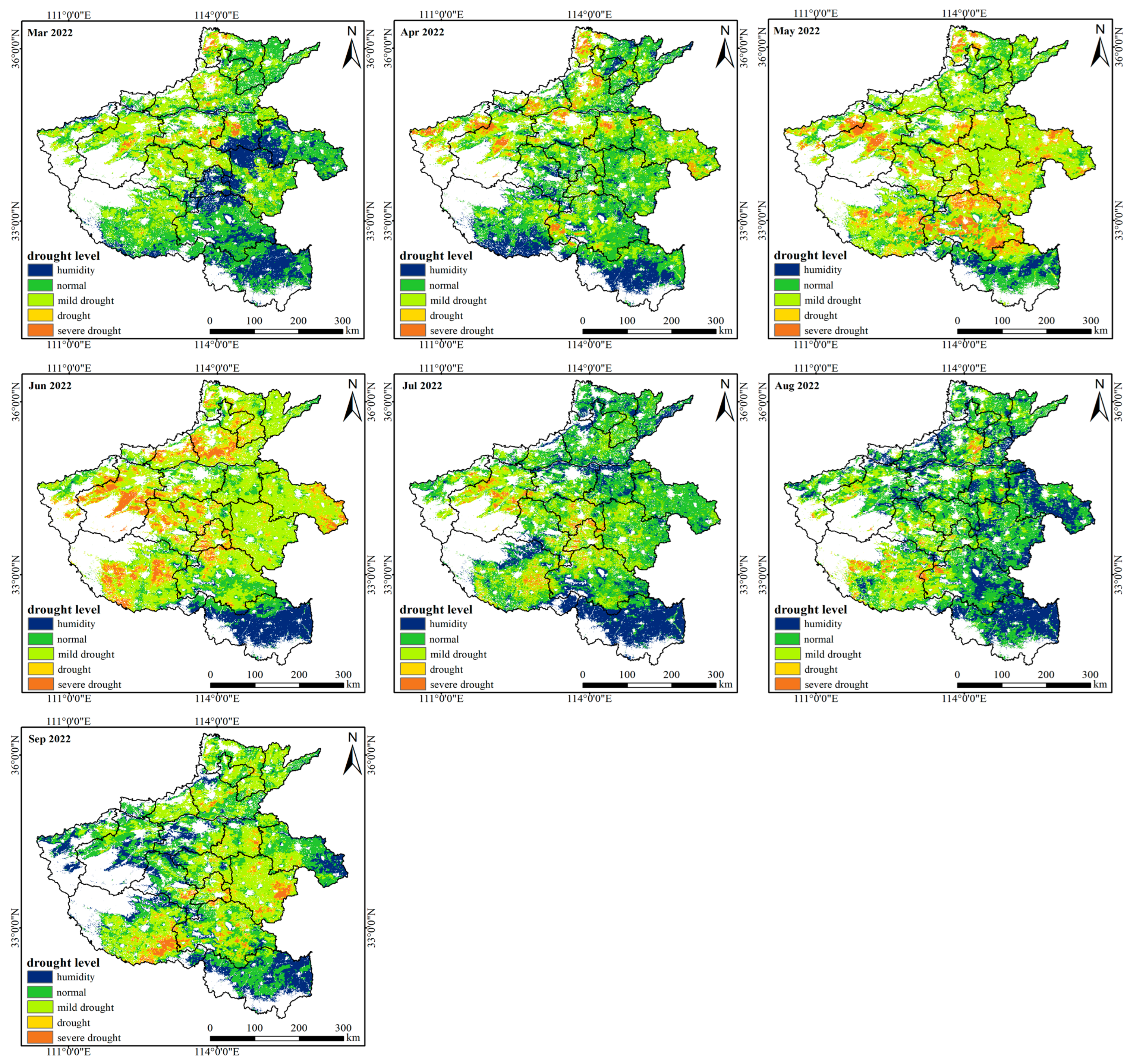
Based on the iTFDI construction method, the drought monitoring index iTFDI for Henan Province was ultimately constructed. The iTFDI values range from 0 to 1. Lower iTFDI values correspond to areas with less drought stress, while higher iTFDI values indicate more severe drought conditions. The iTFDI data for Henan Province from March to September 2022 is presented in Figure 7.
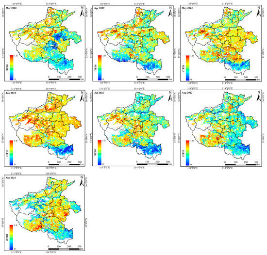
Figure 7.
The iTFDI values are retrieved by combining iSIF and LST difference data from March to September of 2022.
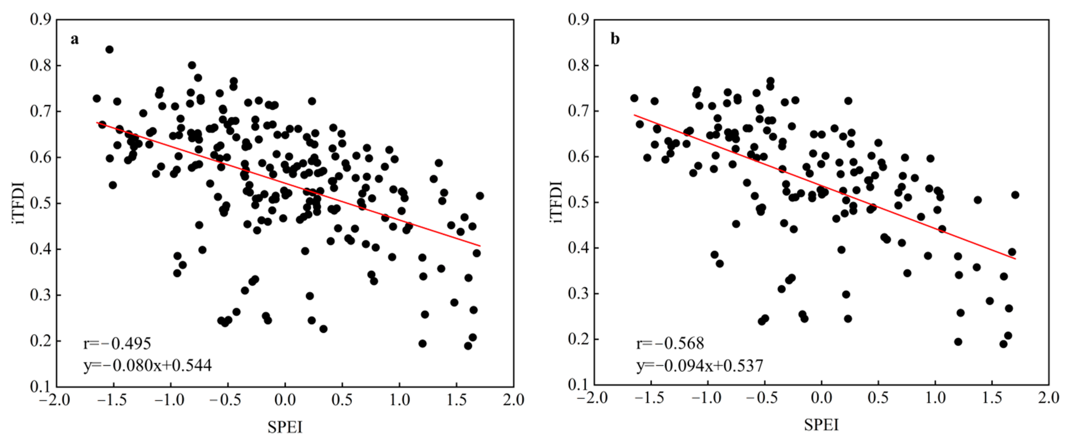
We constructed a monthly-scale SPEI from five agricultural meteorological stations in Henan Province from 2010 to 2021. The iTFDI data was extracted by utilizing the station’s location information and building a fitting relationship with SPEI. The fitting results are shown in Figure 8a. The analysis revealed a correlation of −0.495 between the ground station SPEI data and iTFDI. However, after fitting was performed for the months of June, July, August, and September, the correlation increased to −0.568. As can be seen in Figure 8b, there is a clear inverse relationship between ground station SPEI data and iTFDI. This fitting method can help determine the classification standards for the iTFDI drought levels, making the iTFDI drought monitoring more operational and accurate in practice.
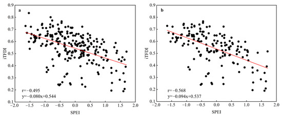
Figure 8.
Correlation between iTFDI and ground station SPEI. (a) fitting results from March to September; (b) fitting results for March, May, June, and July.
The fitting regression lines of ground station SPEI and iTFDI for the months of March, May, June, and July were used to derive the iTFDI thresholds that correspond to the SPEI thresholds. Table 7 shows the derived iTFDI drought classification thresholds. This study indicates that the fitted iTFDI closely matches the classification criteria of levels 2 and 4 in Table 4. Therefore, after a comprehensive comparison, the final drought classification criteria were determined as shown in Table 7.
Table 7.
Experimental fitting and determined iTFDI drought grade classification criteria.
Based on the drought classification levels determined from the experiment, Figure 9 and Table 8 show the distribution map of the iTFDI drought severity and the proportion of drought levels for agricultural lands in Henan Province from March to September of 2022. From Figure 9 and Table 8, it can be seen that Henan Province generally had suitable soil moisture during the study period in 2022. However, various degrees of drought occurred in some localities in March, April, July, and August, while large-scale droughts of varying degrees occurred in May, June, and September.
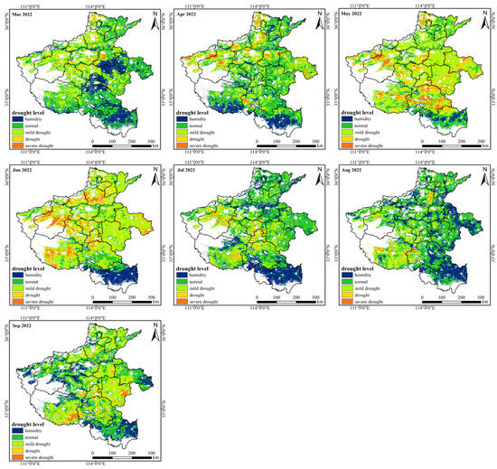
Figure 9.
Classification results of the iTFDI drought levels from March to September of 2022.
Table 8.
Proportion of iTFDI drought levels for agricultural lands from March to September of 2022.
According to Figure 9 and Table 8, the most severe droughts in 2022 occurred in May and June. Based on the iTFDI drought classification in May, Henan Province showed an overall mild drought condition. The primary factors contributing to this phenomenon were the increasing temperatures, comparatively reduced rainfall in comparison to other months, and the winter wheat being in its advanced development phase, resulting in decreased irrigation. Consequently, the province experienced an overall mild drought, with some severe droughts in localized areas. Nevertheless, a widespread and severe drought occurred in the mid-western regions of Luoyang, eastern Sanmenxia, and Zhumadian. The June iTFDI drought classification showed mild drought with severe drought areas spreading westward, especially damaging Xuchang, Pingdingshan, Nanyang, Xinxiang, Jiaozuo, and Luoyang, where the drought worsened and spread. Meanwhile, the severe drought areas in Shangqiu, Zhoukou, and Zhumadian in the east were alleviated to some extent. In May-June, Xinxiang experienced a notable shift in drought conditions, transitioning from a mild to a severe drought. Xinyang remained drought-free during this period.
According to the hydrological and water resources information released by the Henan Province Hydrological and Water Resources Monitoring Center (http://www.hnssw.com.cn/, accessed on 1 May 2024), the soil moisture conditions in Henan Province were suitable in March, April, and July 2022, with no significant drought occurrences (http://www.hnssw.com.cn/l1SwfwL2Sqxx/34412.jhtml, http://www.hnssw.com.cn/l1SwfwL2Sqxx/34411.jhtml, http://www.hnssw.com.cn/l1SwfwL2Sqxx/34408.jhtml, accessed on 1 May 2024). The iTFDI, as created in this work, confirms that the soil moisture conditions during this period were favorable, with no notable drought. This finding aligns well with the published information, indicating a high level of agreement. Conditions for soil moisture were favorable across the province at the beginning of May. However, due to the high temperatures and low precipitation in the middle and late periods of the month, varying degrees of drought occurred across the province. Notably, a severe drought was observed in Anyang, Xinxiang, Puyang, Kaifeng, Luoyang, Pingdingshan, Xuchang, Zhoukou, and Zhumadian, while a mild drought was observed in Jiaozuo, Nanyang, Shangqiu, Xinyang, and Sanmenxia (http://www.hnssw.com.cn/l1SwfwL2Sqxx/34410.jhtml, accessed on 1 May 2024). In general, the iTFDI-reflected drought areas agreed with the reported drought areas, with the exception of a few discrepancies caused by favorable soil moisture conditions in early May and the later occurrence of drought in various regions to varying degrees. In June, the water information indicated widespread and persistent high temperatures across the province, leading to severe soil moisture depletion. A severe drought was observed in Anyang, Xinxiang, Jiaozuo, Sanmenxia, Luoyang, Xuchang, Luohe, Pingdingshan, and Nanyang (http://www.hnssw.com.cn/l1SwfwL2Sqxx/34409.jhtml, accessed on 1 May 2024), which is highly consistent with the drought distribution detected by the iTFDI. In August, the water information indicated that different degrees of drought occurred in the southern part of Henan Province in the month’s latter half, mainly concentrated in Sanmenxia, Luoyang, Nanyang, Zhengzhou, Pingdingshan, Kaifeng, Zhoukou, Zhumadian, and Xinyang (http://www.hnssw.com.cn/l1SwfwL2Sqxx/34407.jhtml, accessed on 1 May 2024). The monthly iTFDI showed a mild drought in the southern part of Henan Province, with favorable overall soil moisture conditions in other areas, which is consistent with the spatial distribution of the published water information. In September, the water information indicated a significant decrease in precipitation compared to the normal level, leading to varying degrees of drought. Specifically, the soil moisture conditions in Pingdingshan, Nanyang, and Zhumadian were relatively poor, with more pronounced drought conditions observed. A mild drought was observed in Anyang, Jiaozuo, Luoyang, Luohe, and Zhoukou (http://www.hnssw.com.cn/l1SwfwL2Sqxx/34406.jhtml, accessed on 1 May 2024), which aligns well with the drought areas detected by the iTFDI.
By comparing the drought levels monitored by the iTFDI for 2022 with the drought area distribution reported by the Henan Province Hydrological and Water Resources Monitoring Center, it is evident that there is a high degree of consistency between the two datasets. This indicates that the iTFDI can provide a scientific basis for agricultural production and water resource management, effectively supporting the formulation of drought early warning and mitigation measures. It also demonstrates that the downscaled iSIF data can be applied for drought monitoring.
3.3. iTFDI Trend Analysis and Testing
This study employed the Sen’s slope estimator and Mann–Kendall test to examine the trend in the iTFDI data for agricultural land in Henan Province from March to September of 2010–2022. The objective was to investigate the patterns of drought situations over time. The results of the trend analysis for different significance levels are illustrated in Figure 10.
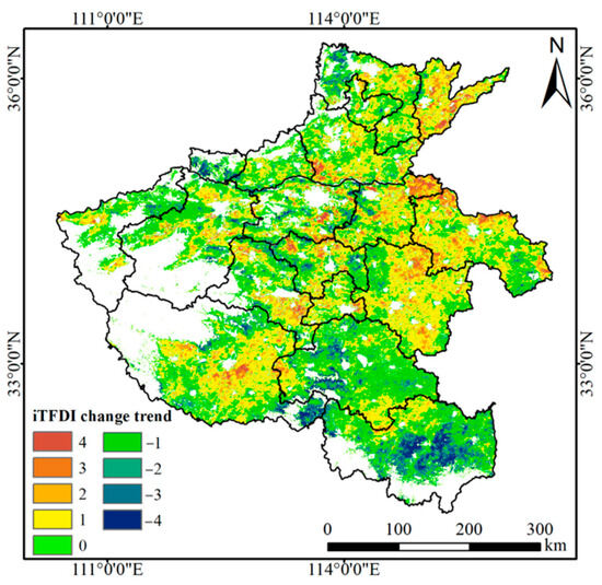
Figure 10.
The annual trend analysis and significance test results of agricultural land from 2010 to 2022.
Based on the data from Table 5 and Figure 10, the agricultural land area in Henan Province, where the Sen’s slope estimate for the iTFDI indicates a rising pattern, makes up 46.06% of the overall area. This tendency was primarily observed in Puyang, Anyang, Xinxiang, Kaifeng, Shangqiu, Zhoukou, and Nanyang. Among these regions, the areas passing the significance tests at α = 0.01, α = 0.05, and α = 0.1 levels were 1.31%, 3.38%, and 4.0%, respectively. The significant regions are primarily located in the eastern part of Puyang, the southwestern part of Xinxiang, the northeastern part of Kaifeng, the northern part of Shangqiu, and the central part of Nanyang, exhibiting a pattern of minor occurrences around areas of extreme significance. The area with a non-significant increasing trend for the iTFDI accounts for 37.38% of the total area. Additionally, the area where the iTFDI shows a decreasing trend occupies 43.94% of the total area, with the trend mainly observed in the western part of Anyang, Jiyuan, the eastern part of Sanmenxia, the eastern and western parts of Luoyang, the eastern and western parts of Zhengzhou, the eastern part of Shangqiu, the eastern and western parts of Xuchang, the northern part of Pingdingshan, the northern and southern parts of Nanyang, as well as Zhumadian and Xinyang. Among these regions, the areas passing the significance tests at α = 0.01, α = 0.05, and α = 0.1 levels were 2.28%, 4.46%, and 4.02% of the total area, respectively, with significant regions concentrated in the western part of Anyang, Jiyuan, the northern and southeastern parts of Nanyang, the western part of Zhumadian, and most of Xinyang. The area with a non-significant decreasing trend for the iTFDI accounts for 33.19% of the total area. Additionally, the area where the iTFDI trend shows no change constitutes 10% of the total area. In summary, the annual Sen’s slope and Mann–Kendall significance test revealed a significant decreasing trend in drought severity in the southern and western regions of Henan Province, while the eastern region showed a significant increasing trend.
3.4. Comparison of TVDI and iTFDI
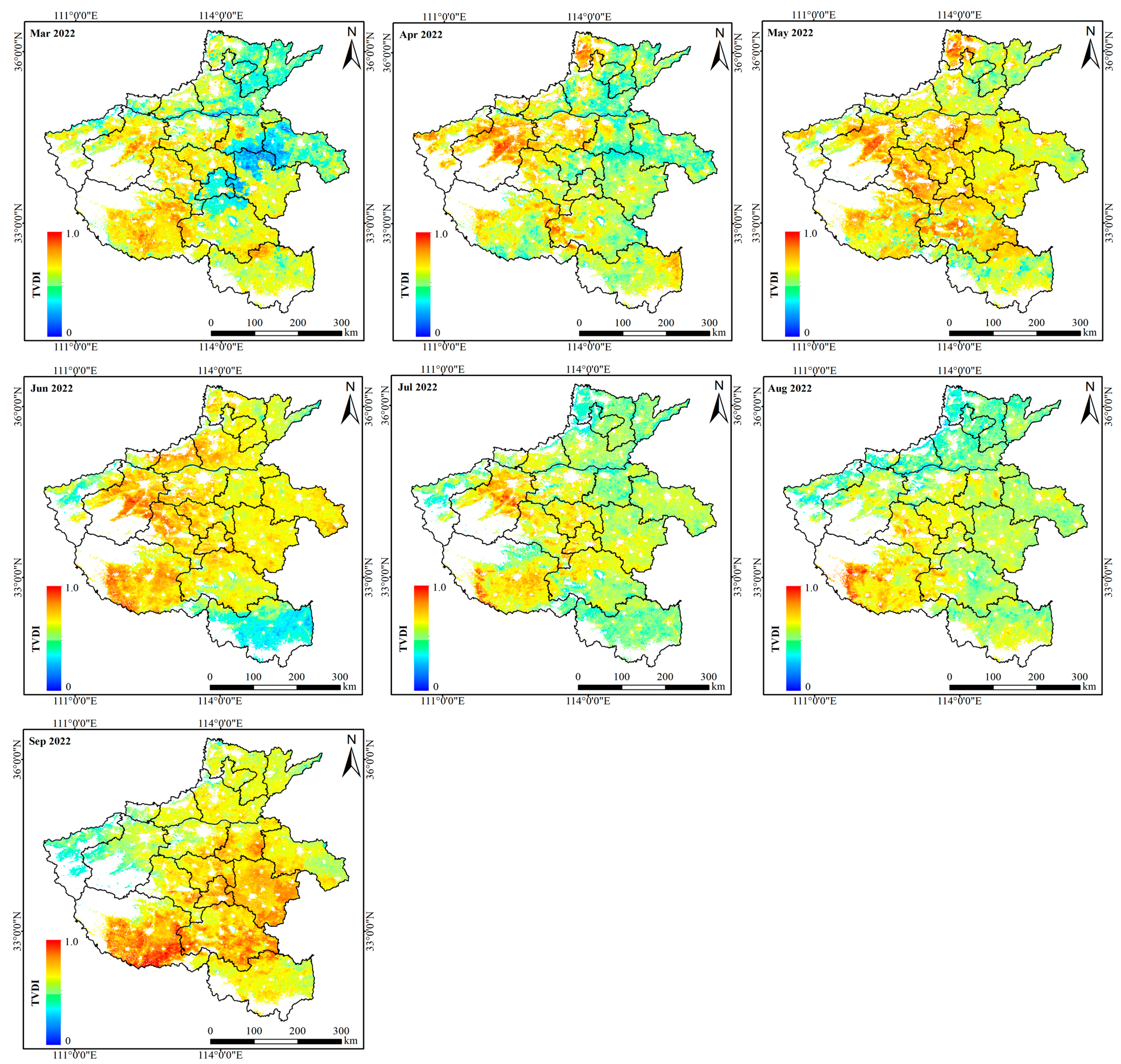
The TVDI is a mature remote sensing drought monitoring method commonly used to assess the spatial distribution of drought-affected areas, particularly in agricultural drought monitoring studies. Comparing the spatial distribution of TVDI and iTFDI indices can validate the effectiveness of the constructed iTFDI index. We used the 2022 TVDI data product to compare and analyze the spatial distribution of the iTFDI data.
By comparing Figure 7 and Figure 11, it can be seen that iTFDI and TVDI exhibit similar spatial distribution trends, consistent with the water condition information published by the Henan Hydrology and Water Resources Center. This indicates that both methods perform well in monitoring drought events. However, during the periods of relatively good soil moisture conditions in March, April, and July, while both TVDI and iTFDI show high values in certain local areas, TVDI has far greater high-value regions compared to iTFDI. In contrast, during the drier months of May, June, and September, both indices show varying degrees of drought across most of the province. Notably, in August, iTFDI provides a more accurate reflection of severe drought conditions in the northern part of Sanmenxia City. Overall, while both iTFDI and TVDI perform satisfactorily in monitoring drought conditions, the iTFDI demonstrates a superior drought monitoring capability for certain local areas.
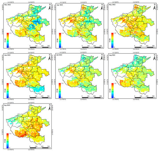
Figure 11.
Monthly mean TVDI data from March to September of 2022.
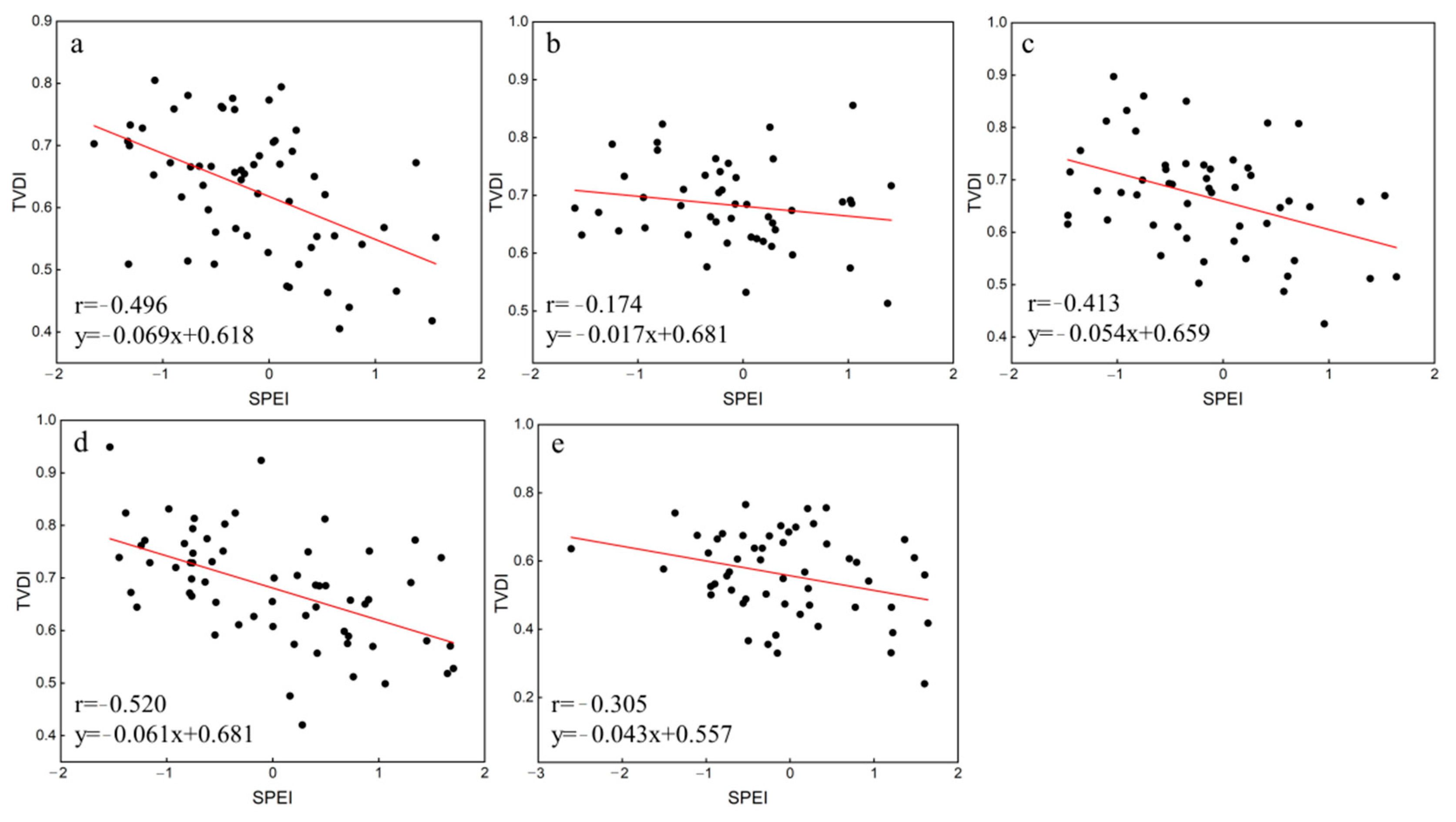
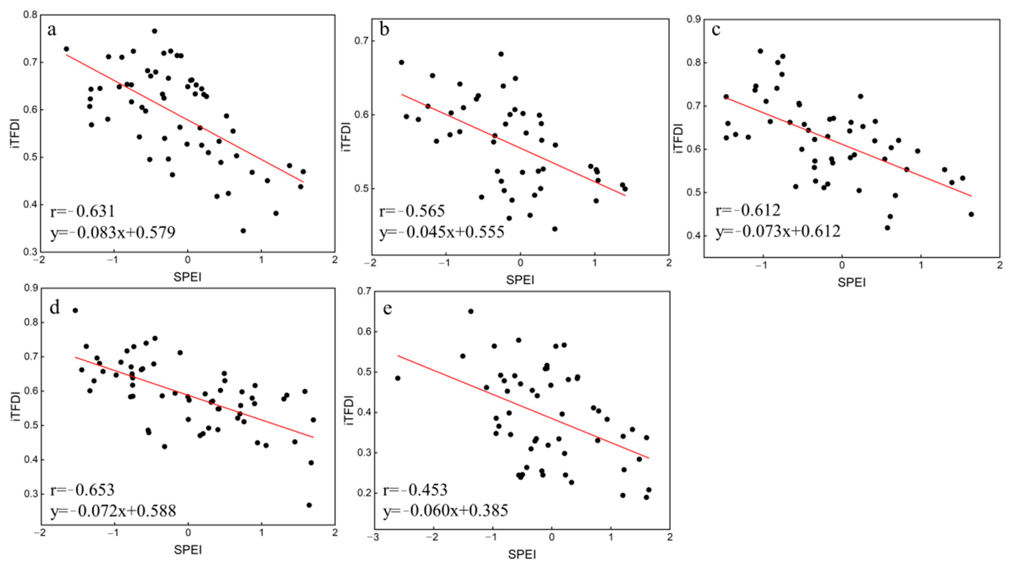
We used the SPEI data from five stations to verify the correlation with TVDI and iTFDI, and the results are shown in Figure 12 and Figure 13. By comparing these figures, it can be seen that the constructed iTFDI index shows a better correlation with SPEI compared to the TVDI index. Additionally, the correlation between the iTFDI and SPEI is approximately 0.6, indicating a weaker correlation significance. This is mainly due to the fact that SPEI is based on point data while the iTFDI data has a spatial resolution of 500 m, leading to potential discrepancies due to scale differences.
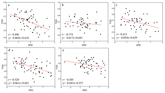
Figure 12.
The correlation between SPEI and TVDI for five ground stations. (a) Shangqiu Station; (b) Zhoukou Station; (c) Xuchang Station; (d) Nanyang Station; (e) Xinyang Station.
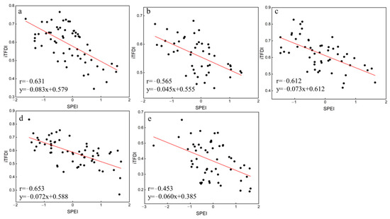
Figure 13.
The correlation between SPEI and iTFDI for five ground stations. (a) Shangqiu Station; (b) Zhoukou Station; (c) Xuchang Station; (d) Nanyang Station (e) Xinyang Station.
3.5. Relationship between Meteorological Data and iTFDI
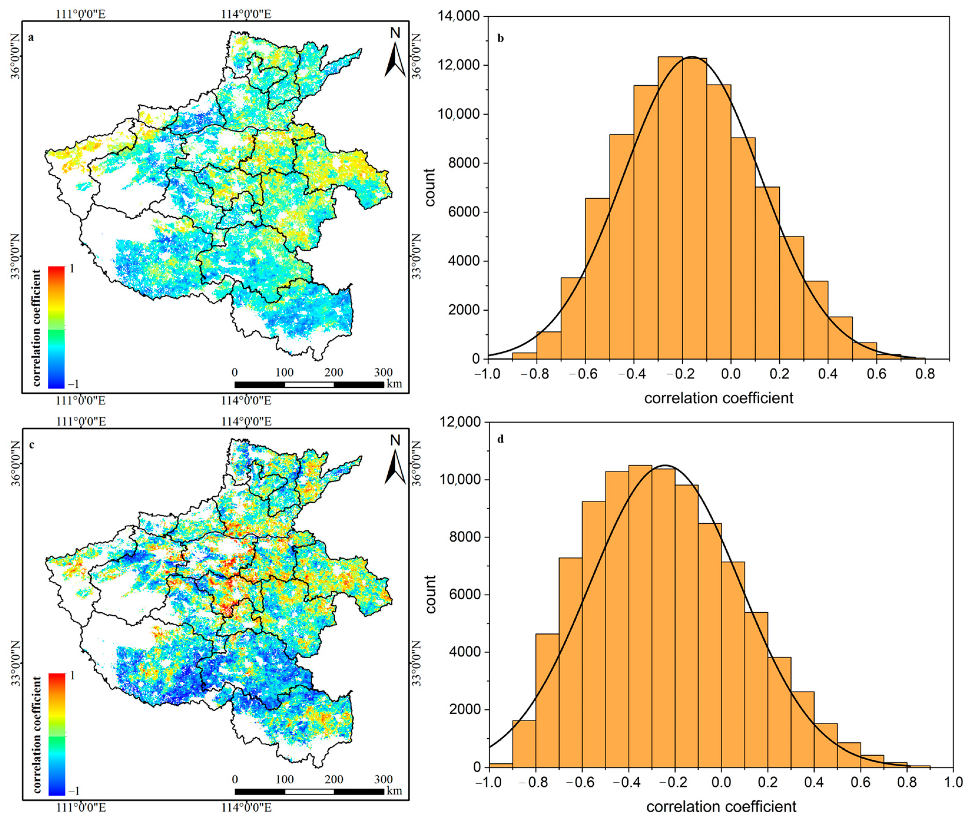
Increased precipitation and soil moisture can effectively alleviate agricultural drought conditions. This study evaluates the correlation between meteorological data and the constructed iTFDI based on mean annual precipitation and soil moisture data from March to September of 2010–2020.
From Figure 14, it can be seen that the correlation between precipitation and soil moisture with the iTFDI is relatively weak. Figure 14a shows that there is a certain negative correlation between precipitation and iTFDI in the southern region of Henan Province and the northern area of Jiaozuo City, but no significant correlation is found in other regions overall. Figure 14b indicates that, although the correlation coefficient generally shows negative values, the correlation is weak, suggesting that the relationship between precipitation and iTFDI is not significant. Figure 14c demonstrates that the areas with a strong negative correlation between soil moisture and iTFDI are mainly concentrated in the southeastern part of Nanyang City, the northern part of Xinyang City, and Zhumadian City, while other regions exhibit lower correlations. However, certain localized areas show a noticeable positive correlation. Figure 14d reveals that the overall correlation between soil moisture data and iTFDI is negative, with a peak correlation value of approximately −0.4. In conclusion, there is no significant correlation between iTFDI values and precipitation or soil moisture during the same period.
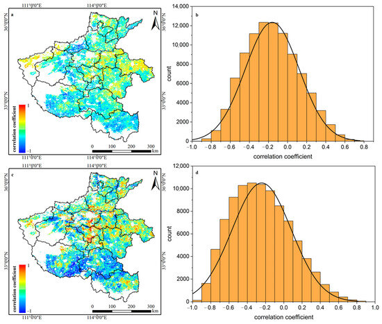
Figure 14.
The spatial correlation between iTFDI and meteorological data from 2010 to 2020. (a) correlation with precipitation; (b) histogram of precipitation; (c) correlation with soil moisture; (d) histogram of soil moisture.
3.6. Relationship between iTFDI and Crop Yields
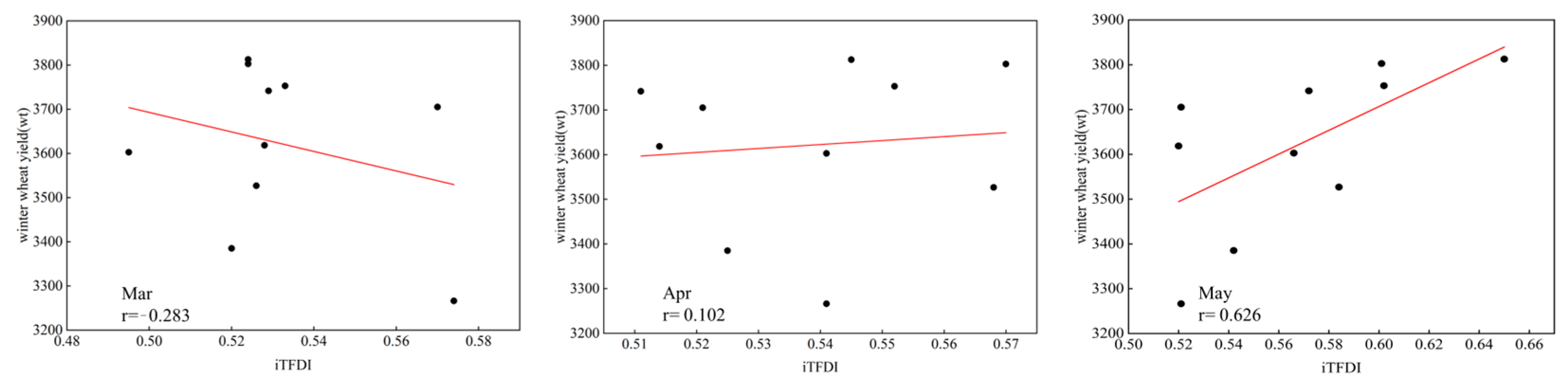
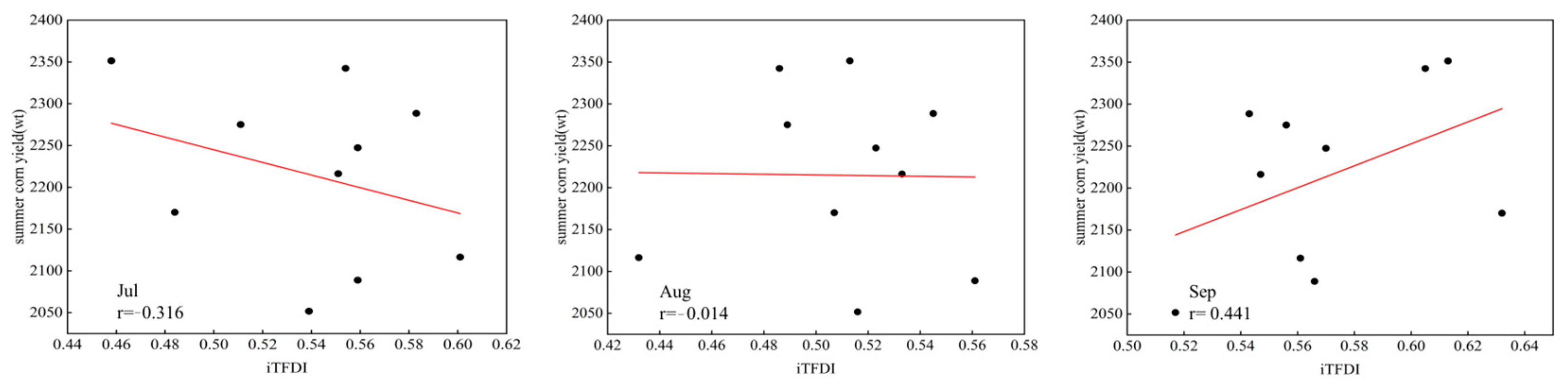
Drought directly affects crop yield and historical crop yield data can be used to evaluate the effectiveness of the agricultural drought monitoring methods. This study analyzed the correlation between the monthly average iTFDI from 2013 to 2022 and the yield of winter wheat (March–May) and summer corn (July–September). Figure 15 and Figure 16 show the correlation between iTFDI and the yields of winter wheat and summer corn.
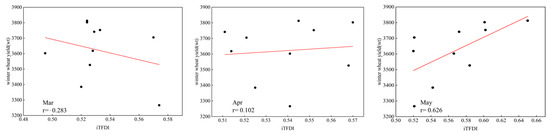
Figure 15.
Correlation between iTFDI and winter wheat yield from March to May in 2013–2022.
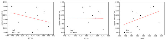
Figure 16.
Correlation between iTFDI and summer corn yield from July to September in 2013–2022.
According to Figure 15, the correlation coefficients for the iTFDI and winter wheat yield in March and April are −0.283 and 0.102, respectively, indicating no significant correlation between them. However, in May, as winter wheat enters the maturation stage, the correlation between the iTFDI and the crop yield increases significantly, with r reaching 0.626, demonstrating a strong correlation.
According to Figure 16, the correlation coefficients between the iTFDI and the summer corn yield in July and August are −0.316 and −0.014, respectively, indicating no significant correlation. However, in September, as summer corn reaches its maturation stage, the correlation between the iTFDI and the crop yield strengthens, with r reaching 0.441, indicating a moderate positive correlation.
Comparing the monthly correlation between the iTFDI and the yields of winter wheat and summer corn reveals no significant correlation during the early growth stages of the crops. However, during the maturation period of the crops, the iTFDI demonstrates a strong correlation with the crop yield. This indicates that iTFDI is an effective agricultural drought monitoring indicator, particularly during critical growth periods such as maturation, where it can effectively reflect the impact of drought on crop yields.
4. Discussion
4.1. Limitations of Drought Monitoring Method Combined with SIF
Downscaling methods based on the assumption of invariant spatial scale relationships have been widely applied to improve the spatial resolution of surface temperature, soil moisture, and precipitation data [70,71,72]. To effectively downscale the SIF data products, it is essential to understand the underlying causes of SIF variations and select reliable variable data to represent the changes in SIF information.
where PAR represents the photosynthetically active radiation, FPAR is the fraction of photosynthetically active radiation absorbed by vegetation, fesc denotes the SIF escape probability, and SIFyield refers to the fluorescence quantum yield.
Based on Equation (16), the SIF is determined by both the structural and physiological characteristics of vegetation. In selecting explanatory variables, the study fully considered the characteristics of SIF, choosing commonly used reflectance and vegetation index data to represent structural characteristics [58,59,60], while also selecting LAI and meteorological data such as ET to represent physiological characteristics [58,68]. Although these characteristics were considered during the reconstruction of SIF, the SIF data reconstructed based on the theory of spatial scale invariance may still experience some degree of distortion and cannot fully reflect the true SIF [58,59,60,61,62,63]. Therefore, utilizing satellite data to directly obtain higher spatial resolution SIF products could further improve the performance of drought monitoring. The accuracy of drought classification directly affects the experimental results. However, some studies have not adequately considered whether existing drought classification standards are applicable to the improved indices [64,65]. This is especially true for the TVDI index, where classification standards vary across different regions [77,78,79,80]. Sha S et al. (2014) pointed out that establishing a relationship between TVDI and soil moisture can improve the accuracy of TVDI-based drought classification, but the drought degree represented by soil moisture content is still unclear [82]. Chen S et al. (2017) conducted a spatiotemporal analysis of drought in Henan Province using SPEI and TVDI, finding a good correlation between the two [83]. Therefore, fitting station-based SPEI data with iTFDI is a feasible approach, but the limited number of station-based SPEI data and the significant spatial scale differences with iTFDI result in low data correlation. Selecting data from months with better performance to replace annual data and adjusting according to commonly used TVDI classification standards can improve the accuracy of iTFDI drought classification. If possible, obtaining more station-based SPEI data could further enhance the accuracy of drought classification [83].
4.2. Trends of Downscaling and Drought Monitoring Results
The importance of these explanatory variables was ranked using a random forest model. The ranking shows that b2 and NIRv have high importance scores, consistent with current research indicating that b2, NDVI, and NIRv are effective in characterizing SIF [62,69]. By comparing the correlations of the reconstructed monthly average iSIF with NDVI and EVI (as shown in Figure 17), the correlation coefficients are 0.844 and 0.946, respectively. According to Table 6, although the importance of EVI and NDVI is not significant during the downscaling process, the downscaled iSIF still shows a significant correlation with both NDVI and EVI. These findings are consistent with the results validated by Yu L and Zhang Z at a 0.05° spatial scale [60,64].
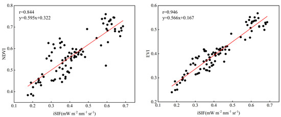
Figure 17.
Correlation between downscaled iSIF and NDVI, EVI for Henan Province from March to September of 2010–2022.
According to the iTFDI constructed from iSIF and LST difference data, the drought monitoring results for 2022 are consistent with the data published by the Hydrology and Water Resources Monitoring Center of Henan Province, demonstrating the effectiveness of the iTFDI and its drought classification. Additionally, the drought trend in Henan Province from 2010 to 2022 shows a significant decrease in the south and west, while an increasing trend is observed in the east. Overall, the intensity of drought across the province is declining. These findings are consistent with the spatiotemporal variations observed in drought monitoring results conducted by Zhang Z et al. (2023) based on SIF [84]. The study also found a weak correlation between annual precipitation and soil moisture with iTFDI values, mainly due to the potential lag of iTFDI in response to precipitation and soil moisture [34,35,65]. Moreover, factors such as annual data averaging, short study periods, and data anomalies caused by artificial irrigation can also affect the correlation between the data. Studying the lag between iTFDI and drought conditions and obtaining farmland irrigation data may better explore the relationship between iTFDI and meteorological data. Overall, the spatial distribution of drought monitored by iTFDI in Henan Province aligns with the official drought information (http://www.hnssw.com.cn/l1SwfwL2Sqxx/index_2.jhtml, accessed on 1 May 2024), indicating that the iTFDI can be applied to agricultural drought monitoring in Henan Province.
4.3. Agronomic Significance of the iTFDI Results
SIF can capture the physiological responses of vegetation earlier and more accurately than traditional vegetation indices [34]. The reconstruction of TROPOSIF based on the theory of spatial scale invariance provides data support for the application of SIF at higher spatial scales. The study found that the reconstructed iSIF better represents the growth status of vegetation; however, the iTFDI constructed from iSIF shows limited advantages in agricultural yield estimation, with only certain correlations during the crop maturation stage. Zhang Z et al. (2021) research also demonstrated that drought indices have a weak correlation with crop yield [64]. This is mainly due to the significant variations in indicators representing vegetation growth status at different growth stages. As an indicator for assessing crop drought, the iTFDI tends to show no drought during the growing season in Henan Province due to factors such as artificial irrigation, making it difficult to effectively evaluate crop yield using regional averages. However, the iTFDI exhibits higher sensitivity and timeliness in spatial drought monitoring compared to the commonly used TVDI. Zhang Z et al. (2021) also showed in their drought monitoring in the North China Plain that the integration of new global SIF (GOSIF) data can better capture drought variations [64]. The Comprehensive Drought Monitoring Index (CDMI) constructed by Zhang Z et al. (2021) using SIF data has also demonstrated higher reliability in drought monitoring in Henan Province [85]. These studies confirm that drought indices constructed with SIF can capture the physiological changes of crops under water stress earlier and more accurately than traditional vegetation indices, providing timely warning information for agricultural management departments and promoting sustainable agricultural development.
5. Conclusions
Remote sensing can quickly monitor agricultural drought severity, but traditional vegetation indices for drought monitoring have a long lag time, making early drought warning impossible. As a proxy for photosynthesis, SIF holds great promise for drought monitoring and can directly reflect changes in vegetation. However, the SIF data is limited with its low spatial resolution and spatial discontinuity, making it unsuitable for direct application in drought monitoring. This study aimed to address the issue of low spatial resolution of TROPOSIF and to develop a new drought index for crop drought monitoring. The research, based on the theory of spatial scale invariance and the vegetation–surface temperature difference hypothesis, improved the spatial resolution of SIF and constructed the iTFDI. The main conclusions are as follows:
- A random forest downscaling model was developed in this study based on the TROPOSIF data and MODIS b2, NIRv, ET, EVI, SAVI, b4, and LAI data. This model achieved an accuracy of R2 = 0.847, MAE = 0.073 mW m−2 nm−1 sr−1, and RMSE = 0.096 mW m−2 nm−1 sr−1. The study successfully inverted a 500 m spatial resolution iSIF data product for March to September of 2010 to 2022.
- We created the iTFDI by combining iSIF with surface temperature differential data. The monthly drought severity study conducted in 2022 revealed that drought was particularly severe in May, June, and September, with affected area proportions of 70.27%, 71.49%, and 43.61%, respectively. The monitoring results are consistent with the spatial distribution of water information published by the Hydrology and Water Resources Monitoring Center of Henan Province.
- The annual Sen’s slope and Mann–Kendall significance test revealed that the drought severity in the southern and western regions of Henan Province has a significant decreasing trend, covering 6.74% of the total area. Conversely, the drought severity in the eastern region showed a significant increasing trend, covering 4.69% of the total area.
- The iTFDI for the same period does not show a significant correlation with precipitation and soil moisture. Additionally, iTFDI only exhibits some correlation with crops during the maturity stage.
The proposed iTFDI method, which utilizes downscaled iSIF data and surface temperature differential data, can achieve drought monitoring and early warning for crops. However, the study still has some limitations, primarily the lack of clarity regarding the response of iTFDI to drought occurrence in crops. In future research, we will focus on the relationship between SIF and vegetation water content to accurately capture the response changes of SIF throughout the full cycle of drought events.
Author Contributions
Conceptualization, G.C.; design, G.C.; methodology, G.C.; writing—original draft, G.C.; conceptualization, X.L.; design, X.L.; funding acquisition, X.L.; writing—review and editing, X.L.; supervision, X.L.; resources, X.Z.; writing—review and editing, X.Z.; resources, G.L.; writing—review and editing, G.L.; resources, H.Y.; writing—review and editing, H.Y.; software, Z.L.; validation, Z.L.; visualization, Z.L.; data curation, Z.L.; software, J.F.; investigation, J.F.; visualization, J.F.; methodology, Y.Z.; formal analysis, Y.Z.; project administration, Y.Z. All authors have read and agreed to the published version of the manuscript.
Funding
This research was funded by the National Key Research and Development Plan, grant number 2016YFC0803103.
Data Availability Statement
The original contributions presented in the study are included in the article, further inquiries can be directed to the corresponding author.
Acknowledgments
The authors would like to thank Shuaifeng Peng, Yingying Su and Yuanyuan Luo for their assistance during the experimental and writing process.
Conflicts of Interest
The authors declare no conflicts of interest.
References
- Sheffield, J.; Andreadis, K.; Wood, E.; Lettenmaier, D. Global and continental drought in the second half of the twentieth century: Severity–area–duration analysis and temporal variability of large-scale events. J. Clim. 2009, 22, 1962–1981. [Google Scholar] [CrossRef]
- Reddy, M.; Ganguli, P. Application of copulas for derivation of drought severity-duration-frequency curves. Hydrol. Process. 2012, 26, 1672–1685. [Google Scholar] [CrossRef]
- Xu, K.; Yang, D.; Yang, H.; Li, Z.; Qin, Y.; Shen, Y. Spatio-temporal variation of drought in China during 1961–2012: A climatic perspective. J. Hydrol. 2015, 526, 253–264. [Google Scholar] [CrossRef]
- Wilhite, D.; Glantz, M. Understanding the drought phenomenon: The role of definitions. Water Int. 1985, 10, 111–120. [Google Scholar] [CrossRef]
- Mishra, A.; Singh, V. A review of drought concepts. J. Hydrol. 2010, 391, 202–216. [Google Scholar] [CrossRef]
- Wang, Q.; Wu, J.; Lei, T.; He, B.; Wu, Z.; Liu, M.; Mo, X.; Geng, G.; Li, X.; Zhou, H.; et al. Temporal-spatial characteristics of severe drought events and their impact on agriculture on a global scale. Quat. Int. 2014, 349, 10–21. [Google Scholar] [CrossRef]
- Aghakouchak, A. Remote sensing of drought: Progress, challenges and opportunities for improving drought monitoring. Rev. Geophys. 2015, 53, 452–480. [Google Scholar] [CrossRef]
- Nguyen, B.; Binh, D.; Tran, T.; Kantoush, S.; Sumi, T. Response of streamfow and sediment variability to cascade dam development and climate change in the Sai Gon Dong Nai River basin. Clim. Dyn. 2024. [Google Scholar] [CrossRef]
- Hao, Z.; Singh, V. Drought characterization from a multivariate perspective: A review. J. Hydrol. 2015, 527, 668–678. [Google Scholar] [CrossRef]
- Madadgar, S.; Aghakouchak, A.; Farahmand, A.; Davis, S. Probabilistic estimates of drought impacts on agricultural production. Geophys. Res. Lett. 2017, 44, 7799–7807. [Google Scholar] [CrossRef]
- Wen, Q.; Sun, P.; Zhang, Q.; Liu, J.; Shi, P. An integrated agricultural drought monitoring model based on multi-source remote sensing data: Model development and application. Acta Ecol. Sin. 2019, 39, 7757–7770. [Google Scholar]
- Zhai, J.; Su, B.; Krysanova, V.; Vetter, T.; Gao, C.; Jiang, T. Spatial variation and trends in PDSI and SPI indices and their relation to streamflow in 10 large regions of China. J. Clim. 2010, 23, 649–663. [Google Scholar] [CrossRef]
- Yao, N.; Li, Y.; Lei, T.; Peng, L. Drought evolution, severity and trends in mainland China over 1961–2013. Sci. Total Environ. 2018, 616, 73–89. [Google Scholar] [CrossRef]
- Karl, T.R. The sensitivity of the palmer drought severity index and palmers z-index to their calibration coefficients including potential evapotranspiration. J. Clim. Appl. Meteorol. 1986, 25, 77–86. [Google Scholar]
- Tran, T.; Tapas, M.; Do, S.; Etheridge, R.; Lakshmi, V. Investigating the impacts of climate change on hydroclimatic extremes in the Tar-Pamlico River basin, North Carolina. J. Environ. Manag. 2024, 363, 121375. [Google Scholar] [CrossRef]
- Tran, T.; Do, S.; Nguyen, B.; Tran, V.; Grodzka-Lukaszewska, M.; Sinicyn, G.; Lakshmi, V. Investigating the future flood and drought shifts in the transboundary srepok river basin using CMIP6 projections. IEEE J. Sel. Top. Appl. Earth Obs. Remote Sens. 2024, 17, 7516–7529. [Google Scholar] [CrossRef]
- Shukla, S.; Wood, A. Use of a standardized runoff index for characterizing hydrologic drought. Geophys. Res. Lett. 2008, 35, 226–236. [Google Scholar] [CrossRef]
- Wang, Q.; Shi, P.; Lei, T.; Geng, G.; Liu, J.; Mo, X.; Li, X.; Zhou, H.; Wu, J. The alleviating trend of drought in the Huang-Huai-Hai Plain of China based on the daily SPEI. Int. J. Climatol. 2015, 35, 3760–3769. [Google Scholar] [CrossRef]
- Wang, Y.; Ren, F.; Zhao, Y.; Li, Y. Comparison of two drought indices in studying regional meteorological drought events in China. J. Meteorol. Res. 2017, 31, 187–195. [Google Scholar] [CrossRef]
- Feng, A.; Liu, L.; Wang, G.; Tang, J.; Zhang, X.; Chen, Y.; He, X.; Liu, P. Drought monitoring from Fengyun satellite series: A comparative analysis with meteorological-drought composite index (MCI). Remote Sens. 2023, 15, 5410. [Google Scholar] [CrossRef]
- Cao, X.; Yin, G.; Gu, J.; Ma, N.; Wang, Z. Application of WNN-PSO model in drought prediction at crop growth stages: A case study of spring maize in semi-arid regions of northern China. Comput. Electron. Agric. 2022, 199, 107155. [Google Scholar]
- Liu, Z.; Wang, Y.; Shao, M.; Jia, X.; Li, X. Spatiotemporal analysis of multiscalar drought characteristics across the Loess Plateau of China. J. Hydrol. 2016, 534, 281–299. [Google Scholar] [CrossRef]
- Park, S.; Im, J.; Jang, E.; Rhee, J. Drought assessment and monitoring through blending of multi-sensor indices using machine learning approaches for different climate regions. Agric. For. Meteorol. 2016, 217, 157–169. [Google Scholar] [CrossRef]
- Kogan, F. Application of vegetation index and brightness temperature for drought detection. Adv. Space Res. 1995, 15, 91–100. [Google Scholar] [CrossRef]
- Zhao, Y.; Zhang, J.; Bai, Y.; Zhang, S.; Yang, S.; Henchiri, M.; Seka, A.; Nanzad, L. Drought monitoring and performance evaluation based on machine learning fusion of multi-source remote sensing drought factors. Remote Sens. 2022, 14, 6398. [Google Scholar] [CrossRef]
- Guo, L.; Luo, Y.; Li, Y.; Wang, T.; Gao, J.; Zhang, H.; Zou, Y.; Wu, S. Spatiotemporal changes and the prediction of drought characteristics in a major grain-producing area of China. Sustainability 2023, 15, 15737. [Google Scholar] [CrossRef]
- Price, J. On the analysis of thermal infrared imagery: The limited utility of apparent thermal inertia. Remote Sens. Environ. 1985, 18, 59–73. [Google Scholar] [CrossRef]
- Vinukollu, R.; Wood, E.; Ferguson, C.; Fisher, J. Global estimates of evapotranspiration for climate studies using multi-sensor remote sensing data: Evaluation of three process-based approaches. Remote Sens. Environ. 2011, 115, 801–823. [Google Scholar] [CrossRef]
- Njoku, E.; Li, L. Retrieval of land surface parameters using passive microwave measurements at 6–18 GHz. IEEE Trans. Geosci. Remote Sens. 1999, 37, 79–93. [Google Scholar] [CrossRef]
- Pratt, D.; Ellyett, C. The thermal inertia approach to mapping of soil moisture and geology. Remote Sens. Environ. 1979, 8, 151–168. [Google Scholar] [CrossRef]
- Cai, G.; Xue, Y.; Hu, Y.; Wang, Y.; Guo, J.; Luo, Y.; Wu, C.; Zhong, S.; Qi, S. Soil moisture retrieval from MODIS data in Northern China Plain using thermal inertia model. Int. J. Remote Sens. 2007, 28, 3567–3581. [Google Scholar] [CrossRef]
- Sandholt, I.; Rasmussen, K.; Andersen, J. A simple interpretation of the surface temperature/vegetation index space for assessment of surface moisture status. Remote Sens. Environ. 2002, 79, 213–224. [Google Scholar] [CrossRef]
- Zheng, M.; Liu, Z.; Xu, Z.; Li, J.; Sun, J. Research progress of soil moisture estimation based on microwave remote sensing. Acta Pedol. Sin. 2024, 61, 16–28. [Google Scholar]
- Liu, L.; Yang, X.; Zhou, H.; Liu, S.; Zhou, L.; Li, X.; Yang, J.; Han, X.; Wu, J. Evaluating the utility of solar-induced chlorophyll fluorescence for drought monitoring by comparison with NDVI derived from wheat canopy. Sci. Total Environ. 2018, 625, 1208–1217. [Google Scholar] [CrossRef]
- Song, L.; Guanter, L.; Guan, K.; You, L.; Huete, A.; Ju, W.; Zhang, Y. Satellite sun-induced chlorophyll fluorescence detects early response of winter wheat to heat stress in the Indian Indo-Gangetic Plains. Glob. Chang. Biol. 2018, 24, 4023–4037. [Google Scholar] [CrossRef]
- Tan, Z.; Tao, H.; Jiang, J.; Zhang, Q. Influences of climate extremes on NDVI in the Poyang Lake Basin, China. Wetlands 2015, 35, 1033–1042. [Google Scholar] [CrossRef]
- Sun, Y.; Fu, R.; Dickinson, R.; Joiner, J.; Frankenberg, C.; Gu, L.; Xia, Y.; Fernando, N. Drought onset mechanisms revealed by satellite solar-induced chlorophyll fluorescence: Insights from two contrasting extreme events. Geophys. Res. Biogeosci. 2016, 120, 2427–2440. [Google Scholar] [CrossRef]
- Yoshida, Y.; Joiner, J.; Tucker, C.; Berry, J.; Lee, J.; Walker, G.; Reichle, R.; Koster, R.; Lyapustin, A.; Wang, Y. The 2010 Russian drought impact on satellite measurements of solar-induced chlorophyll fluorescence: Insights from modeling and comparisons with parameters derived from satellite reflectances. Remote Sens. Environ. 2015, 166, 163–177. [Google Scholar] [CrossRef]
- Liu, X.; Luis, G.; Liu, L.; Alexander, D.; Zbyněk, M.; Uwe, R.; Peng, D.; Du, S.; Jean-Philippe, G. Downscaling of solar-induced chlorophyll fluorescence from canopy level to photosystem level using a random forest model. Remote Sens. Environ. 2019, 231, 110772. [Google Scholar] [CrossRef]
- Li, Y.; Liu, C.; Zhang, J.; Yang, H.; Xu, L.; Wang, Q.; Sack, L.; Wu, X.; Hou, J.; He, N. Variation in leaf chlorophyll concentration from tropical to cold-temperate forests: Association with gross primary productivity. Ecol. Indic. 2018, 85, 383–389. [Google Scholar] [CrossRef]
- Frankenberg, C.; Fisher, J.; Worden, J.; Badgley, G.; Saatchi, S.; Lee, J.; Toon, G.; Butz, A.; Jung, M.; Kuze, A.; et al. New global observations of the terrestrial carbon cycle from GOSAT: Patterns of plant fluorescence with gross primary productivity. Geophys. Res. Lett. 2011, 38, 351–365. [Google Scholar] [CrossRef]
- Wang, S.; Huang, C.; Zhang, L.; Lin, Y.; Cen, Y.; Wu, T. Monitoring and assessing the 2012 drought in the Great Plains: Analyzing satellite-retrieved solar-induced chlorophyll fluorescence, drought indices, and gross primary production. Remote Sens. 2016, 8, 61. [Google Scholar] [CrossRef]
- Daumard, F.; Champagne, S.; Fournier, A.; Goulas, Y.; Ounis, A.; Hanocq, J.; Moya, I. A field platform for continuous measurement of canopy fluorescence. IEEE Trans. Geosci. Remote 2010, 48, 3358–3368. [Google Scholar] [CrossRef]
- Chen, X.; Mo, X.; Zhang, Y.; Sun, Z.; Liu, Y.; Hu, S.; Liu, S. Drought detection and assessment with solar-induced chlorophyll fluorescence in summer maize growth period over North China Plain. Ecol. Indic. 2019, 104, 347–356. [Google Scholar] [CrossRef]
- Meroni, M.; Rossini, M.; Guanter, L.; Alonso, L.; Rascher, U.; Colombo, R.; Moreno, J. Remote sensing of solar-induced chlorophyll fluorescence: Review of methods and applications. Remote Sens. Environ. 2009, 113, 2037–2051. [Google Scholar] [CrossRef]
- Jeong, S.; Schimel, D.; Frankenberg, C.; Drewry, D.; Fisher, J.; Verma, M.; Berry, J.; Lee, J.; Joiner, J. Application of satellite solar-induced chlorophyll fluorescence to understanding large-scale variations in vegetation phenology and function over northern high latitude forests. Remote Sens. Environ. 2017, 190, 178–187. [Google Scholar] [CrossRef]
- Yokota, T.; Yoshida, Y.; Eguchi, N.; Ota, Y.; Tanaka, T.; Watanabe, H.; Maksyutov, S. Global concentrations of CO2 and CH4 retrieved from GOSAT: First preliminary results. SOLA 2009, 5, 160–163. [Google Scholar] [CrossRef]
- Joiner, J.; Yoshida, Y.; Vasilkov, A.; Yoshida, Y.; Corp, L. First observations of global and seasonal terrestrial chlorophyll fluorescence from space. Biogeosciences 2011, 8, 637–651. [Google Scholar] [CrossRef]
- Joiner, J.; Guanter, L.; Lindstrot, R.; Voigt, A.; Vasilkov, A.; Middleton, E.; Huemmrich, K.; Yoshida, Y.; Frankenberg, C. Global monitoring of terrestrial chlorophyll fluorescence from moderate-spectral-resolution near-infrared satellite measurements: Methodology, simulations, and application to GOME-2. Atmos. Meas. Tech. 2013, 6, 2803–2823. [Google Scholar] [CrossRef]
- Köhler, P.; Guanter, L.; Joiner, J. A linear method for the retrieval of sun-induced chlorophyll fluorescence from GOME-2 and SCIAMACHY data. Atmos. Meas. Tech. 2015, 8, 2589–2608. [Google Scholar] [CrossRef]
- Joiner, J.; Yoshida, Y.; Vasilkov, A.; Middleton, E.; Campbell, P.; Yoshida, Y.; Kuze, A.; Corp, L. Filling-in of near-infrared solar lines by terrestrial fluorescence and other geophysical effects: Simulations and space-based observations from SCIAMACHY and GOSAT. Atmos. Meas. Tech. 2012, 5, 809–829. [Google Scholar] [CrossRef]
- Frankenberg, C.; O’Dell, C.; Berry, J.; Guanter, L.; Joiner, J.; Köhler, P.; Pollock, R.; Taylor, T. Prospects for chlorophyll fluorescence remote sensing from the orbiting carbon observatory-2. Remote Sens. Environ. 2014, 147, 1–12. [Google Scholar] [CrossRef]
- Sun, Y.; Frankenberg, C.; Jung, M.; Joiner, J.; Guanter, L.; Köhler, P.; Magney, T. Overview of solar-induced chlorophyll fluorescence (SIF) from the Orbiting Carbon Observatory-2: Retrieval, cross-mission comparison, and global monitoring for GPP. Remote Sens. Environ. 2018, 209, 808–823. [Google Scholar] [CrossRef]
- Du, S.; Liu, X.; Duan, W.; Liu, L. Validation of solar-induced chlorophyll fluorescence products derived from OCO-2/3 observations using tower-based in situ measurements. Remote Sens. Lett. 2023, 14, 713–721. [Google Scholar] [CrossRef]
- Du, S.; Liu, L.; Liu, X.; Zhang, X.; Zhang, X.; Bi, Y.; Zhang, L. Retrieval of global terrestrial solar-induced chlorophyll fluorescence from TanSat satellite. Sci. Bull. 2018, 63, 1502–1512. [Google Scholar] [CrossRef]
- Yao, L.; Yang, D.; Liu, Y.; Wang, J.; Zheng, Y. A new global solar-induced chlorophyll fluorescence (SIF) data product from TanSat measurements. Adv. Atmos. Sci. 2021, 38, 341–345. [Google Scholar] [CrossRef]
- Zhang, Z.; Guanter, L.; Porcar-Castell, A.; Rossini, M.; Pacheco-Labrador, J.; Zhang, Y. Global modeling diurnal gross primary production from OCO-3 solar-induced chlorophyll fluorescence. Remote Sens. Environ. 2023, 285, 113383. [Google Scholar] [CrossRef]
- Li, X.; Xiao, J. A global, 0.05-degree product of solar-induced chlorophyll fluorescence derived from OCO-2, MODIS, and reanalysis data. Remote Sens. 2019, 11, 517. [Google Scholar] [CrossRef]
- Ma, Y.; Liu, L.; Chen, R.; Du, S.; Liu, X. Generation of a global spatially continuous TanSAT solar-induced chlorophyll fluorescence product by considering the impact of the solar radiation intensity. Remote Sens. 2020, 12, 2167. [Google Scholar] [CrossRef]
- Yu, L.; Wen, J.; Chang, C.; Frankenberg, C.; Sun, Y. High-resolution global contiguous SIF of OCO-2. Geophys. Res. Lett. 2019, 26, 1449–1458. [Google Scholar] [CrossRef]
- Zhang, Y.; Joiner, J.; Alemohammad, S.; Sha, Z.; Gentine, P. A global spatially contiguous solar-induced fluorescence (CSIF) dataset using neural networks. Biogeosciences 2018, 15, 5779–5800. [Google Scholar] [CrossRef]
- Liu, X.; Liu, L.; Bacour, C.; Guanter, L.; Chen, J.; Ma, Y.; Chen, R.; Du, S. A simple approach to enhance the TROPOMI solar-induced chlorophyll fluorescence product by combining with canopy reflected radiation at near-infrared band. Remote Sens. Environ. 2022, 284, 113341. [Google Scholar] [CrossRef]
- Lu, X.; Cai, G.; Zhang, X.; Yu, H.; Zhang, Q.; Wang, X.; Zhou, Y.; Su, Y. Research on downscaling method of the enhanced TROPOMI solar-induced chlorophyll fluorescence data. Geocarto Int. 2024, 39, 2354417. [Google Scholar] [CrossRef]
- Zhang, Z.; Xu, W.; Chen, Y.; Qin, Q. Monitoring and assessment of agricultural drought based on solar-induced chlorophyll fluorescence during growing season in North China Plain. IEEE J. Sel. Top. Appl. Earth Obs. Remote Sens. 2021, 14, 775–790. [Google Scholar] [CrossRef]
- Zhang, Z.; Xu, W.; Qin, Q.; Long, Z. Downscaling solar-induced chlorophyll fluorescence based on convolutional neural network method to monitor agricultural drought. IEEE Trans. Geosci. Remote 2020, 59, 1012–1028. [Google Scholar] [CrossRef]
- Köehler, P.; Frankenberg, C.; Magney, T.; Guanter, L.; Joiner, J.; Landgraf, J. Global retrievals of solar-induced chlorophyll fluorescence with TROPOMI: First results and intersensor comparison to OCO-2. Geophys. Res. Lett. 2018, 45, 10456–10463. [Google Scholar] [CrossRef]
- Guanter, L.; Bacour, C.; Schneider, A.; Aben, I.; Kempen, T.; Maignan, F.; Retscher, C.; Khler, P.; Frankenberg, C.; Joiner, J.; et al. The TROPOSIF global sun-induced fluorescence dataset from the Sentinel-5P TROPOMI mission. Earth Syst. Sci. Data 2021, 13, 5423–5440. [Google Scholar] [CrossRef]
- Hong, Z.; Hu, Y.; Cui, C.; Yang, X.; Tao, C.; Luo, W.; Zhang, W.; Li, L.; Meng, L. An operational downscaling method of solar-induced chlorophyll fluorescence (SIF) for regional drought monitoring. Agriculture 2022, 12, 547. [Google Scholar] [CrossRef]
- Du, S.; Liu, X.; Chen, J.; Duan, W.; Liu, L. Addressing validation challenges for TROPOMI solar-induced chlorophyll fluorescence products using tower-based measurements and an NIRv-scaled approach. Remote Sens. Environ. 2023, 290, 113547. [Google Scholar] [CrossRef]
- Hu, F.; Wei, Z.; Zhang, W.; Dorjee, D.; Meng, L. A spatial downscaling method for SMAP soil moisture through visible and shortwave-infrared remote sensing Data. J. Hydrol. 2020, 590, 125360. [Google Scholar] [CrossRef]
- Sun, H.; Zhou, B.; Li, H.; Ruan, L. Study on microwave soil moisture downscaling by coupling MOD16 and SMAP. J. Remote Sens. 2021, 25, 776–790. [Google Scholar]
- Wen, F.; Zhao, W.; Hu, L.; Xu, H.; Cui, Q. SMAP passive microwave soil moisture spatial downscaling based on optical remote sensing data: A case study in Shandian river basin. J. Remote Sens. 2021, 25, 962–973. [Google Scholar] [CrossRef]
- Breiman, L. Random Forests. Mach. Learn. 2001, 45, 5–32. [Google Scholar] [CrossRef]
- Shen, H.; Wang, Y.; Guan, X.; Huang, W.; Chen, J.; Lin, D.; Gan, W. A spatio-temporal constrained machine learning method for OCO-2 solar-induced chlorophyll fluorescence (SIF) reconstruction. IEEE Trans. Geosci. Remote Sens. 2022, 60, 1–17. [Google Scholar]
- Moran, M.; Clarke, T.; Inoue, Y.; Vidal, A. Estimating crop water deficit using the relation between surface-air temperature and spectral vegetation index. Remote Sens. Environ. 1994, 49, 246–263. [Google Scholar] [CrossRef]
- Rahimzadeh-Bajgiran, P.; Omasa, K.; Shimizu, Y. Comparative evaluation of the vegetation dryness index (VDI), the temperature vegetation dryness index (TVDI) and the improved TVDI (iTVDI) for water stress detection in semi-arid regions of Iran. ISPRS J. Photogramm. 2012, 68, 1–12. [Google Scholar] [CrossRef]
- Yao, C.; Zhang, Z.; Wang, X. Retrieval of soil moisture in Xinjiang using temperature vegetation drought index method (TVDI). Remote Sens. Technol. Appl. 2004, 19, 473–478. [Google Scholar]
- Song, C.; You, S.; Liu, G.; Ke, L.; Zhong, X. Spatial pattern of soil moisture in northern Tibet based on TVDI. Progress. Geogr. 2011, 30, 569–576. [Google Scholar]
- Wu, M.; Cui, H.; Li, J. Application of temperature vegetation drought index (TVDI) in drought monitoring in complex mountain areas. Arid. Land. Geogr. 2007, 30, 30–35. [Google Scholar]
- Han, Y.; Wang, Y.; Zhao, Y. Estimating soil moisture conditions of the greater Changbai Mountains by land surface temperature and NDVI. IEEE Trans. Geosci. Remote Sens. 2010, 48, 2509–2515. [Google Scholar]
- Sen, P. Estimates of the regression coefficient based on Kendall’s Tau. Publ. Am. Stat. Assoc. 1968, 63, 1379–1389. [Google Scholar] [CrossRef]
- Sha, S.; Guo, N.; Li, Y.; Han, T.; Zhao, Y. Introduction of application of temperature vegetation dryness index in China. J. Arid. Meteorol. 2014, 32, 128–134. [Google Scholar]
- Chen, S.; Zhang, L.; Tang, R.; Yang, K.; Huang, Y. Analysis on temporal and spatial variation of drought in Henan Province based on SPEI and TVDI. Trans. CSAE 2017, 33, 126–132. [Google Scholar]
- Zhang, Z.; Xiao, Y.; Gou, W.; Cui, J. Study on drought monitoring and spatiotemporal change in Henan Province based on sun/solar-induced chlorophyll fluorescence remote sensing. J. Agric. Big Data 2023, 5, 76–86. [Google Scholar]
- Zhang, Z.; Xu, W.; Shi, Z.; Qin, Q. Establishment of a comprehensive drought monitoring index based on multisource remote sensing data and agricultural drought monitoring. IEEE J. Sel. Top. Appl. Earth Obs. Remote Sens. 2021, 14, 2113–2126. [Google Scholar] [CrossRef]


Disclaimer/Publisher’s Note: The statements, opinions and data contained in all publications are solely those of the individual author(s) and contributor(s) and not of MDPI and/or the editor(s). MDPI and/or the editor(s) disclaim responsibility for any injury to people or property resulting from any ideas, methods, instructions or products referred to in the content. |
© 2024 by the authors. Licensee MDPI, Basel, Switzerland. This article is an open access article distributed under the terms and conditions of the Creative Commons Attribution (CC BY) license (https://creativecommons.org/licenses/by/4.0/).