Abstract
Identifying the particulate matter (PM) sources is an essential step to assess PM effects on human health and understand PM’s behavior in a specific environment. Information about the composition of the organic or/and inorganic fraction of PM is usually used for source apportionment studies. In this study that took place in Dakar, Senegal, the identification of the sources of two PM fractions was performed by utilizing data on the elemental composition and elemental carbon content. Four PM sources were identified using positive matrix factorization (PMF): Industrial emissions, mineral dust, traffic emissions, and sea salt/secondary sulfates. To assess the effect of PM on human health the air quality index (AQI) was estimated. The highest values of AQI are approximately 497 and 488, in Yoff and Hlm, respectively. The spatial location of the sources was investigated using potential source contribution function (PSCF). PSCF plots revealed the high effect of transported dust from the desert regions to PM concentration in the sampling site. To the best of our knowledge, this is the first source apportionment study on PM fractions published for Dakar, Senegal.
1. Introduction
As many studies have shown in the past, air pollution is a significant problem due to the multiple effects it has on human health, the environment [1,2,3], and climate [4]. Many resources and effort have been spent to reduce the particulate matter (PM) concentration levels and, consequently, their effects on human health and understand their behavior and properties in different environments [5,6]. Human health effects associated with PM pollution are premature death, hospital admissions, emergency room visit, asthma attack, chronic bronchitis, cancer, cardiovascular disease, diabetes, and restricted activity [7,8,9,10]. Identifying the (PM) sources and quantifying their contributions are essential steps towards effectively reducing ambient (PM) concentrations [11]. (PM) can be separated based on their size to coarse and fine. PM10 are defined as particles with a diameter equal or smaller to 10 μm, while PM2.5, which are often referred to as fine particles, have a diameter equal or smaller than 2.5 μm. Epidemiological studies have shown that PM2.5, due to their smaller size, can penetrate the lower tissues of the respiratory tract and induce more severe health-related issues [12]. The lifetime of the PM2.5 in the atmosphere is days to weeks, while for the PM2.5–10 is minutes to hours [13]. The fine particles originate mainly from anthropogenic and combustion related activities, as well as other urban and industrial activities [14,15].
The first step to all source apportionment studies is sampling. For more comprehensive results it is preferable if more than one PM size fractions are sampled. The Dichotomous [16], Gent Stacked Filter Unit sampler manufactured by the International Atomic Energy Agency (IAEA) contracted with the University of Gent [17], offers the advantage of simultaneous collection of fine (PM2.5) and coarse (PM2.5–10) fractions. Several techniques, both destructive and non-destructive, are used to analyze the chemical composition of PM samples. Some commonly used techniques are: energy dispersive X-ray fluorescence (EDXRF); synchrotron induced X-ray fluorescence (S-XRF); proton induced X-ray emission (PIXE); inductively coupled plasma with atomic emission spectroscopy (ICP-AES); and inductively coupled plasma with mass spectroscopy (ICP-MS). These methods differ with respect to detection limits, sample preparation, and cost [18,19]. The advantage of XRF over other commonly used analytical techniques is that it is a non-destructive technique and enables direct analysis of a sample without pre-treatment, and with minimum damage to the sample itself [20]. It has often been the method of choice for analysis of trace elements on filters and allows fast and simultaneous analysis over the total spectrum, thus enabling the analysis of numerous elements simultaneously [21].
To effectively understand particulate-related pollution in an area, it is crucial to identify PM sources by doing source apportionment (SA). SA models aim to reconstruct the impacts of emissions from different sources of PM, based on ambient data registered at monitoring sites [22]. Positive matrix factorization (PMF) is the most commonly used SA model, and it has been successfully implemented in many areas around the world with different characteristics [23,24]. The model is described for the first time by Paatero and Trapper [25]. The big advantage of PMF is that it can be used with little to no external information about the sources in an area, making it a perfect choice for studies conducted in less studied receptors. In order for PMF to find the solution (source profiles and contributions) that best fits the studied site, a relatively large amount of data consisting of chemical constituents gathered from a number of samples is required. According to [26], at least 50 chemically characterized samples are required for running multivariate models. To increase the total number of samples, datasets simultaneously collected at different sites within the same region or different size fractions can be pooled together in one matrix [27]. Additional tools such as hybrid trajectory-based methods that provide information about the geographical origin of pollutants can be used to assist the user in assigning the identified source profiles to actual sources or/and to verify the results of the SA analysis.
Dissemination of information on air quality in urban areas can lead to raised awareness and increased citizens’ involvement in those measures aiming at containing and reducing PM emissions. One of the first synthetic indices used for reporting air quality in an area adopted by the United States Environmental Protection Agency (US-EPA), was the Pollution Standard Index (PSI). In 1999, the EPA replaced the PSI index with Air Quality Index (AQI), which includes two new sub-indices, the ozone at ground level and fine particulate. (AQI) is an index to effectively communicate to the public the health risk due to the ambient concentrations of pollutants [28].
Dakar is the capital of Senegal, and the most developed city of the country, having an estimated population of five million inhabitants. The explosion of the population and the rapid increase of industrial and agricultural activities combined with a significant rise of the vehicular fleet resulted in a change of the city’s environment and a deterioration of the area’s air quality. Although the air-quality of the city is monitored by the management center of air quality, from the Environment Direction and Reserved Buildings [29], the number of studies in the area are very limited, and none of them is referring to source apportionment of PM2.5 and/or PM2.5-coarse [30,31]. Since Dakar is in close proximity to the many arid areas of the African region, coarse particles are expected to have a high impact on PM concentration levels in the area, and thus the study of this particular size fraction is critical. Overall, Dakar is an area in the world for which results regarding the composition and sources of PM are still scarce.
To address the aforementioned points, the main objective of this study was the identification of PM sources in Dakar, as well as to assess the AQI. The work focused on PM2.5 and PM2.5–10 fractions. The PM samples were simultaneously collected at two sites, Hlm (industrial area), and Yoff (near road area) in Dakar. The elemental composition of the samples was identified using a commercially available XRF instrument (EPSILON 5 by PANalytical, The Netherlands).
2. Experiments
2.1. Sampling
The sampling was performed in two sites, Hlm and Yoff. The sampler at Hlm site (latitude 14°42′53″ N, longitude 17°26′41″ W) was installed in an urban/ industrial area where many small factories as gases company, metal, food, and chemical industries are located. Hlm is considered an industrial district with 39,100 inhabitants in an area of approximately 2 km2. At Hlm, the sampler was installed above 2.5 m height, from the ground, to reduce the high impact of local dust resuspension. Yoff (latitude 14°45′14″ N, longitude 17°28′04″ W) is an area with 895 inhabitants and surface space of approximately 15 km2. The sampler was installed on the roadside across paint and printing factories, and having a distance of 2 km from the coast. The duration of each daily collection was about 24 h. Figure 1 shows the locations of the sampling sites.
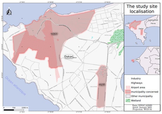
Figure 1.
Location of the Hlm and Yoff sampling sites.
Air masses could reach the sampling points undisturbed from all directions, and therefore the collected PM samples can be considered representative of the wider urban area. A low volume sampler from the University of GENT was used for sampling. The sampler is described in detail elsewhere [32]. Briefly, the sampler operates at a flow rate of 16 L min−1. It collects particulates that have an equivalent aerodynamic diameter (EAD) of less than 10 μm in separate “coarse” (2.5–10 μm EAD) and “fine” (<2.5 μm EAD) size fractions on two sequential 47 mm diameter filters. The discrimination against the >10 μm EAD particles is accomplished by a PM10 pre-impaction stage upstream of the stacked filter cassette. The air is drawn through the sampler by means of a diaphragm vacuum pump, which is enclosed in a special housing together with a needle valve, vacuum gauge, flow meter, volume meter, time switch (for interrupted sampling), and hour meter.
PM2.5 and PM2.5–10 were collected onto Nucleopore polycarbonate filters 47 mm diameter with 0.4 μm and 8 μm pore size, respectively [32]. After collection, the filters were kept in a desiccator to stabilize without hydration or contamination. The gravimetric quantification was performed with a Sartorius microbalance Secura and Quintix model 26 with an accuracy of 10−5 g. Filter weight was obtained from the average of three measurements when the variations were less than 0.5%.
During the years 2018–2019, a yearlong measurement campaign was performed to collect the PM2.5–10 and PM2.5 samples. The samples were collected twice per week; one sample during working days, and one during the weekend. This sampling protocol was selected to achieve the highest possible variation of source contributions, which is crucial for optimum performance of the source apportionment models. Several samples were collected throughout the period of 2018 and 2019, and 71 of each size fraction were selected to be analyzed by XRF. The selection was made to achieve maximum time coverage.
2.2. Elemental Analysis
The elemental composition of the samples was determined by Energy dispersive X-ray Fluorescence Spectroscopy (ED-XRF) using a commercially available system (Epsilon 5 by PANalytical, The Netherlands) [33]. Epsilon 5 is manufactured with optimized Cartesian-triaxial geometry and an extended K line excitation. A Ge X-ray detector is used to detect the characteristic X-rays emitted from the sample. The XRF system that was used is a secondary target system (ST-XRF). The system is equipped with nine secondary targets, and the operating conditions can be set for each target to achieve optimum analysis and performance. The total analysis time per sample was about 1.5 hour, and the operating conditions of the instrument are described in detail elsewhere [33].
Out of the 35 elements determined by the ED-XRF method, the ones used in the source apportionment analysis were Na, Mg, Al, Si, S, Cl, K, Ca, Ti, V, Cr, Mn, Fe, Co, Ni, Cu, Zn, Br, Sr, and Pb. For an element to be included in the source apportionment analysis, a threshold of at least 50% of points higher than the detection limit (DL) was set. The DLs were calculated following the approach described in [34]. The DLs were in the range of 10 to 24 ng m−3, and the uncertainties in the range of 1 to 16%. Since the uncertainties are a very important input in the PMF analysis, they were realistically estimated taking into account the individual uncertainties of every step of the analytical and sampling process [34].
2.3. Black Carbon Analysis
Black carbon (BC) or light absorbing carbon (LAC) is one of the most significant constituents of PM. A precise and accurate determination of both the concentration and source contribution of BC in air particulate samples can provide key information for both environmental management regulators and researchers. To measure (LAC) on the samples the Multi-wavelength absorption black carbon instrument (MABI) was used. The MABI (Figure 2), which is developed at ANSTO, measures the (Io) (measured light transmission through blank/unexposed filter) and (I) (measured light transmission through filter after particle sampling) values for seven different wavelengths which are used to determine the mass absorption coefficient and black carbon concentrations at each of these wavelengths. These wavelengths are 405, 465, 525, 639, 870, 940, and 1050 nm. MABI unit does not automatically calculate (BC) values in concentration units (μg m−3).
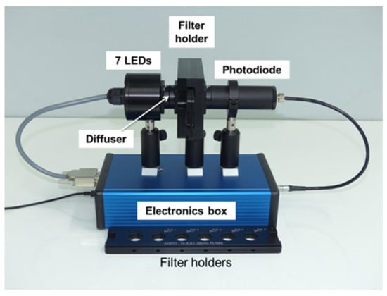
Figure 2.
ANSTO Multi-wavelength absorption black carbon instrument (MABI) Unit.
The first step for the calculation of BC values in concentration units (μg m−3) is the calculation babs (black carbon light absorption coefficient) using Equation (1). For that, it is necessary to know the exposed area of the filters (A) and sampled air volume (V).
- ϵ = Mass absorption coefficient in m2 g−1
- A = Filter collection area in cm2
- V = Volume of air sampled through the filter in m3
- Io’ Ro = Measured light transmission and reflection through blank (unexposed) filter
- I, R = Measured light transmission and reflection through filter after particle sampling.
The calculation of (BC) values in concentration units (μg m−3) is done by using Equation (3). The accuracy of these equations relies on the mass absorption coefficient (ε), which is a strong function of the size and density of the light absorbing particles. As black carbon can be emitted from a range of different sources with a range of different densities and sizes, ε is wavelength and density dependent. Ignoring this can result in an inaccurate estimation of black carbon concentrations depending on the dominant sources present. In the absence of any detailed information on aerosol state of mixing we use the default value 5.39 m2 g−1 at 870 nm for ε as provided by the manufacturer [34]. However, some indication on certain sources of PM is derived from the Angstrom exponent calculated from the MABI measurements on the 7 wavelengths. An indication for the Angstrom exponent is given when we plot the mass absorption coefficient for each wavelength (Figure 3). The value of −1267 indicated that part of the BC in our measurement sites originates from biomass burning [35].
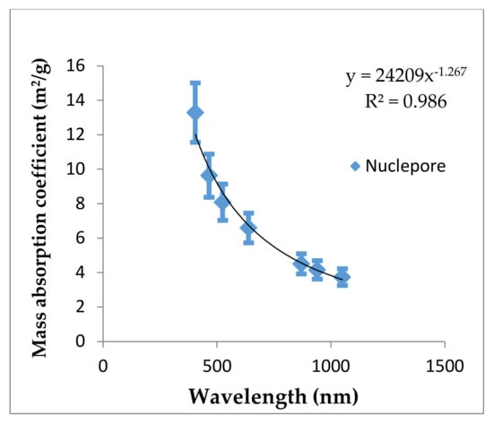
Figure 3.
Mass absorption coefficient vs wavelength for nucleopore filters.
2.4. PMF
The basic mass balance equation that is used by PMF can be written as
where X is the PM chemical composition matrix, G is the source contribution matrix, F the factor profile matrix, and E the residuals [36]. In PMF, G and F are constrained not to be negative (more accurately, only very slightly negative values are allowed). These constraints help the model achieve environmentally reasonable solutions, as it is impossible to have sources with negative contributions to PM mass.
The approach PMF follows to solve Equation (2), is to minimize the sum of the squares of the residuals scaled by the uncertainties of the data points. The task of PMF analysis can thus be described as to minimize Q, which is defined as:
where is the uncertainty of the jth species concentration in sample i, n is the number of samples [37].
As mentioned earlier, US-EPA PMF 5.0 version was used in this study. Twenty five variables were used as input in the model, and were namely PM, BC, Br, Rb, Sr, Ba, Pb, V, Cr, Mn, Fe, Co, Ni, Cu, Zn, Na, Mg, Al, Si, P, S, Cl, K, Ca, Ti. The variables with signal to noise (S/N) between 0.2 and 2 were defined as “Weak” in the model. PM mass was used as “total variable”. Species with S/N < 0.2 are assigned as “Bad” variables [38] and were excluded from the analysis. The elements defined as “Weak” variables were Na, P, V, Cr, Co, Ni, Br, Zn, Rb and Ba, while Mg was defined as “Bad” variable.
When the decrease in Q becomes small with an increasing number of factors, it is an indication that too many factors are being included in the fit [39]. In this study, a large number of factors (3 to 10) were tested and 4 were found to yield the optimum results. A < 5% difference was estimated between the Q robust and true values, as well as between the Q true and theoretical values. The total number of base runs was set to 100. All runs provided very similar results indicated by the very low difference between the scaled residuals of the different runs. To evaluate the rotational ambiguity of the solution, the uncertainty estimation tools provided by EPA PMF 5.0 were utilized. BS (bootstrap) analysis showed that the factors were stable, and were successfully reproduced at a level of at least 85%. displacement (DIS) and bootstrap-displacement (BS-DIS) analysis did not show any factor swaps for the lowest relevant Q change level. The correlation between modeled and true PM mass was estimated to be high (R2 = 0.75). All statistical indicators and uncertainty estimation tools show that the solution was well resolved, and the results had low uncertainty.
Because the number of species used for the source apportionment analysis represented a small fraction of PM mass, the contribution of the sources cannot be considered representative of the PM mass. Additionally, in such cases, the estimations have high relative uncertainty. For that reason, the source contributions are not reported.
2.5. Trajectory Analysis and Long-Range Transport
To assess the potential influence of long range transport events to PM concentrations, statistical trajectory methods (STMs) were used. The analysis was performed by using the OPENAIR software [40]. The HYSPLIT 4.0 model [41,42] developed by the NOAA (National Oceanic and Atmospheric Administration) was utilized to produce the back trajectory files. For the calculation of the trajectories, the GDAS meteorological database was used, and the calculations were done every 3 h for 120 h back, at a height level of 500 m above ground level (AGL). The STM that was used was the Potential Source Contribution Function (PSCF) [36,43]. The PSCF is estimated as:
where nij is the number of times that the trajectories passed through the cell (i, j) and mij is the number of times that a source concentration at the receptor was higher than a certain threshold (90th percentile) when the trajectories passed through the cell (i, j).
2.6. Air Quality Index (AQI)
AQI is used to identify the poor air quality zones in urban or industrial zones. The AQI of each pollutant is calculated by Equation (5):
where is the index for pollutant p
- is the truncated concentration of pollutant p
- is the concentration breakpoint that is greater than or equal to
- is the concentration breakpoint that is less than or equal to
- is the AQI value corresponding to
- is the AQI value corresponding to
3. Results
3.1. Concentration Level of Particulate Matter
The concentration levels of the collected PM size fractions in the two study sites are presented in Table 1.

Table 1.
Particulate matter (PM)2.5–10 and PM2.5 mass concentrations at Hlm and Yoff sites during the study period in μg m−3.
The mean values of PM2.5–10 concentrations at Hlm and Yoff are 246.16 and 240.03 μg m−3, respectively. The average PM2.5–10 concentration at the two sites is very similar, even though they have different characteristics (industrial and urban). This fact is an indication that anthropogenic emissions are not the dominant factor that affects PM mass in the area, which is most likely affected mainly by natural sources. The 24 hours limit value for the coarse particles in Senegal is 150 μg m−3 [44].
The average PM2.5 concentration at Hlm and Yoff is 280.58 and 302.73 μg m−3, respectively. PM2.5 concentration is higher in Yoff than in Hlm, indicating that urban activities in Dakar have a higher contribution in PM2.5 concentration levels than industrial activities. This might be related to the characteristics of the car fleet used in the city, which might lead to increased traffic-related emissions. Due to the extremely high PM2.5 concentrations, it can be assumed that dust also contributes to this fraction. Although dust particles are mostly related to coarse fractions of PM, it can also contribute significantly to PM2.5, as according to the size distributions, the lower tail of the coarse mode particles is found in PM2.5.
3.2. Elemental Concentration
The mean values and standard deviations of the elemental concentrations of the PM2.5 and PM2.5–10 samples in the two sites are presented in Table 2.
Table 2.
The average concentration and standard deviation (Stdev) of the elemental concentrations in sites during the studied period in μg m−3.
The elements that present the highest concentrations are Ca, Si, Cl, Al, Fe, Na, S, and K. All these elements originate mainly from natural sources, with the exception of K that can be a soil component but can also be emitted from biomass burning. Ca, Si, Al, and Fe are well-known soil components [45]. Na and Cl usually originate from sea salt, especially in coastal areas. S is found in the particulate phase mainly in the form of SO42−, which is formed by the oxidation of its precursor gas SO2. The elemental concentrations also indicate the importance of natural sources in the area, and especially of soil resuspension source.
3.3. Source Apportionment
Four factors with physical meaning were obtained using the EPA PMF model. The identified sources were namely mineral dust, sea salt/secondary sulfates, traffic emissions, and industrial emissions. The chemical composition of the sources is represented by the four factors from the PMF analysis presented in Figure 4.
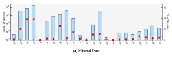
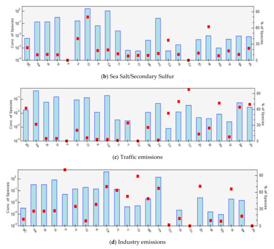
Figure 4.
PM sources profiles. The bars represent the normalized concentration of the species in the profile, and the squares show the contribution of the source to the average species concentration with (a) Mineral Dust, (b) Sea Salt/Secondary Sulfur, (c)Traffic and (d) Industry emissions.
The first factor has high loadings of Al, Si, and K that clearly indicates mineral dust as the origin source. This source might be somewhat mixed with biomass burning emissions, as K is a tracer of that source as well [46]. The low concentration of BC in the factor indicates that biomass burning contribution to the factor is low.
The second factor contains high concentration of Cl and Br corresponding to sea salt source. The factor also contains a very high percentage of S, which indicates that a factor is mixed with secondary sulfates. The fact that the two sources are mixed might be attributed to synchronous transportation from the sea or coastal region to the sampling point.
Factor 3 is identified as traffic emissions, and it contains a high concentration of BC, Cu, Ni, and Pb (>60%). In this factor we found also Rb and Ba. According to previous studies, Ni, Cu, Zn, Br, and Pb are related to exhaust traffic emissions [47]. Cu originates from break abrasion and Zn from the combustion of lubricating oil and tire wear [48].
Factor 4 is characterized by a high concentration (>50%) of P, Cr, Zn, Fe, Ti, Ca, and Mn that clearly indicates heavy industry, primary refinery, and/or coal mines, as well as the use of lubricant oils [49,50]. Around Hlm site, we found metallurgy industry, food factory, chemical industrial, and gas company.
Probably because of the very high dust load in the region (as indicated by the high concentrations of earth components/elements, >12 μg m−3 as sum of the elements in pure form), the presence of crustal elements/tracers is apparent in every factor. It has been shown in previous publications that if PM of certain origin have really high concentrations in a region (>50 μg m-3), their effect can be identified in other factors [51].
3.4. The Role of Long-Range Transport
The highest concentrations of coarse particulate matter (PM2.5–10) appear to be related to long-range transport from the Sahara desert. The highest concentrations of fine particulate matter (PM2.5) are transported from Mali. PSCF analysis (Figure 5) indicates source areas that affect the receptor during the days that the observed pollutant concentrations at the receptor are high. The fact that long-range transport affects the local PM concentrations, does not mean that the local contributions are low. PSCF analysis also indicates the strong influence of natural sources to PM levels in Dakar, and especially the influence of transported dust from the nearby arid regions. The fact that mineral dust particles affect the concentrations of PM in region, can also be confirmed by the high contributions of soil-related elements (Table 3).
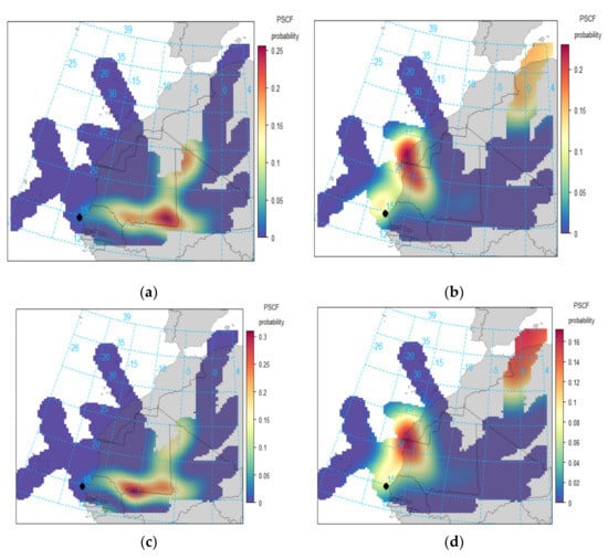
Figure 5.
Potential Source Contribution Functions (PSCFs) for the 85th percentile of (a) PM2.5 to Hlm, (b) PM2.5–10 to Hlm, (c) PM2.5 to Yoff and (d) PM2.5–10 to Yoff.
Table 3.
Breakpoint Concentration of air pollutants defined by U.S. EPA.
3.5. Air Quality Index (AQI)
The breakpoint concentrations have been defined by the EPA on the basis of National Ambient Air Quality Standards (NAAQS) as shown in Table 3 [52].
The highest individual pollutant index, Ip, represents the (AQI) of the location. The pollution level and status will be highlighted according to the (AQI) number, as shown in Table 3. The situation in an area can be classified from good to hazardous [53]. The conditions for ideal air quality was defined by [28].
Figure 6 and Figure 7 show the distribution of the air quality index (AQI) levels for the particulate matter PM2.5–10 and PM2.5 in Dakar. PM2.5–10 and PM2.5 represent in this study the “key pollutants”. The four major dynamic variables to interpreting the (AQI) time series were energy consumption structure, pollutant emissions, weather and topography of the city [54].
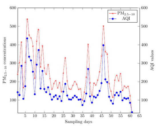
Figure 6.
Evolution of PM2.5–10 concentration and air quality index (AQI) values with time.
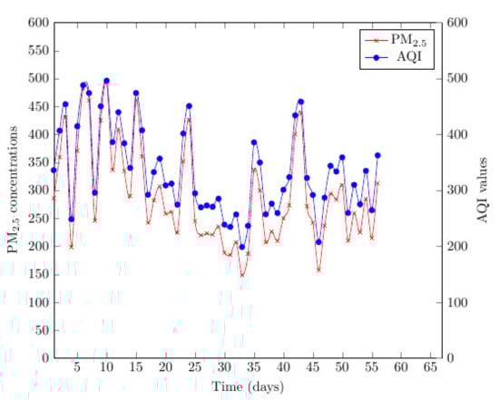
Figure 7.
Evolution of PM2.5 concentration and AQI values with time.
Figure 6 shows that (AQI) for the coarse particles ranges between 35 and 435. The figure includes the measurements conducted at both sites (Yoff and Hlm). The values of (AQI) are high in both areas. Furthermore Yoff site is close to the sea meaning that the air there is generally cleaner. The PM2.5–10 concentration is proportional to values (AQI) of 1.55. According to the findings of the study, the highest (AQI) value recorded in Hlm is approximately 488. This value is very high, even for an industrial area. Regarding Yoff the highest value of (AQI) was found to be approximately 497. We can conclude that Hlm and Yoff cities are severely polluted in PM2.5–10.
In Figure 7, the AQI for PM2.5 is presented. The (AQI) ranged between 199 and 497, which classifies the situation in the city from very unhealthy to hazardous. The (AQI) values for PM2.5 are more important than those of PM2.5–10 because the potential toxicology impact PM2.5 is higher. The highest values of (AQI) are approximately 497 and 488, in Yoff and Hlm, respectively. In contrast to what was found for the coarse particles, the (AQI) for PM2.5 is higher in the urban zone.
4. Conclusions
This study took place in the capital city of Senegal, Dakar; a coastal area of 5 million inhabitants. The measurement campaign took place during the years 2018 and 2019. PM2.5–10 and PM2.5 samples were collected twice per week (one on a working day and one during weekend). The average concentration of PM2.5–10 at Hlm and Yoff were found equal to 246.16 and 240.03 μg m−3, respectively, while the average concentration of PM2.5 was 280.58 and 302.73 μg m−3, respectively. The concentration of the coarse particles was higher in Hlm, whereas the fine particles are more important in Yoff site. The elemental composition of the PM samples was determined using XRF. The elements that present the highest concentrations are Ca, Si, Cl, Al, Fe, Na, S, and K. All these elements originate mainly from natural sources, with the exception of K that can be a soil component but can also be emitted from biomass burning. According to PSCF, the high PM2.5 and PM2.5–10 concentration levels were related to long-range transportation events from Mali and Sahara desert, respectively. The sources of PM2.5–10 and PM2.5 were identified using EPA PMF 5.0. Four PM sources were identified: industrial emissions, mineral dust, traffic emissions, and sea salt/secondary sulfates. (AQI) for the coarse particles ranged between 35 and 435, and based on those findings, it can be said that Hlm and Yoff cities are severely polluted in PM2.5–10. (AQI) for PM2.5 ranged between 199 and 497, which classifies the situation in the city from very unhealthy to hazardous.
This study is the first study that investigates the sources of PM2.5–10 and PM2.5 in Dakar. The information summarized are important as it can provide information to the people and the government of Senegal about the particulate related pollution in the area. It must be notted here that the extremely high particulate levels found in Dakar are mainly due to mineral particles (desert dust and locally resuspended mineral particles). It is not easy to aseess the pollution levels based only on an AQI calculation that takes into account the concentrations of suspended particles, even though the concentrations of fine particles are indeed very high. The relatively limited available data concerning the chemical composition of PM (and the lack of data about gas concentrations) do not allow to conclude definitively about the seriousness of the air pollution in Dakar, since as stated before the estimates presented in this study are based mainly on the overall concentration, and not on PM chemical composition. Further studies will be necessary to arrive at a more realistic state of air quality in this city, that include the measurement of additional PM chemical components and better quantification of source contributions.
Author Contributions
Conceptualization, A.T. and M.I.M.; methodology, A.T. and M.K.; validation, M.K., A.T., and M.I.M.; formal analysis, M.K., M.I.M., and V.V.; writing—original draft preparation, A.T. and M.K.; writing—review and editing, A.T. and M.I.M.; supervision, A.T.; Administrative issue, A.S.N., A.W., and K.E. All authors have read and agreed to the published version of the manuscript.
Funding
This research was funded by the International Atomic Energy Agency in Vienna under the framework of the Regional technical project RAF7016.
Institutional Review Board Statement
Not applicable.
Informed Consent Statement
Not applicable.
Data Availability Statement
Not applicable.
Acknowledgments
We are very grateful to Roman Padilla Alvarez for his support during the entire duration of the project, the sampling protocol and advices.
Conflicts of Interest
The authors declare no conflict of interest.
References
- Elichegaray, C. Département Air à l’Agence de l’environnement et de la maîtrise de l’énergie (ADEME). Pollut. Atmosphérique 2001, 8. [Google Scholar]
- Li, W.; Bai, Z.; Liu, A.; Chen, J.; Chen, l. Characteristics for major PM2.5 components during winter in Tianjin, China. Aerosol Air Qual. Res. 2009, 9, 105–119. [Google Scholar] [CrossRef]
- Katsouyanni, K.; Touloumi, G.; Samoli, E.; Gryparis, A.; Le Tertre, A.; Monopolis, Y.; Rossi, G.; Zmirou, D.; Ballester, F.; Boumghar, A.; et al. Confounding and effect modification in the short-term effects of ambient particles on total mortality: Results from 29 European cities within the APHEA2 Project. Epidemiology 2001, 12, 521–531. [Google Scholar] [CrossRef] [PubMed]
- Liu, Y.; Daum, P.H. Anthropogenic aerosols: Indirect warming effect from dispersion forcing. Nature 2002, 419, 580–581. [Google Scholar] [CrossRef]
- Pandolfi, M.; Alastuey, A.; Pérez, N.; Reche, C.; Castro, I.; Shatalov, V.; Querol, X. Trends analysis of PM source contributions and chemical tracers in NE Spain during 2004–2014: A multi-exponential approach. Atmospheric Chem. Phys. 2016, 16, 11787–11805. [Google Scholar] [CrossRef]
- Manousakas, M.; Popovicheva, O.; Evangeliou, N.; Diapouli, E.; Sitnikov, N.; Shonija, N.; Eleftheriadis, K. Aerosol carbonaceous, elemental and ionic composition variability and origin at the Siberian High Arctic, Cape Baranova. Tellus B Chem. Phys. Meteorol. 2020, 72, 1–14. [Google Scholar] [CrossRef]
- Guaita, R.; Pichiule, M.; Mate, T.; Linares, C.; Diaz, J. Short-term impact of particulate matter (PM2.5) on respiratory mortality in Madrid. Int. J. Environ. Health Res. 2011, 21, 260–274. [Google Scholar] [CrossRef]
- Halonen, J.I.; Lanki, T.; Tuomi, T.Y.; Tiittanen, P.; Kulmala, M.; Pekkanen, J. Particulate air pollution and acute cardiorespiratory hospital admissions and mortality among the elderly. Epidemiology 2009, 20, 143–153. [Google Scholar] [CrossRef]
- Perez, L.; Tobías, A.; Querol, X.; Pey, J.; Alastuey, A. Saharan dust, particulate matter and cause-specific mortality: A case-crossover study in Barcelona (Spain). Environ. Int. 2012, 48, 150–155. [Google Scholar] [CrossRef]
- Samoli, E.; Peng, R.; Ramsay, T.; Pipikou, M.; Touloumi, G.; Dominici, F.; Burnett, R.; Cohen, A.; Krewski, D.; Samet, J.; et al. Acute effects of ambient particulate matter on mortality in Europe and North America: Results from the APHENA Study. Environ. Health Perspect. 2008, 116, 1480–1486. [Google Scholar] [CrossRef]
- Cesari, D.; Donateo, A.; Conte, M.; Contini, D. Inter-comparison of source apportionment of PM10 using PMF and CMB in three sites nearby an industrial area in central Italy. Atmos. Res. 2016, 182, 282–293. [Google Scholar] [CrossRef]
- Freer-Smith, P.H.; Beckett, K.P.; Taylor, G. Deposition velocities to Sorbus aria, Acer campestre, Populus deltoides, Pinus nigra and Cupressocyparis leylandii for coarse, fine and ultra-fine particles in the urban environment. Environ. Pollut. 2005, 133, 157–167. [Google Scholar] [CrossRef] [PubMed]
- Cheung, K.; Daher, N.; Kam, W.; Shafer, M.M.; Ning, Z.; Schauer, J.J.; Sioutas, C. Spatial and temporal variation of chemical composition and mass closure of ambient coarse particulate matter (PM10–2.5) in the Los Angeles area. Atmos Environ. 2011, 45, 2651–2662. [Google Scholar]
- Psanis, C.; Triantafyllou, E.; Giamarelou, M.; Manousakas, M.; Eleftheriadis, K.; Biskos, G. Particulate matter pollution from aviation-related activity at a small airport of the Aegean Sea Insular Region. Sci. Total Environ. 2017, 596–597, 187–193. [Google Scholar] [CrossRef] [PubMed]
- Dall’Osto, M.; Querol, X.; Amato, F.; Karanasiou, A.; Lucarelli, F.; Nava, S.; Calzolai, G.; Chiari, M. Hourly elemental concentrations in PM2.5 aerosols sampled simultaneously at urban background and road site during SAPUSS—Diurnal variations and PMF receptor modelling. Atmos. Chem. Phys. 2013, 13, 4375–4392. [Google Scholar] [CrossRef]
- Shaka’, H.; Saliba, N.A. Concentration measurements and chemical composition of PM10–2.5 and PM2.5 at a coastal site in Beirut, Lebanon. Atmos. Environ. 2004, 38, 523–531. [Google Scholar] [CrossRef]
- Maenhaut, W.; Francois, F.; Cafmeyer, J. The Gent Stacked Filter Unit (Sfuj Sampler for the Collection of Atmospheric Aerosols in Two Size Fractions: Description and Instructions for Installation and Use); Report N°. NAHRES-19; IAEA: Vienna, Austria, 1993; pp. 249–263. [Google Scholar]
- Chow, J.C. Critical review: Measurement methods to determine compliance with ambient air quality standards for suspended particles. J. Air Waste Manag. Assoc. 1995, 45, 320–382. [Google Scholar] [CrossRef]
- Wilson, W.E.; Chow, J.C.; Claiborn, C.; Fusheng, W.; Engelbrecht, J.; Watson, J.G. Monitoring of particulate matter outdoors. Chemosphere 2002, 49, 1009–1043. [Google Scholar] [CrossRef]
- Van Griekan, R.; Markowicz, A.; Veny, P. Current trends in the literature on x-ray emission spectrometry. X-ray Spectr. 1991, 20, 271–276. [Google Scholar]
- Dzubay, T.G.; Hines, L.E.; Stevens, R.K. Particle bounce errors in cascade impactors. Atmos. Environ. 1976, 10, 229–234. [Google Scholar] [CrossRef]
- Viana, M.; Kuhlbusch, T.A.J.; Querol, X.; Alastuey, A.; Harrison, R.M.; Hopke, P.K.; Winiwarter, W.; Vallius, M.; Szidat, S.; Prévôt, A.S.H.; et al. Source apportionment of particulate matter in Europe: A review of methods and results. J. Aerosol Sci. 2008, 39, 827–849. [Google Scholar] [CrossRef]
- Belis, C.A.; Pernigotti, D.; Pirovano, G.; Favez, O.; Jaffrezo, J.L.; Kuenen, J.; van Der Gon, H.G.; Reizer, M.; Riffault, V.; Alleman, L.Y.; et al. Evaluation of receptor and chemical transport models for PM10 source apportionment. Atmos. Environ. X 2020, 5, 100053. [Google Scholar] [CrossRef]
- Manousakas, M.; Diapouli, E.; Belis, C.A.; Vasilatou, V.; Gini, M.; Lucarelli, F.; Querol, X.; Eleftheriadis, K. Quantitative assessment of the variability in chemical profiles from source apportionment analysis of PM10 and PM2.5 at different sites within a large metropolitan area. Environ. Res. 2021, 192, 110257. [Google Scholar] [CrossRef] [PubMed]
- Paatero, P.; Tapper, U. Positive matrix factorization: A non-negative factor model with optimal utilization of error estimates of data values. Environmetrics 1994, 5, 111–126. [Google Scholar] [CrossRef]
- Johnson, T.M.; Guttikunda, S.; Wells, G.J.; Artaxo, P.; Bond, T.C.; Russell, A.G.; Watson, J.G.; West, J. Tools for Improving Air Quality Management, A Review of Top-Down Source Apportionment Techniques and Their Application in Developing Countries; ESMAP: Washington, DC, USA, 2011; p. 220. [Google Scholar]
- Amato, F.; Alastuey, A.; Karanasiou, A.; Lucarelli, F.; Nava, S.; Calzolai, G.; Severi, M.; Becagli, S.; Gianelle, V.L.; Colombi, C.; et al. AIRUSE-LIFEC: A harmonized PM speciation and source apportionment in five southern European cities. Atmos. Chem. Phys. 2016, 16, 3289–3309. [Google Scholar]
- Kanchan, K.; Gorail, A.K.; Pramila, G. A Review on Air Quality Indexing System. Asian J. Atmos. Environ. 2015, 9, 101–113. [Google Scholar] [CrossRef]
- Available online: http://www.denv.gouv.sn/index.php/air-et-climat/centre-de-gestion-de-la-qualite-de-l-air-cgqa/pollution (accessed on 7 August 2019).
- Rivellini, L.H.; Chiapello, I.; Tison, E.; Fourmentin, M.; Féron, A.; Diallo, A.; N’Diaye, T.; Goloub, P.; Canonaco, F.; Prévôt, A.S.; et al. Chemical characterization and source apportionment of submicron aerosols measured in Senegal during the 2015 SHADOW campaign. Atmos. Chem. Phys. 2017, 17, 10291–10314. [Google Scholar] [CrossRef]
- Ba, A.N.; Verdin, A.; Cazier, F.; Garcon, G.; Thomas, J.; Cabral, M.; Dewaele, D.; Genevray, P.; Garat, A.; Allorge, D.; et al. Individual exposure level following indoor and outdoor air pollution exposure in Dakar (Senegal). Environ. Pollut. 2019, 248, 397–407. [Google Scholar]
- Hopke, P.K.; Xie, Y.; Raunemaa, T.; Biegalski, S.; Landsberger, S.; Maenhaut, W.; Artaxo, P.; Cohen, D. Characterization of the Gent Stacked Filter Unit PM10 Sampler. Aerosol Sci. Technol. 1997, 27, 726–735. [Google Scholar] [CrossRef]
- Manousakas, M.; Diapouli, E.; Papaefthymiou, H.; Kantarelou, V.; Zarkadas, C.; Kalogridis, A.-C.; Karydas, A.G.; Eleftheriadis, K. XRF characterization and source apportionment of PM10 samples collected in a coastal city. X-ray Spectr. 2018, 47, 190–200. [Google Scholar]
- Cohen, D.D. Summary of Light Absorbing Carbon and Visibility Measurements and Terms. In ANSTO External Report ER-790; ANSTO: Sydney, Australia, 2020; ISBN 1 921268 32 8. [Google Scholar]
- Diapouli, E.; Kalogridis, A.; Markantonaki, C.; Vratolis, S.; Fetfatzis, P.; Colombi, C.; Eleftheriadis, K. Annual variability of black carbon concentrations originating from biomass and fossil fuel combustion for the suburban aerosol in Athens, Greece. Atmosphere 2017, 8, 234. [Google Scholar] [CrossRef]
- Manousakas, M.I.; Florou, K.; Pandis, S.N. Source Apportionment of Fine Organic and Inorganic Atmospheric Aerosol in an Urban Background Area in Greece. Atmosphere 2020, 11, 330. [Google Scholar] [CrossRef]
- Chueinta, W.; Hopke, P.K.; Paatero, P. Investigation of sources of atmospheric aerosol at urban and suburban residential areas in Thailand by positive matrix factorization. Atmos. Environ. 2000, 34, 3319–3329. [Google Scholar] [CrossRef]
- Paatero, P.; Hopke, P.K. Discarding or down weighting high-noise variables in factor analytic models. Anal. Chim. Acta. 2003, 490, 277–289. [Google Scholar] [CrossRef]
- Xie, Y.L.; Hopke, P.K.; Paatero, P.; Barrie, L.A.; Li, S.-M. Identification of source nature and seasonal variations of Arctic aerosol by positive matrix factorization. J. Atmos. Sci. 1999, 56, 249–260. [Google Scholar] [CrossRef]
- Carslaw, D.C.; Ropkins, K. Openair—An R package for air quality data analysis. Environ. Model. Softw. 2012, 27, 52–61. [Google Scholar] [CrossRef]
- Stein, A.F.; Draxler, R.R.; Rolph, G.D.; Stunder, B.J.B.; Cohen, M.D.; Ngan, F. Noaa’s hysplit atmospheric transport and dispersion modeling system. Bull. Am. Meteorol. Soc. 2015, 96, 2059–2077. [Google Scholar] [CrossRef]
- Rolph, G.; Stein, A.; Stunder, B. Real-time environmental applications and display system: READY. Environ. Model. Softw. 2017, 95, 210–228. [Google Scholar] [CrossRef]
- Stohl, A. Trajectory statistics—A new method to establish source-receptor relationships of air pollutants and its application to the transport of particulate sulfate in Europe. Atmos. Environ. 1996, 30, 579–587. [Google Scholar] [CrossRef]
- Senegalese Norm. 2018; ISO NS 05-062.
- Vasilatou, V.; Manousakas, M.; Gini, M.; Diapouli, E.; Scoullos, M.; Eleftheriadis, K. Long Term Flux of Saharan Dust to the Aegean Sea around the Attica Region, Greece. Front. Mar. Sci. 2017, 4, 42. [Google Scholar] [CrossRef]
- Diapouli, E.; Popovicheva, O.; Kistler, M.; Vratolis, S.; Persiantseva, N.; Timofeev, M.; Kasper-Giebl, A.; Eleftheriadis, K. Physicochemical characterization of aged biomass burning aerosol after long-range transport to Greece from large scale wildfires in Russia and surrounding regions, Summer 2010. Atmos. Environ. 2014, 96, 393–404. [Google Scholar] [CrossRef]
- Zhang, N.; Cao, J.; Ho, K.; He, Y. Chemical characterization of aerosol collected at Mt. Yulong in wintertime on the southeastern Tibetan Plateau. Atmos. Res. 2012, 107, 76–85. [Google Scholar] [CrossRef]
- Sternbeck, J.; Sjodin, A.; Andreasson, K. Metal emissions from road traffic and the influence of resuspension—results from two tunnel studies. Atmos. Environ. 2002, 36, 4735. [Google Scholar] [CrossRef]
- Manousakas, M.; Papaefthymiou, H.; Diapouli, E.; Migliori, A.; Karydas, A.G.; Bogdanovic-Radovic, I.; Eleftheriadis, K. Assessment of PM2.5 sources and their corresponding level of uncertainty in a coastal urban area using EPA PMF 5.0 enhanced diagnostics. Sci. Total Environ. 2017, 574, 155–164. [Google Scholar] [CrossRef]
- Pateraki, S.; Manousakas, M.; Bairachtari, K.; Kantarelou, V.; Eleftheriadis, K.; Vasilakos, C.; Assimakopoulos, V.D.; Maggos, T. The traffic signature on the vertical PM profile: Environmental and health risks within an urban roadside environment. Sci. Total Environ. 2019, 646, 448–459. [Google Scholar] [CrossRef]
- Gunchin, G.; Manousakas, M.; Osan, J.; Karydas, A.G.; Eleftheriadis, K.; Lodoysamba, S.; Shagjjamba, D.; Migliori, A.; Padilla-Alvarez, R.; Streli, C.; et al. Three-year Long Source Apportionment Study of Airborne Particles in Ulaanbaatar Using X-ray Fluorescence and Positive Matrix Factorization. Aerosol Air Qual. Res. 2019, 19, 1056–1067. [Google Scholar] [CrossRef]
- Mintz, D. Technical Assistance Document for the Reporting of Daily Air Quality—The Air Quality Index (AQI); US-EPA: Washington, DC, USA, 2018; 454/B-18-007. [Google Scholar]
- Wang, L.; Zhang, P.; Tan, S.; Zhao, X.; Cheng, D.; Wei, W.; Su, J.; Pan, X. Assessment of urban air quality in China using air pollution indices (APIs). J. Air Waste Manag. 2013, 63, 170–178. [Google Scholar] [CrossRef]
- Yu, B.; Huang, C.M.; Liu, Z.H.; Wang, H.P.; Wang, L.L. A chaotic analysis on air pollution index change over past 10 years in Lanzhou, northwest China. Stochastic Environ. Res. 2011, 25, 643–653. [Google Scholar] [CrossRef]


Publisher’s Note: MDPI stays neutral with regard to jurisdictional claims in published maps and institutional affiliations. |
© 2021 by the authors. Licensee MDPI, Basel, Switzerland. This article is an open access article distributed under the terms and conditions of the Creative Commons Attribution (CC BY) license (http://creativecommons.org/licenses/by/4.0/).