Probabilistic Forecasting of the 500 hPa Geopotential Height over the Northern Hemisphere Using TIGGE Multi-model Ensemble Forecasts

Abstract

Bayesian model averaging (BMA) and ensemble model output statistics (EMOS) were used to improve the prediction skill of the 500 hPa geopotential height field over the northern hemisphere with lead times of 1–7 days based on ensemble forecasts from the European Centre for Medium-Range Weather Forecasts (ECMWF), National Centers for Environmental Prediction (NCEP), and UK Met Office (UKMO) ensemble prediction systems. The performance of BMA and EMOS were compared with each other and with the raw ensembles and climatological forecasts from the perspective of both deterministic and probabilistic forecasting. The results show that the deterministic forecasts of the 500 hPa geopotential height distribution obtained from BMA and EMOS are more similar to the observed distribution than the raw ensembles, especially for the prediction of the western Pacific subtropical high. BMA and EMOS provide a better calibrated and sharper probability density function than the raw ensembles. They are also superior to the raw ensembles and climatological forecasts according to the Brier score and the Brier skill score. Comparisons between BMA and EMOS show that EMOS performs slightly better for lead times of 1–4 days, whereas BMA performs better for longer lead times. In general, BMA and EMOS both improve the prediction skill of the 500 hPa geopotential height field.

1. Introduction

Numerical weather prediction is an important technique in modern weather forecasting in which the basic equations of atmospheric motion are solved numerically to predict the future state of the atmosphere given the initial and boundary conditions [1,2]. However, chaos theory shows that even small perturbations in the initial conditions will lead to very different forecasts [3,4]. The prediction skill of a single deterministic forecast is limited by the uncertainties associated with the models and the initial conditions [5,6]. It is therefore necessary to use probabilistic forecasting rather than deterministic forecasting to provide a better numerical weather prediction service.

Probabilistic weather prediction describes the probability of the occurrence of future weather events as a percentage [7]. The forecast information (i.e., the uncertainty and probability) provided by probabilistic weather prediction is important in decision-making and can help to predict extreme weather events [8,9,10]. Probabilistic forecasting gradually became operational in many countries and regions from about 1960—for example, the Meteorological Development Laboratory of the US National Weather Service has tested and operationally run the model output statistics forecast equation as a tool for weather forecasting since the 1990s.

Ensemble forecasting is a key technique used for conceptual transition from a single deterministic forecast to a probabilistic forecast [11,12,13]. Ensemble forecasting aims to quantitatively describe the uncertainty of the forecast and to provide a more reliable probability density function (PDF) rather than a better deterministic forecast [14,15]. However, ensemble forecasts are usually biased and under-dispersed as a result of the imperfect ensemble prediction system (EPS) and the limited initial perturbation schemes [16,17]. Several statistical post-processing methods have therefore been proposed and applied to reduce systematic errors and forecast uncertainties [18,19,20,21,22,23,24,25,26,27].

Ensemble model output statistics (EMOS) [28,29,30] and Bayesian model averaging (BMA) [31,32,33] are the two most popular and effective post-processing methods for the correction of bias in ensemble forecasting and produce probabilistic forecasts. The BMA method combines predictive PDFs from different EPSs by weighted averages. The weights are equal to the posterior probabilities of the EPSs and reflect their relative performance during the training period. Contributing EPSs with a better performance over the training period will be assigned a larger weight and will thus contribute more to the BMA predictive PDF. The EMOS method generates a single parametric PDF using the raw ensemble forecasts directly rather than combining their kernels or PDFs, which need to be computed separately in BMA. The predictive parameters in EMOS are estimated using multiple regression equations with the raw ensemble forecasts and the corresponding verifications over a training period. Both BMA and EMOS have been applied to several different weather quantities (i.e., temperature, wind, and precipitation) and have been shown to improve prediction skills relative to the raw ensembles [34,35,36,37,38,39,40,41,42,43,44,45,46,47].

Few studies have applied BMA and EMOS to the geopotential height for probabilistic forecasting. The geopotential height field reflects the state of the atmosphere circulation and has an important influence on the regional and hemispheric climate. It is also important in short- and medium-range weather forecasts [48,49,50,51,52,53]. An improvement in forecasting of the 500 hPa geopotential height field will help forecasters to better understand large-scale atmospheric circulation patterns and give more accurate predictions of the weather. We therefore used these two ensemble-based statistical post-processing methods for bias correction and probabilistic forecasting of the 500 hPa geopotential height in the northern hemisphere and compared their performance.

The rest of this paper is organized as follows. Section 2 describes the datasets and the BMA and EMOS methods and introduces the verification methods. Section 3 compares the raw ensembles and forecasts obtained from the BMA and EMOS prediction models and our summary and conclusions are presented in Section 4.

2. Data and Methods

2.1. Data

We used multi-member 500 hPa geopotential height forecasts produced by the European Centre for Medium-Range Weather Forecasts (ECMWF), the National Centers for Environmental Prediction (NCEP) and the UK Met Office (UKMO) EPSs at a horizontal resolution of 2.5° × 2.5°. The forecasts were initialized daily at 1200 UTC for lead times of 1–7 days using the TIGGE datasets (

Table 1. Comparison of the three single-center ensemble prediction systems used in this study.

Center	Domain	Model Resolution	Ensemble Members (Perturbed)	Lead Time (Days)
ECMWF	Europe	T399L62/T255L62	50	15
NCEP	USA	T216L28	20	16
UKMO	UK	1.5° × 1.875°	23	15

). The TIGGE datasets are a key component of THORPEX and have collected ensemble forecast data from 10 global model prediction centers since 2006. We analyzed the data for the northern hemisphere for a one-year period from 1 January to 31 December 2013. The ECMWF ERA5 reanalysis dataset for the 500 hPa geopotential height products at 1200 UTC was used as the verification dataset.

2.2. Bayesian Model Averaging

The BMA method was first applied to the ensemble forecasting of surface pressure and temperature by Raftery et al. [31]. Following their research, the BMA predictive PDF of a weather quantity y is a weighted average of the individual PDFs centered on the bias-corrected forecasts corresponding to the members of the ensemble. The weights reflect the relative performance of the ensemble members during a given training period. Raftery et al. [31] suggested that temperature and sea-level pressure can be fitted reasonably well by a normal distribution. The BMA predictive PDF is then given by

$$P\left(y|f_1,\dots ,f_K\right)={\displaystyle \sum }_{k=1}^K{\omega }_k{g}_k(y|f_k)$$

(1)

where $f_k$ is the forecast of the kth model, $g_k(\mathrm{y}|f_k)$ is the conditional normal PDF with a mean of $(a_k+b_k{f}_k$) and a standard deviation $\sigma$. ${\omega }_k$ is the weight corresponding to the performance of the kth model in the given training period. A simple linear regression is used to estimate the BMA parameters $a_k$ and $b_k \left(k = 1, 2, \dots , K\right)$; ${\omega }_k$ and $\sigma$ are estimated by a maximum likelihood method [31,54].

The BMA parameters are estimated during a training period. A sliding training period has been proved to be better than a fixed period [55]. We therefore retrained the BMA prediction model on each grid point in the study area every day throughout the forecast period using a training sample period of N previous days. The performance of different BMA prediction models using different lengths of training period showed that the previous 45 days before the forecast period was the optimum length of the training period (not shown).

2.3. Ensemble Model Output Statistics

The EMOS predictive PDF of a weather quantity y is single parametric where the parameters are obtained from the ensemble members of the contributing EPSs. Following Gneiting et al. [28], the EMOS normal predictive distribution is defined as:

$$P\left(y|f_1,\dots ,f_K\right)~N\left(a+b_1{f}_1+\dots +b_K{f}_K,c+d{S}^2\right)$$

(2)

with $f_1,\dots , f_K$, for the K-member of an individually distinguishable forecast at a geopotential height of 500 hPa. a and $b_1,\dots , b_K$ are the regression coefficients. $S^2$ is the ensemble variance with non-negative coefficients c and d. We estimated the EMOS coefficients by minimizing the continuous ranked probability score (CRPS) during the training period. Our EMOS experiments were partially implemented in the ensembleMOS packages of R.

2.4. Verification Methods

We used the root mean square error (RMSE) to evaluate the deterministic forecast of the raw ensemble, BMA and EMOS forecasts. The CRPS, Brier score (BS), and Brier skill score (BSS) were adopted to assess the probabilistic forecasts.

2.4.1. Root Mean Square Error

The RMSE is the square root of the average of the squared differences between the forecasts and observations:

$$RMSE=\sqrt{\frac{1}{N}{\displaystyle \sum }_{i=1}^N{(y_i-o_i)}^2 }$$

(3)

where N is the total number of grid points and $y_i$ and $o_i$ are the model forecast and observed value of the ith grid sample, respectively. The RMSE is negatively oriented, which means that a smaller value indicates a better prediction skill.

2.4.2. Continuous Ranked Probability Score

The CRPS is a measure of the integrated squared difference between the cumulative distribution function of the forecasts and the corresponding cumulative distribution function of the observations:

$$CRPS= \frac{1}{N}{\displaystyle \sum }_{i=1}^N{\displaystyle \int }{[f(y_i)-H\left(y_i-o_i\right)]}^{2}dx$$

(4)

$$H\left(y_i-o_i\right)=\{\begin{array}{c}1, y_i\ge o_i\\ 0, y_i<o_i\end{array}$$

(5)

where $f\left(y_i\right)$ is the forecast cumulative distribution function (CDF) at model forecast $y_i$ and $o_i$ is the corresponding observed value. $H\left(y_i-o_i\right)$ is the Heaviside function and is equal to 1 when $y_i\ge o_i$, otherwise it has a value of 0. The CRPS is also negatively oriented and 0 indicates a perfect score.

2.4.3. Brier Score and Brier Skill Score

The BS is the mean square error of probabilistic two-category forecasts [56]:

$$BS = \frac{1}{n}{{\displaystyle \sum }}_{i=1}^n{(f_i-O_i)}^2$$

(6)

where n is the number of forecast–event pairs,$f_i$ is the forecast probability and $O_i$ is the observation, which is either 0 (no occurrence) or 1 (occurrence). The BS ranges from 0 to 1 and is 0 for perfect forecasts.

The BSS is a skill score based on the values of the BS to assess the relative improvement of the forecast over the reference forecast [57].

$$BSS=1-\frac{BS (forecast)}{BS \left(reference\right)}$$

(7)

We used the climatological forecast as the reference forecast. The climatological probability of the sample was determined for each month and each grid point to consider the differences between the frequency of the climatological event in different regions within the northern hemisphere [58]. The forecast was considered to be perfect when BSS = 1. BSS > 0 meant that there was an improvement compared to the reference (climatological) forecast.

3. Results

3.1. Deterministic Forecasts

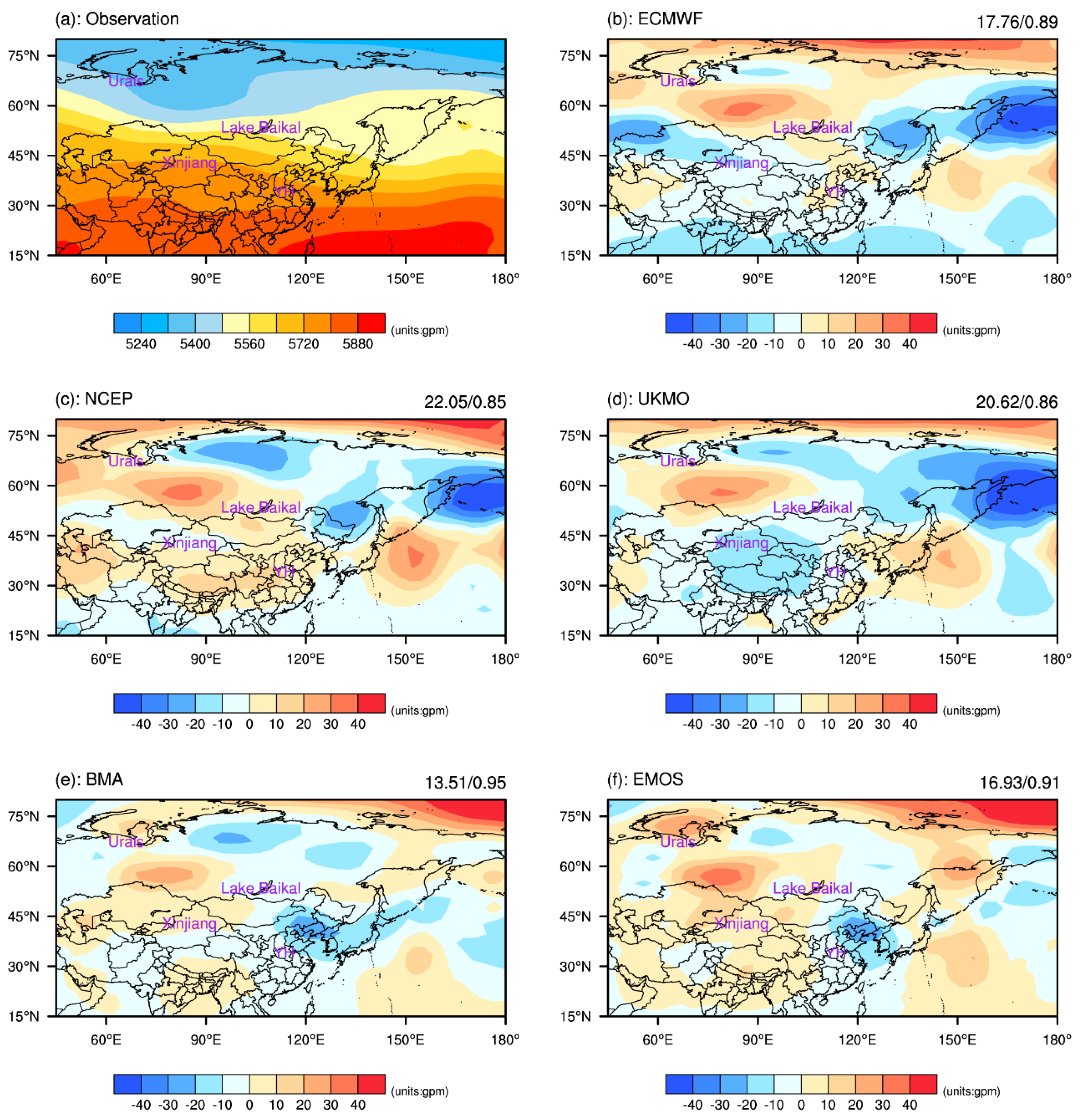
We selected two extreme events to investigate the performance of the deterministic forecasts by raw ensembles and two statistical post-processing methods (BMA and EMOS). The first extreme event was the persistent severe rainstorms that occurred in South China from late March 2013. Continuous extreme precipitation processes mainly occurred during the periods 26 March–11 April and 23 April–30 May. The intensity of precipitation was significantly stronger in the second period than in the first period and was affected by the west Pacific subtropical high (WPSH, the area surrounded by the 5880 gpm line on the 500hPa geopotential height) and the South China Sea monsoon. The WPSH covered a larger area and was more intense than the climatological average and the location of the WPSH ridge was further south [59,60]. The observed distribution of the 500 hPa geopotential height showed two relatively stable ridges of high pressure located to the west of the Ural Mountains and east of Lake Baikal, respectively (Figure 1). Northeast China, North China, and the Yellow and Huaihe river basins were therefore mainly controlled by high-pressure ridges, whereas the area from Xinjiang to the west of Lake Baikal was a low-pressure trough in the 500 hPa geopotential height field. The deterministic forecasts of the ECMWF, NCEP, and UKMO EPSs were similar. They all predicted higher values of 500 hPa geopotential height between the Urals and Lake Baikal, and lower values in the east of Russia compared to the observations. The ECMWF and UKMO EPSs had under-forecasted the geopotential height over China, while NCEP EPS had slightly larger predictions. For WSPH area in the northern hemisphere shown in the observations, the raw ensemble predictions with the lead times of 7 days were not strong enough. The difference between the observations and deterministic forecasts of BMA and EMOS were smaller in comparison of the raw ensembles, with the smallest RMSE and highest ACC values. The location and area predictions of the WPSH using the BMA and EMOS methods were fairly similar to the observations, even with lead times of 7 days.

The second extreme event was the heatwaves that occurred in the summer of 2013. The average number of heatwave days (daily maximum temperature > 35 °C) in this summer was 31 days, the highest number since 1951 [61]. The temperature in South China was abnormally high and there were many extreme high temperature events. One of the main reasons for this heatwave event was that the WPSH was significantly further north than normal. The WPSH frequently strengthens and expands westward into inland areas, so that most of South China is controlled by the western side of the subtropical high [62]. This strengthened WSPH causes a stronger downward movement of air, weaker convection, and less precipitation in these regions, leading to extreme high temperature events in South China. The raw ensembles predicted higher values in northern Russia and lower values in western Pacific. The BMA and EMOS deterministic forecasts of BMA and EMOS were similar to the observations, whereas the ECMWF, NCEP, and UKMO EPSs predicted a weaker WPSH than the observations (Figure 2).

3.2. Probabilistic Forecasts

Figure 3 shows the predictive PDFs obtained from the BMA, EMOS and raw ensemble forecasts for a certain grid point. The raw ensemble PDFs tended to spread the distribution, whereas the BMA and EMOS predictive PDFs were sharper and more concentrated than the raw ensembles. The EMOS PDF was sharper than the BMA PDF.

Probabilistic forecasting maximizes the sharpness of the predictive PDF through calibration [31,63]. We therefore evaluated the calibration using the verification rank histogram [64,65] for the raw ensemble forecasts and the probability integral transform (PIT) histogram [18] for the BMA and EMOS forecast distributions. A straight and uniform distribution characterizes an “ideal” EPS. The verification rank histograms for the ECMWF EPS showed a U-shaped distribution (Figure 4). These uneven distributions indicated that the raw ECMWF EPS was uncalibrated and that the raw ensemble forecasts were under-dispersed; the results for other EPSs (not shown) were qualitatively similar. The PIT histogram is a continuous analog of the verification rank histogram obtained by calculating the value of CDF(x) at verification x. The PIT histogram of the calibrated probabilistic forecasts should also be straight and uniform. The BMA forecasts were over-dispersed and yielded inverted U-shaped distributions, although the deviations from uniformity were small for longer lead times. The EMOS PIT histograms were close to uniform, whereas the EMOS performance became worse as the lead time increased. The BMA and EMOS forecasts were better calibrated than the raw ensemble forecasts. The best EMOS performance occurred at lead times of 1–4 days, whereas BMA was superior to EMOS for longer lead times.

Figure 5 shows the RMSE and CRPS values for the raw ensembles, BMA and EMOS forecasts with different lead times. As expected, the prediction skill generally decreases as the lead time increases for all predictions. The ECMWF EPS performed better than the NCEP and UKMO EPSs and had the smallest RMSE and CRPS values. The EMOS forecasts were the most skillful with lead times of 1–4 days, whereas the BMA forecasts had the best performance for lead times of 5–7 days. The EMOS forecasts were less skillful than the best single-center model (the ECMWF EPS) for longer lead times.

The probabilistic prediction skill for the particular probabilistic forecast event in which the 500 hPa geopotential height forecast at each grid point was higher than its climatological value was measured by the BS and BSS. The reference forecast for the BSS metric was the climatological forecast. In this case, the NCEP and UKMO EPSs performed in a similar manner, whereas the ECMWF EPS had a relatively low prediction skill (Figure 6). The BS (BSS) scores of the BMA and EMOS forecasts were lower (higher) than the scores for all the raw ensembles, which shows that the forecast skill was improved by the statistical post-processing methods. BMA and EMOS had almost the same probabilistic forecast skill for lead times of 1–4 days, with BMA showing a slightly better performance than EMOS. All the predictions were more skillful than the climatological forecast.

Reliability displayed via reliability diagram, is commonly used to evaluate probabilistic forecasts for dichotomous events by plotting the observed frequency as a function of the forecast probability [66,67]. The yellow areas in Figure 7 represent the areas of skill relative to the climatology. The curves of raw ensembles were generally above the diagonal, indicating under forecasting (probabilities too low). The distributions of BMA and EMOS were closer to the diagonal, which represents the perfect forecast, than the raw ensembles. EMOS performed better than BMA for low probability forecasts and BMA was slightly superior to EMOS at high probability forecasts.

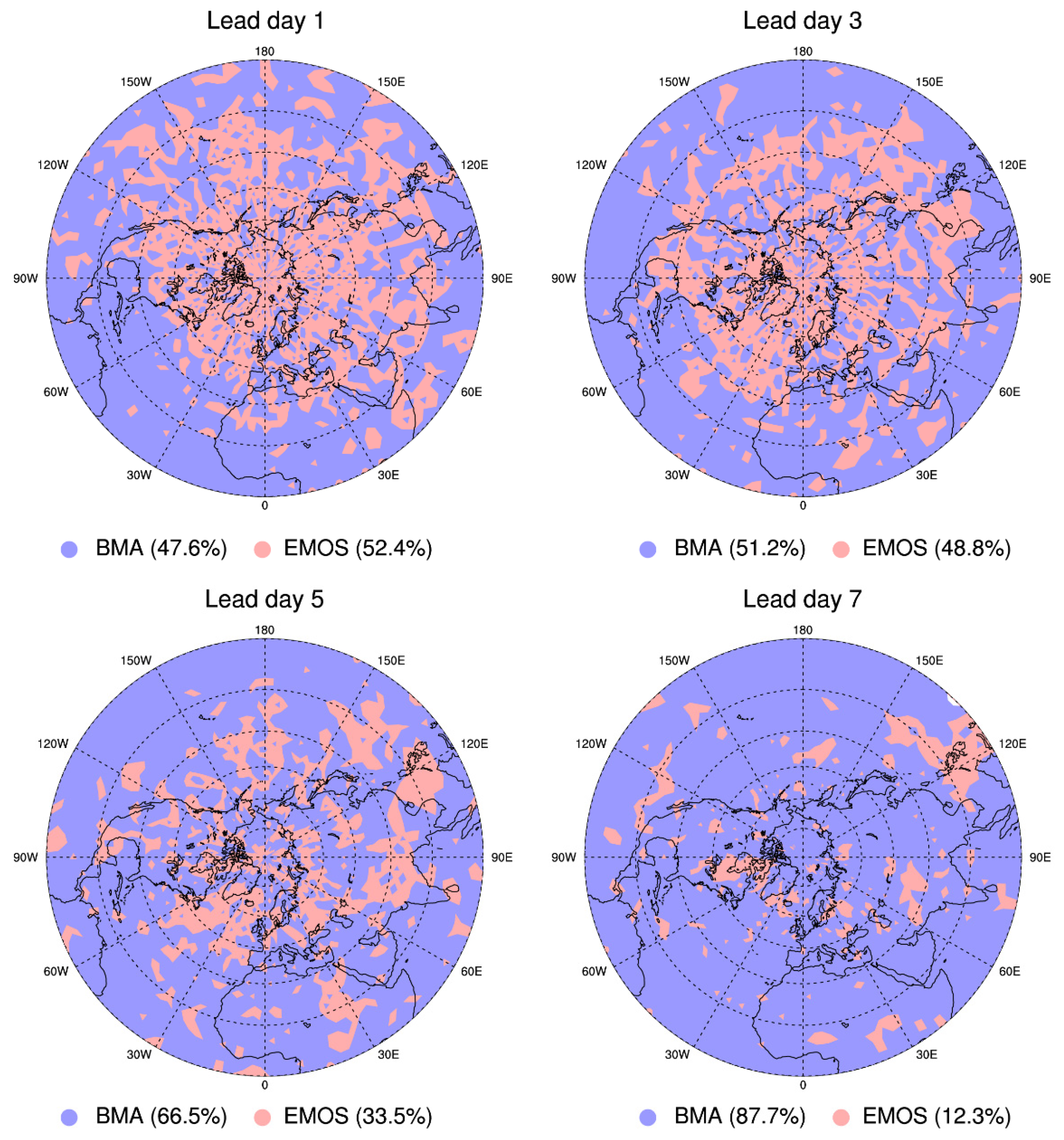
To compare the performance of BMA and EMOS more intuitively, Figure 8 shows the maps of the best-performing method in terms of the BSS over the northern hemisphere with different lead times. The performances of BMA and EMOS were similar for shorter lead times. EMOS had a better prediction skill at mid- and high-latitudes, whereas BMA had a better prediction skill at low latitudes. BMA provided the best forecasts for most of the grid points, especially for lead times of 5–7 days.

4. Discussion and Conclusions

We applied two state-of-the-art approaches to improve ensemble-based probabilistic forecasts of the 500 hPa geopotential height over the northern hemisphere. BMA and EMOS prediction models were established based on the TIGGE multi-model ensembles with lead times of 1–7 days. The results obtained from these two statistical post-processing methods were then compared in terms of the deterministic and probabilistic forecasts and compared with the raw ensembles of the ECMWF, NCEP, and UKMO EPSs using the TIGGE datasets.

A sliding temporal window of 45 days before the forecast period was shown to be optimum training period for all lead times in the BMA prediction model. The EMOS prediction model also used the previous 45 days as the training sample for a fair comparison of its performance with that of the BMA prediction model.

From the perspective of deterministic forecasts, the predictions of the 500 hPa geopotential height distribution from BMA and EMOS were much closer to the observations than the deterministic forecasts of the raw EPSs. In the two selected extreme events, BMA and EMOS predicted the WPSH well, with a strong intensity and large area even for a lead time of 7 days. The potential of the BMA and EMOS methods to improve deterministic forecasts shows that it may be possible to apply these two methods to extended-range weather forecasts with lead times of 10–30 days. The pre-rainy season in South China, the meiyu and the rainy season in North China are usually accompanied by northward movement of the WPSH. These regional rainy seasons determine the distribution and evolution of droughts and floods during the flood season in mid- to eastern China. If the circulation at 500 hPa could be predicted correctly, then timing of these three regional rainy seasons could also be predicted better.

The BMA and EMOS methods also provide a better calibrated and sharper PDF than the raw ensembles. The raw ensembles were under-dispersed, whereas the PIT histograms of the BMA and EMOS methods were comparatively uniform. The overall performance of the ECMWF EPS was the best among the three EPSs and had the smallest RMSE and CRPS. For a specific probabilistic forecast event, in which the 500 hPa geopotential height forecast value at each grid point was higher than its climatological value, the BMA and EMOS predictions were both more skillful than the raw ensembles and the climatological forecast in terms of the BS and BSS verification.

In general, the BMA and EMOS methods were similar for lead times of 1–4 days, whereas the performance of EMOS was poorer at longer lead times. This was probably due to the length of the training period. For a fair comparison, the lengths of the training period for the BMA and EMOS prediction models were both set to 45 days for all lead times. However, a 45-day training period may be not suitable for the EMOS method at longer lead times. EMOS is designed based on the model output statistics method and regression techniques. Estimation of the EMOS parameters is strongly dependent on the choice of the training period and the stability of the forecast error of each contributing EPS. Krishnamurti et al. [68] reported that a stable forecast error is a necessary condition for linear regression. Therefore, the optimum length of the training period for EMOS needs to be investigated further.

The use of BMA and EMOS as statistical post-processing methods based on ensemble forecasts therefore improves the quality of 500 hPa geopotential height forecasts. We used the ECMWF, NCEP, and UKMO EPSs, which have relatively high prediction skills. We tried to increase the number of EPSs contributing to the BMA and EMOS prediction models—for example, the China Meteorological Administration EPS—but the results were less good and the poor performance of the China Meteorological Administration EPS made a negative contribution. We therefore suggest that the EPSs used by the BMA and EMOS prediction models should be selected for further study.

References

- Abbe, C. The physical basis of long-range weather forecasts. Mon. Weather Rev. 1901, 29, 551–561. [Google Scholar] [CrossRef]
- Bjerknes, V. Das Problem der Wettervorhersage betrachtet vom Standpunkt der Mechanik und Physik. Meteorol. Z. 1904, 21, 1–7. [Google Scholar]
- Lorenz, E.N. Deterministic nonperiodic flow. J. Atmos. Sci. 1963, 20, 130–141. [Google Scholar] [CrossRef] [Green Version]
- Lorenz, E.N. Atmospheric predictability as revealed by naturally occurring analogues. J. Atmos. Sci. 1969, 26, 636–646. [Google Scholar] [CrossRef] [Green Version]
- Thompson, P.D. Uncertainty of initial state as a factor in the predictability of large scale atmospheric flow patterns. Tellus 1957, 9, 275–295. [Google Scholar] [CrossRef]
- Smagorinsky, J. Problems and promises of deterministic extended range forecasting. Bull. Am. Meteorol. Soc. 1969, 50, 286–312. [Google Scholar] [CrossRef]
- Hallenbeck, C. Forecasting Precipitation in Percentages of Probability. Mon. Weather Rev. 1920, 48, 645–647. [Google Scholar] [CrossRef]
- Krzysztofowicz, R. The case for probabilistic forecasting in hydrology. J. Hydrol. 2001, 249, 2–9. [Google Scholar] [CrossRef]
- McGovern, A.; Elmore, K.; Gagne, D.J.; Haupt, S.E.; Karstens, C.D.; Lagerquist, R.; Smith, T.; Williams, J.K. Using artificial intelligence to improve real-time decision-making for high-impact weather. Bull. Am. Meteorol. Soc. 2017, 98, 2073–2090. [Google Scholar] [CrossRef]
- Worsnop, R.P.; Scheuerer, M.; Hamill, T.M. Extended-Range Probabilistic Fire-Weather Forecasting Based on Ensemble Model Output Statistics and Ensemble Copula Coupling. Mon. Weather Rev. 2020, 148, 499–521. [Google Scholar] [CrossRef]
- Räisänen, J.; Ruokolainen, L. Probabilistic forecasts of near-term climate change based on a resampling ensemble technique. Tellus 2006, 58A, 461–472. [Google Scholar] [CrossRef] [Green Version]
- Majumdar, S.J.; Torn, R.D. Probabilistic verification of global and mesoscale ensemble forecasts of tropical cyclogenesis. Weather Forecast. 2014, 29, 1181–1198. [Google Scholar] [CrossRef]
- Scheuerer, M.; Gregory, S.; Hamill, T.M.; Shafer, P.E. Probabilistic precipitation-type forecasting based on GEFS ensemble forecasts of vertical temperature profiles. Mon. Weather Rev. 2017, 145, 1401–1412. [Google Scholar] [CrossRef]
- Evans, C.; Van Dyke, D.F.; Lericos, T. How Do Forecasters Utilize Output from a Convection-Permitting Ensemble Forecast System? Case Study of a High-Impact Precipitation Event. Weather Forecast. 2014, 29, 466–486. [Google Scholar] [CrossRef]
- Loeser, C.F.; Herrera, M.A.; Szunyogh, I. An Assessment of the Performance of the Operational Global Ensemble Forecast Systems in Predicting the Forecast Uncertainty. Weather Forecast. 2017, 32, 149–164. [Google Scholar] [CrossRef]
- Schwartz, C.S.; Romine, G.S.; Smith, K.R.; Weisman, M.L. Characterizing and optimizing precipitation forecasts from a convection-permitting ensemble initialized by a mesoscale ensemble Kalman filter. Weather Forecast. 2014, 29, 1295–1318. [Google Scholar] [CrossRef] [Green Version]
- Weyn, J.A.; Durran, D.R. Ensemble Spread Grows More Rapidly in Higher-Resolution Simulations of Deep Convection. J. Atmos. Sci. 2018, 75, 3331–3345. [Google Scholar] [CrossRef]
- Gneiting, T.; Raftery, A.E. Weather forecasting with ensemble methods. Science 2005, 310, 248–249. [Google Scholar] [CrossRef] [Green Version]
- Yussouf, N.; Stensrud, D.J. Prediction of near-surface variables at independent locations from a bias-corrected ensemble forecasting system. Mon. Weather Rev. 2006, 134, 3415–3424. [Google Scholar] [CrossRef]
- Chen, C.H.; Li, C.Y.; Tan, Y.K.; Wang, T. Research of the multi-model super-ensemble prediction based on crossvalidation. J. Meteor. Res. 2010, 68, 464–476. [Google Scholar]
- Hagedorn, R.; Buizza, R.; Hamill, T.M.; Leutbecher, M.; Palmer, T.N. Comparing TIGGE multipmodel forecasts with reforecast-calibrated ECMWF ensemble forecasts. Q. J. R. Meteorol. Soc. 2012, 138, 1814–1827. [Google Scholar] [CrossRef]
- Roulin, E.; Vannitsem, S. Postprocessing of ensemble precipitation predictions with extended logistic regression based on hindcasts. Mon. Weather Rev. 2012, 140, 874–888. [Google Scholar] [CrossRef]
- Zhi, X.F.; Ji, X.D.; Zhang, J.; Zhang, L.; Bai, Y.Q.; Lin, C.Z. Multi-model ensemble forecasts of surface air temperature and precipitation using TIGEE datasets (in Chinese). Trans. Atmos. Sci. 2013, 36, 257–266. [Google Scholar]
- Zhi, X.F.; Qi, H.X.; Bai, Y.Q.; Lin, C.Z. A comparison of three kinds of multi-model ensemble forecast techniques based on the TIGGE data. J. Meteor. Res. 2012, 26, 41–51. [Google Scholar]
- Hamill, T.M.; Scheuerer, M.; Bates, G.T. Analog probabilistic precipitation forecasts using GEFS reforecasts and climatology calibrated precipitation analyses. Mon. Weather Rev. 2015, 143, 3300–3309. [Google Scholar] [CrossRef] [Green Version]
- Zhang, L.; Zhi, X.F. Multi-model consensus forecasting of low temperature and icy weather over central and southern China in early 2008. J. Trop. Meteor. 2015, 21, 67–75. [Google Scholar]
- Slater, L.J.; Villarini, G.; Bradley, A.A. Weighting of NMME temperature and precipitation forecasts across Europe. J. Hydrol. 2017, 552, 646–659. [Google Scholar] [CrossRef] [Green Version]
- Gneiting, T.; Raftery, A.E.; Westveld III, A.H.; Goldman, T. Calibrated probabilistic forecasting using ensemble model output statistics and minimum CRPS estimation. Mon. Weather Rev. 2005, 133, 1098–1118. [Google Scholar] [CrossRef]
- Scheuerer, M. Probabilistic quantitative precipitation forecasting using ensemble model output statistics. Q. J. R. Meteorol. Soc. 2014, 140, 1086–1096. [Google Scholar] [CrossRef] [Green Version]
- Scheuerer, M.; Hamill, T.M. Statistical postprocessing of ensemble precipitation forecasts by fitting censored, shifted gamma distributions. Mon. Weather Rev. 2015, 143, 4578–4596. [Google Scholar] [CrossRef]
- Raftery, A.E.; Gneiting, T.; Balabdaoui, F.; Polakowski, M. Using Bayesian model averaging to calibrate forecast ensembles. Mon. Weather Rev. 2005, 133, 1155–1174. [Google Scholar] [CrossRef] [Green Version]
- Sloughter, J.M.; Raftery, A.E.; Gneiting, T.; Fraley, C. Probabilistic quantitative precipitation forecasting using Bayesian model averaging. Mon. Weather Rev. 2007, 135, 3209–3220. [Google Scholar] [CrossRef]
- Sloughter, J.M.; Gneiting, T.; Raftery, A.E. Probabilistic wind speed forecasting using ensembles and Bayesian model averaging. J. Am. Stat. Assoc. 2010, 105, 25–35. [Google Scholar] [CrossRef] [Green Version]
- Duan, Q.; Ajami, N.K.; Gao, X.; Sorooshian, S. Multi-model ensemble hydrologic prediction using Bayesian model averaging. Adv. Water Resour. 2007, 30, 1371–1386. [Google Scholar] [CrossRef] [Green Version]
- Wilson, L.J.; Beauregard, S.; Raftery, A.E.; Verret, R. Calibrated surface temperature forecasts from the Canadian ensemble prediction system using Bayesian model averaging. Mon. Weather Rev. 2007, 135, 1364–1385. [Google Scholar] [CrossRef] [Green Version]
- Zhang, X.; Srinivasan, R.; Bosch, D. Calibration and uncertainty analysis of the SWAT model using Genetic Algorithms and Bayesian Model Averaging. J. Hydrol. 2009, 374, 307–317. [Google Scholar] [CrossRef]
- Fraley, C.; Raftery, A.E.; Gneiting, T. Calibrating multimodel forecast ensembles with exchangeable and missing members using Bayesian model averaging. Mon. Weather Rev. 2010, 138, 190–202. [Google Scholar] [CrossRef] [Green Version]
- Thorarinsdottir, T.L.; Gneiting, T. Probabilistic forecasts of wind speed: Ensemble model output statistics by using heteroscedastic censored regression. J. R. Stat. Soc. Ser. A Stat. Soc. 2010, 173, 371–388. [Google Scholar] [CrossRef]
- Schuhen, N.; Thorarinsdottir, T.L.; Gneiting, T. Ensemble model output statistics for wind vectors. Mon. Weather Rev. 2012, 140, 3204–3219. [Google Scholar] [CrossRef] [Green Version]
- Hemri, S.; Scheuerer, M.; Pappenberger, F.; Bogner, K.; Haiden, T. Trends in the predictive performance of raw ensemble weather forecasts. Geophys. Res. Lett. 2014, 41, 9197–9205. [Google Scholar] [CrossRef]
- Liu, J.G.; Xie, Z.H. BMA probabilistic quantitative precipitation forecasting over the Huaihe basin using TIGGE multimodel ensemble forecasts. Mon. Weather Rev. 2014, 142, 1542–1555. [Google Scholar] [CrossRef] [Green Version]
- Scheuerer, M.; König, G. Gridded, locally calibrated, probabilistic temperature forecasts based on ensemble model output statistics. Q. J. R. Meteorol. Soc. 2014, 140, 2582–2590. [Google Scholar] [CrossRef]
- Junk, C.; Delle Monache, L.; Alessandrini, S. Analog-based ensemble model output statistics. Mon. Weather Rev. 2015, 143, 2909–2917. [Google Scholar] [CrossRef]
- Baran, S.; Nemoda, D. Censored and shifted gamma distribution based EMOS model for probabilistic quantitative precipitation forecasting. Environmetrics 2016, 27, 280–292. [Google Scholar] [CrossRef] [Green Version]
- Taillardat, M.; Mestre, O.; Zamo, M.; Naveau, P. Calibrated ensemble forecasts using quantile regression forests and ensemble model output statistics. Mon. Weather Rev. 2016, 144, 2375–2393. [Google Scholar] [CrossRef]
- Vogel, P.; Knippertz, P.; Fink, A.H.; Schlueter, A.; Gneiting, T. Skill of global raw and postprocessed ensemble predictions of rainfall over northern tropical Africa. Weather Forecast. 2018, 33, 369–388. [Google Scholar] [CrossRef]
- Ji, L.Y.; Zhi, X.F.; Zhu, S.P.; Fraedrich, K. Probabilistic precipitation forecasting over East Asia using Bayesian model averaging. Weather Forecast. 2019, 34, 377–392. [Google Scholar] [CrossRef]
- Kidson, J.W. Indices of the Southern Hemisphere zonal wind. J. Clim. 1988, 1, 183–194. [Google Scholar] [CrossRef] [Green Version]
- Kożuchowski, K.; Wibig, J.; Maheras, P. Connections between air temperature and precipitation and the geopotential height of the 500 hPa level in a meridional cross-section in Europe. Int. J. Climatol. 1992, 12, 343–352. [Google Scholar] [CrossRef]
- Simmonds, I. Modes of atmospheric variability over the Southern Ocean. J. Geophys. Res. 2003, 108, 8078. [Google Scholar] [CrossRef]
- Zheng, X.; Frederiksen, C.S. Statistical prediction of seasonal mean Southern Hemisphere 500-hPa geopotential heights. J. Clim. 2007, 20, 2791–2809. [Google Scholar] [CrossRef]
- Sun, C.; Li, J. Space–time spectral analysis of the Southern Hemisphere daily 500-hPa geopotential height. Mon. Weather Rev. 2012, 140, 3844–3856. [Google Scholar] [CrossRef] [Green Version]
- Qiao, S.; Zou, M.; Cheung, H.N.; Zhou, W.; Li, Q.; Feng, G.; Dong, W. Predictability of the wintertime 500 hPa geopotential height over Ural-Siberia in the NCEP climate forecast system. Clim. Dyn. 2020, 54, 1591–1606. [Google Scholar] [CrossRef]
- Fisher, R.A. On the mathematical foundations of theoretical statistics. Philos. Trans. R. Soc. Lond. 1992, 222A, 309–368. [Google Scholar]
- Zhi, X.F.; Lin, C.Z.; Bai, Y.Q.; Qi, H.X. Superensemble forecasts of the surface temperature in Northern Hemisphere middle latitudes (in Chinese). Sci. Meteorol. Sin. 2009, 29, 569–574. [Google Scholar]
- Brier, G.W. Verification of forecasts expressed in terms of probability. Mon. Weather Rev. 1950, 78, 1–3. [Google Scholar] [CrossRef]
- Sanders, F. On subjective probability forecasting. J. Appl. Meteor. 1963, 2, 191–201. [Google Scholar] [CrossRef] [Green Version]
- Hamill, T.M.; Juras, J. Measuring forecast skill: Is it real skill or is it the varying climatology? Q. J. R. Meteorol. Soc. 2006, 132, 2905–2923. [Google Scholar] [CrossRef] [Green Version]
- Hu, Y.M.; Zhai, P.M.; Luo, X.L.; Lv, J.M.; Qin, Z.N.; Hao, Q.C. Large scale circulation and low frequency signal characteristic for the persistent extreme precipitation in the first rainy season over South China in 2013. Acta Meteorol. Sin. 2014, 72, 465–477. (In Chinese) [Google Scholar]
- Wu, H.; Zhai, P.M.; Chen, Y. A comprehensive classification of anomalous circulation patterns responsible for persistent precipitation extremes in South China. J. Meteor. Res. 2016, 30, 483–495. [Google Scholar] [CrossRef]
- Sun, Y.; Zhang, X.; Zwiers, F.W.; Song, L.; Wan, H.; Hu, T.; Yin, H.; Ren, G. Rapid increase in the risk of extreme summer heat in Eastern China. Nat. Clim. Chang. 2014, 4, 1082–1085. [Google Scholar] [CrossRef]
- Wang, W.; Zhou, W.; Li, X.; Wang, X.; Wang, D. Synoptic-scale characteristics and atmospheric controls of summer heat waves in China. Clim. Dyn. 2016, 46, 2923–2941. [Google Scholar] [CrossRef]
- Gneiting, T.; Balabdaoui, F.; Raftery, A.E. Probabilistic forecasts, calibration and sharpness. J. R. Stat. Soc. Ser. B 2007, 69, 243–268. [Google Scholar] [CrossRef] [Green Version]
- Talagrand, O.; Vautard, R.; Strauss, B. Evaluation of Probabilistic Prediction Systems; European Centre for Medium-Range Weather Forecasts: Reading, UK, 1997; pp. 1–25. [Google Scholar]
- Hamill, T.M. Interpretation of Rank Histograms for Verifying Ensemble Forecasts. Mon. Weather Rev. 2001, 129, 550–560. [Google Scholar] [CrossRef]
- Hamill, T.M.; Hagedorn, R.; Whitaker, J.S. Probabilistic forecast calibration using ECMWF and GFS ensemble reforecasts. Part II: Precipitation. Mon. Weather Rev. 2008, 136, 2620–2632. [Google Scholar] [CrossRef] [Green Version]
- Wilks, D.S. The calibration simplex: A generalization of the reliability diagram for three-category probability forecasts. Weather Forecast. 2013, 28, 1210–1218. [Google Scholar] [CrossRef]
- Krishnamurti, T.N.; Kishtawal, C.M.; Zhang, Z.; LaRow, T.; Bachiochi, D.; Williford, E.; Gadgil, S.; Surendran, S. Multimodel ensemble forecasts for weather and seasonal climate. J. Clim. 2000, 13, 4196–4216. [Google Scholar] [CrossRef]
Figure 1.
Mean 500 hPa geopotential height distribution from 23 April to 30 May 2013 for (a) the observations, the difference between the observations and the ensemble mean of the (b) European Centre for Medium-Range Weather Forecasts (ECMWF), (c) National Centers for Environmental Prediction (NCEP), and (d) UK Met Office (UKMO) ensemble prediction systems (EPSs) with a lead time of 7 days and the difference between the observations and the deterministic forecast of the (e) Bayesian model averaging (BMA) and (f) ensemble model output statistics (EMOS) with a lead time of 7 days. The root mean square error and anomaly correlation coefficient between the forecasts and the observations are shown in the upper right-hand corner of each part. The purple labels denote the place named Ural Mountains, Lake Baikal, Yellow, and Huaihe river basins (YH), and Xinjiang regions.
Figure 2.
Mean 500 hPa geopotential height distribution from 1 July to 20 August 2013 for (a) the observations, the difference between the observations and the ensemble mean of the (b) ECMWF, (c) NCEP and (d) UKMO EPSs with a lead time of 7 days and the difference between the observations and the deterministic forecast of the (e) BMA and (f) EMOS with a lead time of 7 days. The root mean square error and anomaly correlation coefficient between the forecasts and the observations are shown in the upper right-hand corner of each part. The purple box denotes the South China region.
Figure 3.
Predictive probability density function (PDF) of the 500 hPa geopotential height for (72.5° N, 42.5° E) on 8 July 2013 obtained from the BMA, EMOS and raw ensemble forecasts with lead times of (a) 1 day and (b) 7 days. The red vertical line represents the verifying observation. The BMA weights of ECMWF, NCEP, and UKMO EPSs with lead time of 1 day (7 days) are 0.3052 (0.4195), 0.32 (0.3431), and 0.3749 (0.2375), respectively.
Figure 4.
Verification rank histograms for the ECMWF EPS forecasts and the PIT histograms for the BMA and EMOS forecast distributions of the 500 hPa geopotential height with different lead times.
Figure 5.
Mean verification for the BMA, EMOS and raw EPS forecasts of the 500 hPa geopotential height with lead times of 1–7 days (units: gpm) for the (a) RMSE and (b) continuous ranked probability score (CRPS).
Figure 6.
(a) Brier score and (b) Brier skill score of probabilistic forecasts of the 500 hPa geopotential height higher than the climatology values by the BMA, EMOS, and raw ensemble forecasts with lead times of 1–7 days.
Figure 7.
Reliability diagram of the binned probabilistic forecast versus the observed relative frequency of the 500 hPa geopotential height higher than its climatology value for consensus voting of the raw ensemble, BMA and EMOS forecasts with a lead time of 1 day. The black diagonal line is the perfect forecast.
Figure 8.
Distribution of the best-performing post-processing methods over the northern hemisphere in terms of the Brier score at different lead times. The percentage of the best-performing post-processing methods is listed under each part.