
A Review of Operational Ensemble Forecasting Efforts in the United States Air Force

Abstract
:1. Introduction
“The chaotic character of the atmosphere, coupled with inevitable inadequacies in observations and computer models, results in forecasts that always contain uncertainties. These uncertainties generally increase with forecast lead time and vary with weather situation and location. Uncertainty is thus a fundamental characteristic of weather...and no forecast is complete without a description of its uncertainty.”
“...some operators may refuse to accept weather forecasts worded in probabilistic terms...Unfortunately, this attitude makes the forecaster—not the operator—the decision-maker.”
2. Development Era (2004–2008)
2.1. Methods
2.2. Results
- −
- Ensemble Transform Kalman Filter methods generally performed better than Perturbed Observations
- −
- All methods of accounting for model uncertainty improved forecast skill at least marginally
- −
- Model physics diversity was critical for increasing/obtaining forecast skill in variables in the planetary boundary layer
- −
- Utilizing Stochastic Backscatter provided for the highest degree of skill in variables aloft
- −
- Diverse physics, parameter perturbations, and backscatter employed together led to the most skillful ensemble
3. CAM Era (2008–2015)
3.1. Methods
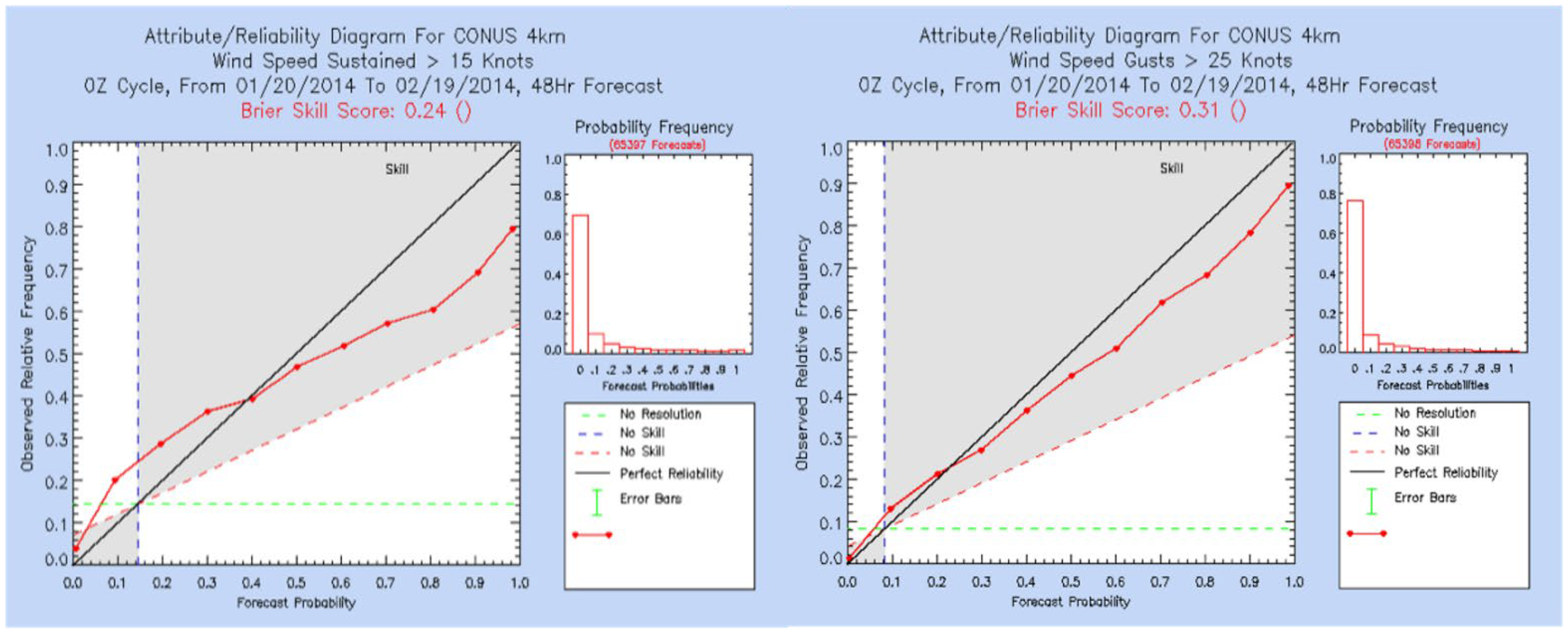
3.2. Results
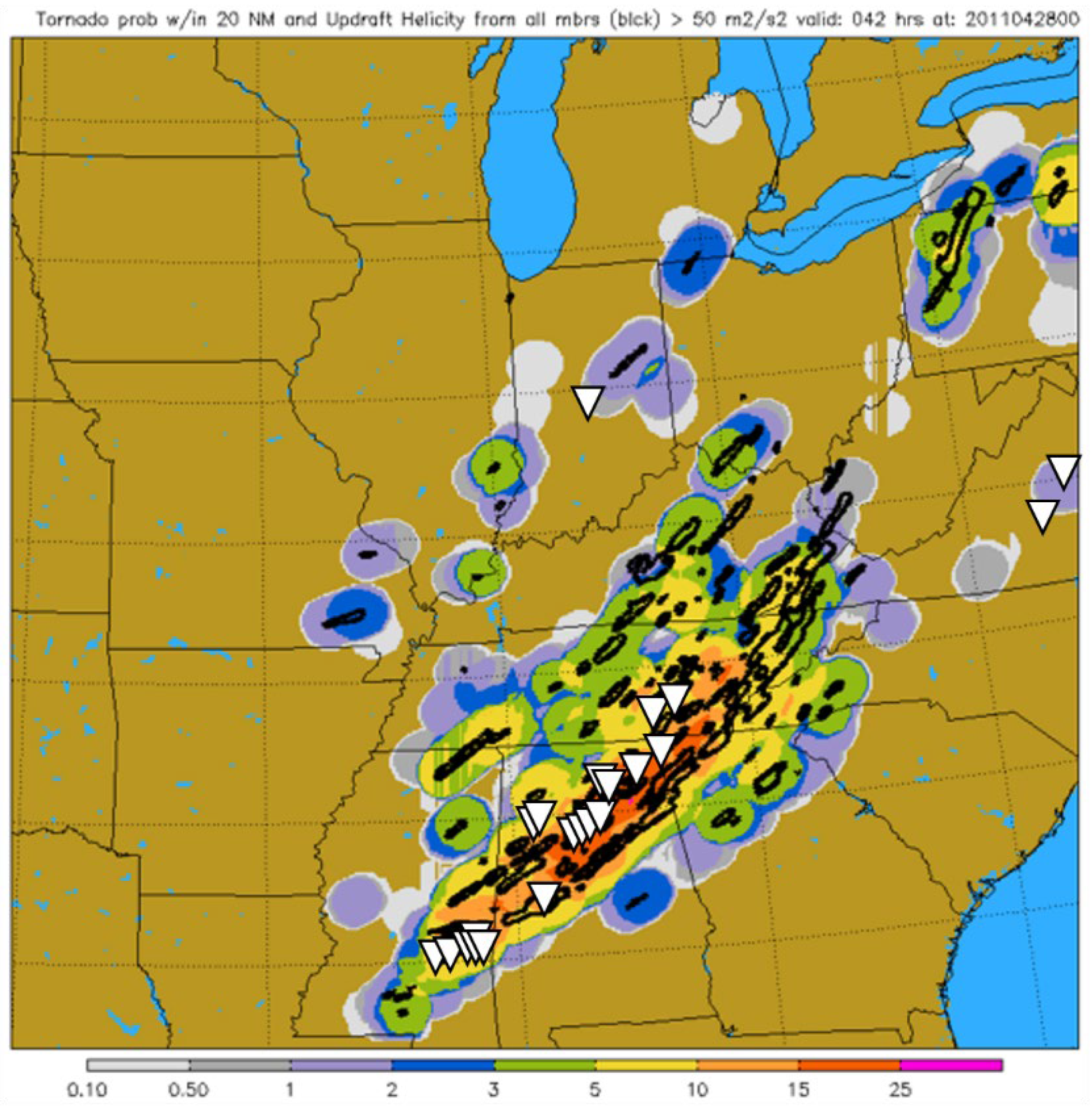
3.2.1. US Tornado Outbreaks—April 2011 and 2012
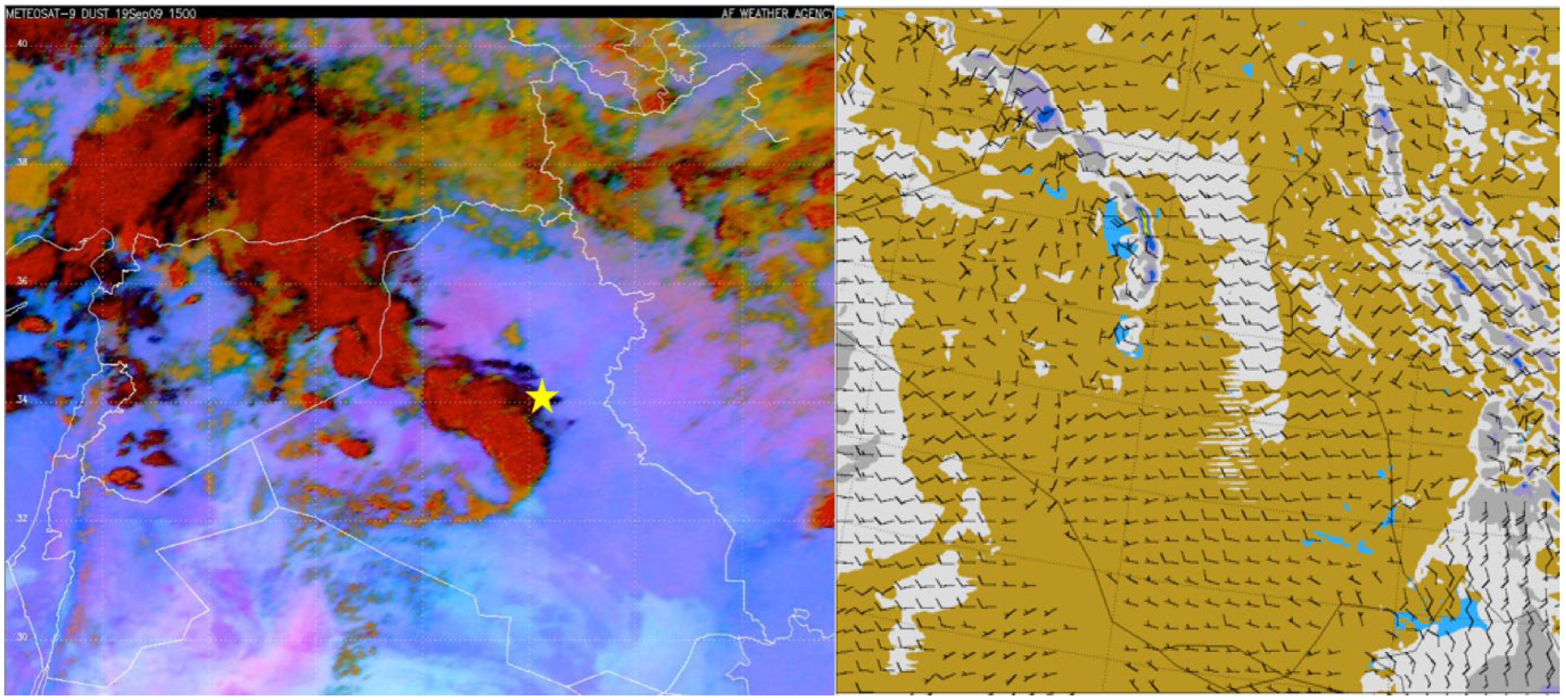
3.2.2. Iraq Convective Dust—19 September 2009
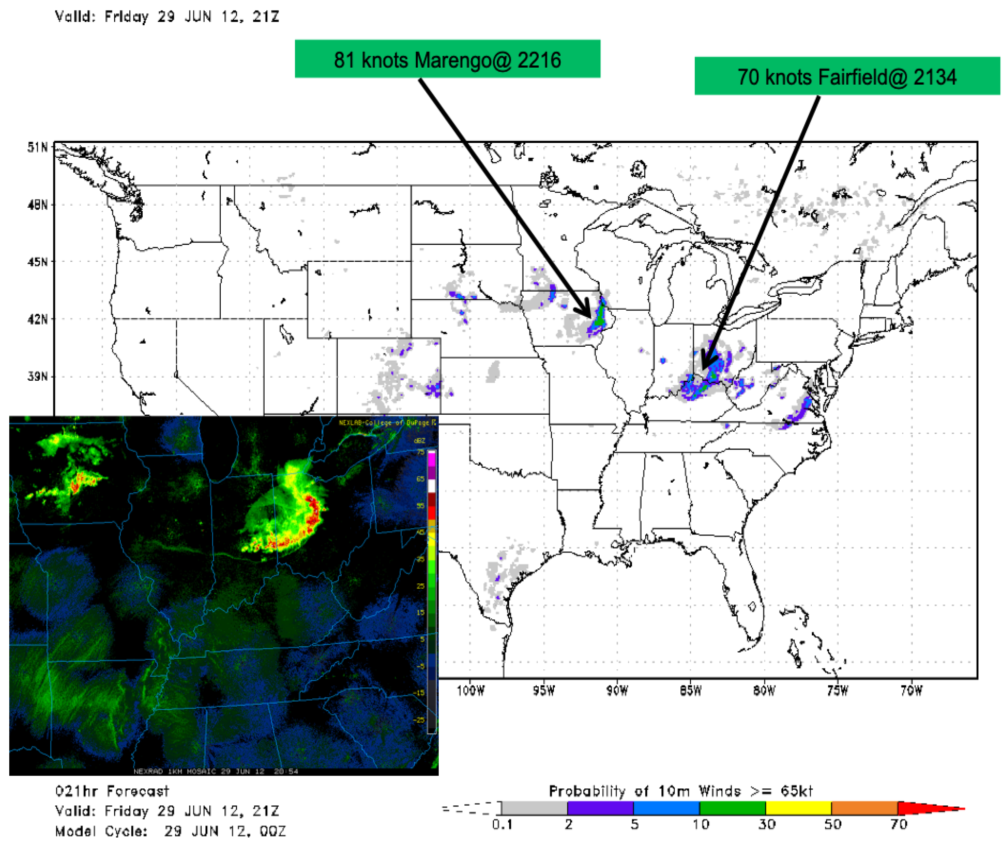
3.2.3. Derecho—29 June 2012
3.2.4. Afghanistan Dust in Variable Terrain
3.2.5. External Studies
3.2.6. Internal Studies
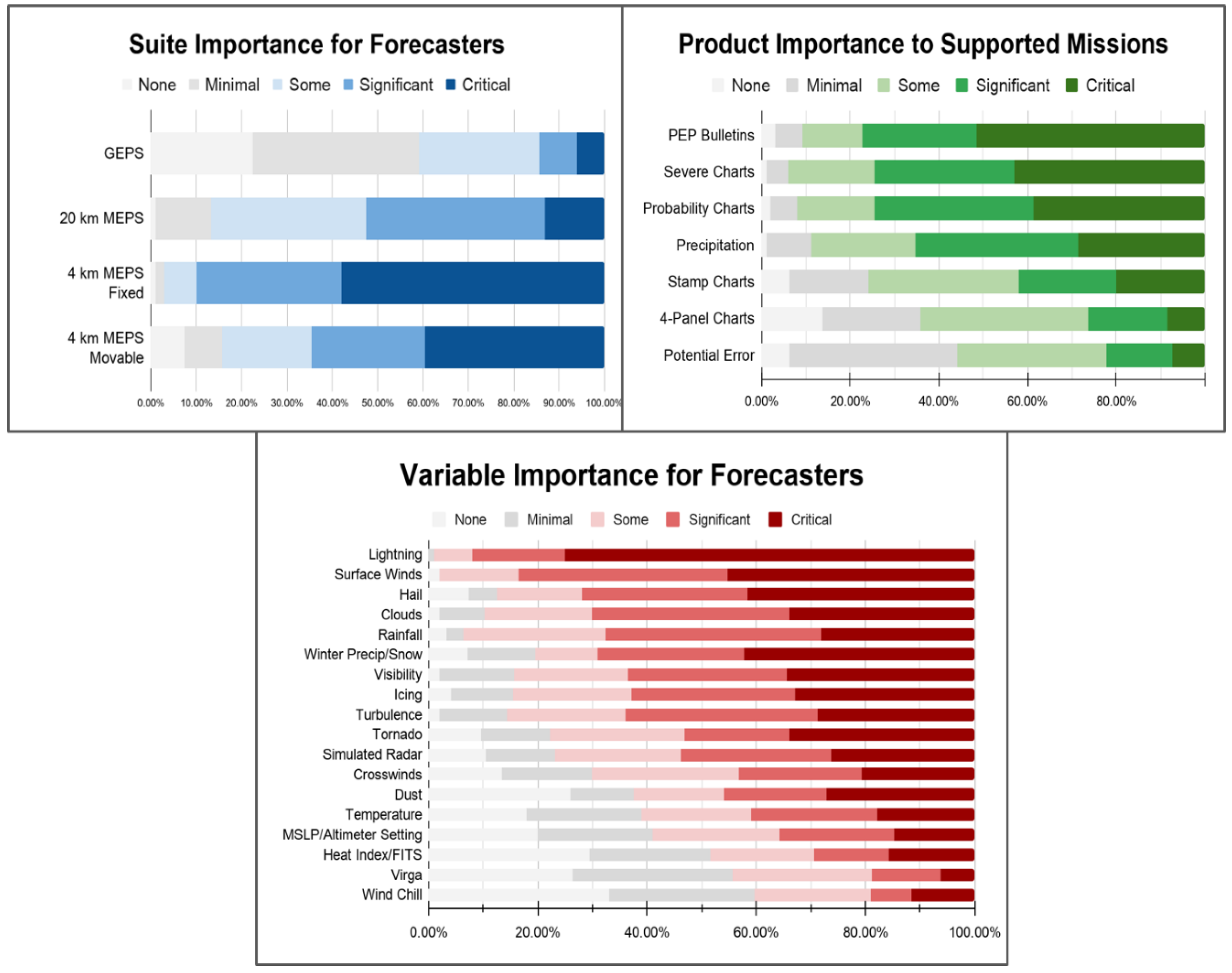
3.2.7. User Feedback
4. Rolling Ensemble (2015–Present)
4.1. Methods
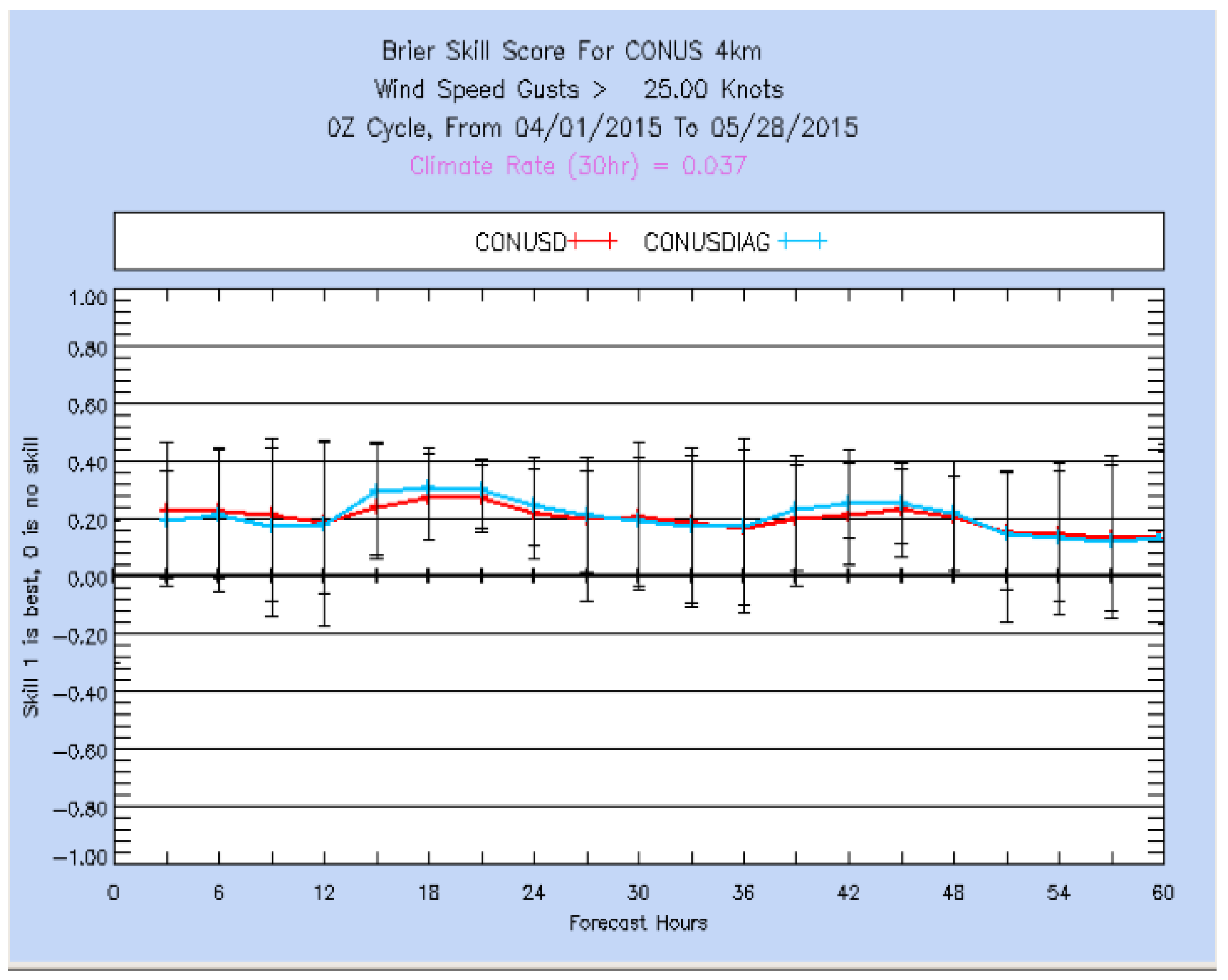
4.2. Results
5. Conclusions
5.1. Ensemble Design
“By studying the same model formulation across a range of timescales and system applications, one can learn about the rate of growth and nature of both model errors and desirable behaviours. Also, by constraining configurations to perform adequately across a wide variety of systems, scientists can be more confident that model developments seen to improve performance metrics in any one system are doing so by modelling a truer representation of the real atmosphere.”
“Even if a given multimodel ensemble is unable to bound truth, if each ensemble member is consistent with its model attractor, the ensemble’s distribution can provide information about the sensitivity of regions of state space to the different models making up the ensemble.”
5.2. Scientific Rigor in an Operational Environment
5.3. Post-Processing
5.4. Future Efforts
Author Contributions
Funding
Institutional Review Board Statement
Informed Consent Statement
Data Availability Statement
Acknowledgments
Conflicts of Interest
References
- Cox, J.D. Storm Watchers: The Turbulent History of Weather Prediction from Franklin’s Kite to El Niño; John Wiley: Hoboken, NJ, USA, 2002. [Google Scholar]
- Benson, J.T. Weather and the Wreckage at Desert-One. Air Space Power J. 2007. Available online: https://www.airuniversity.af.edu/Portals/10/ASPJ/journals/Chronicles/benson.pdf (accessed on 21 February 2007).
- Kamarck, E. The Iranian Hostage Crisis and Its Effect on American Politics. Brookings. 4 November 2019. Available online: https://www.brookings.edu/blog/order-from-chaos/2019/11/04/the-iranian-hostage-crisis-and-its-effect-on-american-politics/ (accessed on 12 March 2021).
- Nobis, T. Conclusions of Weather in Battle History Survey; Internal Document; Air Force Research Laboratory: Rome, NY, USA, 2010. [Google Scholar]
- National Research Council. Completing the Forecast: Characterizing and Communicating Uncertainty for Better Decisions Using Weather and Climate Forecasts; The National Academies Press: Washington, DC, USA, 2006. [Google Scholar] [CrossRef]
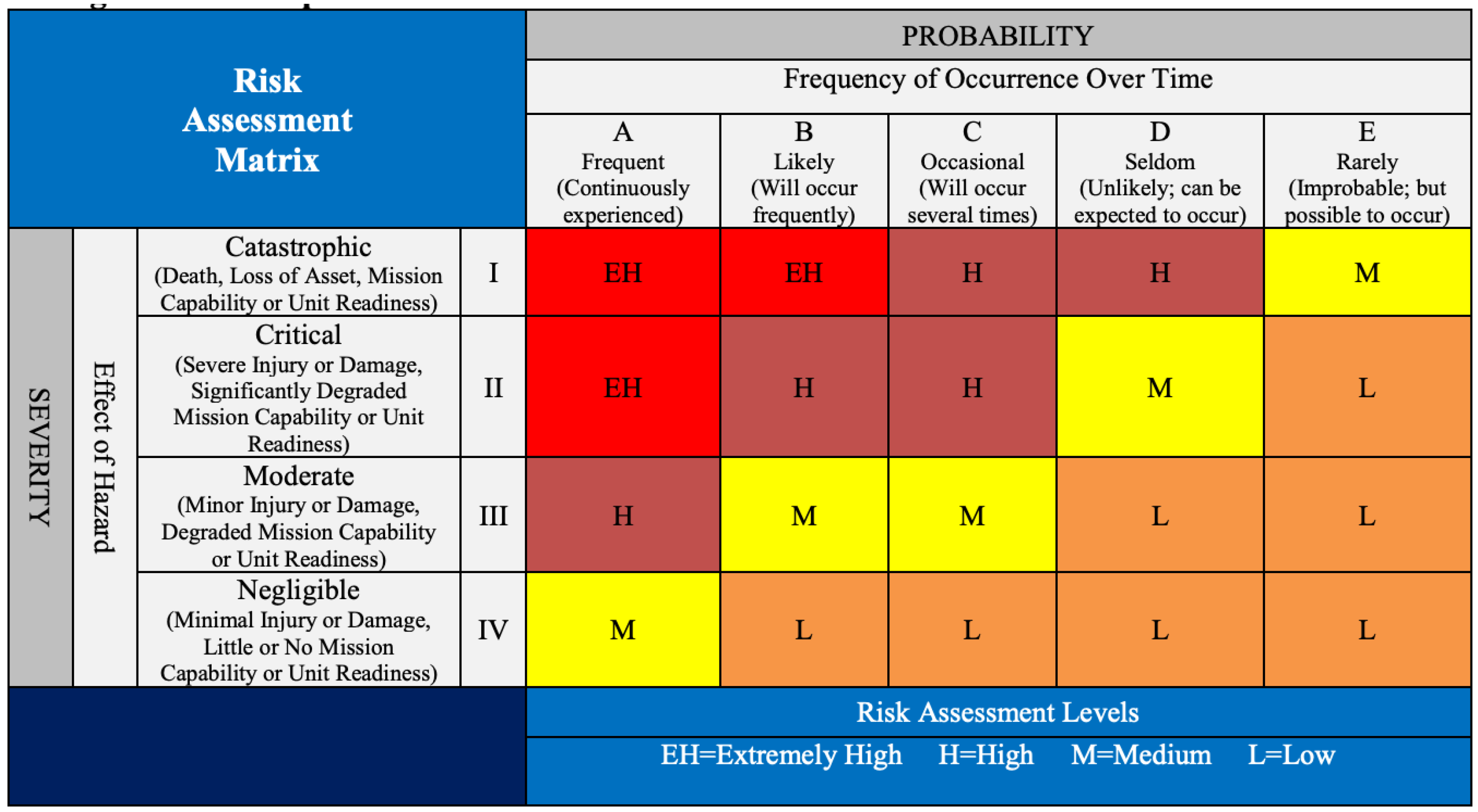
- United States Department of Defense; Department of the Air Force. Air Force Instruction 90-802: Risk Management. Available online: https://static.e-publishing.af.mil/production/1/af_se/publication/afi90-802/afi90-802.pdf (accessed on 1 April 2019).
- United States Department of Defense; Department of the Air Force. Air Force Manual 15-129: Air and Space Weather Operations. Available online: https://static.e-publishing.af.mil/production/1/af_a3/publication/afman15-129/afman15-129.pdf (accessed on 9 July 2020).
- Thompson, J.C. On the Operational Deficiencies in Categorical Weather Forecasts. Bull. Am. Meteorol. Soc. 1952, 33, 223–226. [Google Scholar] [CrossRef]
- Scruggs, F.P. Decision Theory and Weather Forecasts: A Union with Promise. Air University Review. July–August 1967. Available online: https://web.archive.org/web/20170126062712/http://www.airpower.maxwell.af.mil/airchronicles/aureview/1967/jul-aug/scruggs.html (accessed on 22 March 2021).
- Murphy, A.H.; Katz, R.W.; Winkler, R.L.; Hsu, W.-R. Repetitive Decision Making and the Value of Forecasts in the Cost?Loss Ratio Situation: A Dynamic Model. Mon. Weather Rev. 1985, 113, 801–813. [Google Scholar] [CrossRef] [Green Version]
- Pielke, R.A. Who decides? Forecasts and responsibilities in the 1997 Red River flood. Appl. Behav. Sci. Rev. 1999, 7, 83–101. [Google Scholar] [CrossRef]
- Zhu, Y.; Toth, Z.; Wobus, R.; Richardson, D.; Mylne, K. The Economic Value Of Ensemble-Based Weather Forecasts. Bull. Am. Meteorol. Soc. 2002, 83, 73–83. [Google Scholar] [CrossRef]
- Eckel, F.A.; Cunningham, J.G.; Hetke, D.E. Weather and the Calculated Risk: Exploiting Forecast Uncertainty for Operational Risk Management. Air Space Power J. 2008, 22, 71–82. [Google Scholar]
- United States Government Accountability Office. Weapon Systems Annual Assessment: Limited Use of Knowledge-Based Practices Continues to Undercut DOD’s Investments. Available online: https://www.gao.gov/products/gao-19-336sp (accessed on 7 May 2019).
- United States Government Accountability Office. Defense Real Property: DOD Needs to Take Additional Actions to Improve Management of Its Inventory Data. Available online: https://www.gao.gov/products/gao-19-73 (accessed on 13 November 2018).
- Lazo, J.K.; Lawson, M.; Larsen, P.H.; Waldman, D.M. U.S. Economic Sensitivity to Weather Variability. Bull. Am. Meteorol. Soc. 2011, 92, 709–720. [Google Scholar] [CrossRef] [Green Version]
- Shapiro, A. Tyndall Air Force Base Still Faces Challenges In Recovering From Hurricane Michael. NPR Organization. Available online: https://www.npr.org/2019/05/31/728754872/tyndall-air-force-base-still-faces-challenges-in-recovering-from-hurricane-micha (accessed on 12 March 2021).
- Mizokami, K. Hurricane Michael Mangled at Least 17 F-22 Raptors That Failed to Flee Their Base. Popular Mechanics. 15 October 2018. Available online: https://www.popularmechanics.com/military/aviation/a23792532/f-22s-damaged-destroyed-hurricane-michael/ (accessed on 12 March 2021).
- 309th AMARG the First FAA Military Repair Station in AFSC. Standard-Examiner. Available online: https://www.standard.net/hilltop/news/309th-amarg-the-first-faa-military-repair-station-in-afsc/article_8e2bbf9b-de36-5a90-a57b-746c9d076b88.html (accessed on 12 March 2021).
- Liewer, S. Tornado Caused Almost $20 Million in Damage at Offutt Air Force Base. Available online: https://omaha.com/news/military/tornado-caused-almost-20-million-in-damage-at-offutt-air-force-base/article_dc05a175-0658-5595-b585-9f09f878e4b6.html (accessed on 12 March 2021).
- Amadeo, K. Why Military Spending Is More Than You Think It Is. Available online: https://www.thebalance.com/u-s-military-budget-components-challenges-growth-3306320 (accessed on 12 March 2021).
- Kalnay, E. Historical perspective: Earlier ensembles and forecasting forecast skill. Q. J. R. Meteorol. Soc. 2019, 145, 25–34. [Google Scholar] [CrossRef] [Green Version]
- Joslyn, S.L.; Leclerc, J.E. Uncertainty forecasts improve weather-related decisions and attenuate the effects of forecast error. J. Exp. Psychol. Appl. 2012, 18, 126–140. [Google Scholar] [CrossRef] [PubMed]
- Marimo, P.; Kaplan, T.R.; Mylne, K.; Sharpe, M. Communication of Uncertainty in Temperature Forecasts. Weather Forecast 2015, 30, 5–22. [Google Scholar] [CrossRef]
- Hoffman, R.N.; Kalnay, E. Lagged average forecasting, an alternative to Monte Carlo forecasting. Tellus A Dyn. Meteorol. Oceanogr. 1983, 35, 100–118. [Google Scholar] [CrossRef]
- Du, J.; Mullen, S.L.; Sanders, F. Short-Range Ensemble Forecasting of Quantitative Precipitation. Mon. Weather Rev. 1997, 125, 2427–2459. [Google Scholar] [CrossRef]
- Stensrud, D.J.; Brooks, H.E.; Du, J.; Tracton, M.S.; Rogers, E. Using Ensembles for Short-Range Forecasting. Mon. Weather Rev. 1999, 127, 433–446. [Google Scholar] [CrossRef]
- Wandishin, M.S.; Mullen, S.L.; Stensrud, D.J.; Brooks, H.E. Evaluation of a Short-Range Multimodel Ensemble System. Mon. Weather Rev. 2001, 129, 729–747. [Google Scholar] [CrossRef] [Green Version]
- Mylne, K.R.; Evans, R.E.; Clark, R.T. Multi-model multi-analysis ensembles in quasi-operational medium-range forecasting. Q. J. R. Meteorol. Soc. 2002, 128, 361–384. [Google Scholar] [CrossRef]
- Du, J.; McQueen, J.; Geoff DiMego, G.; Black, T.; Juang, H.; Rogers, E.; Ferrier, B.; Zhou, B.; Toth, Z. The NOAA/NWS/NCEP Short Range Ensemble Forecast (SREF) system: Evaluation of an initial condition vs multiple model physics ensemble approach. In Proceedings of the 16th Conference on Numerical Weather Prediction, Seattle, WA, USA, 11–15 January 2004; CD-ROM, 21.3; American Meteor Society: Geneseo, NY, USA.
- Eckel, F.A.; Mass, C.F. Aspects of Effective Mesoscale, Short-Range Ensemble Forecasting. Weather Forecast 2005, 20, 328–350. [Google Scholar] [CrossRef]
- Roebber, P.J.; Schultz, D.M.; Colle, B.A.; Stensrud, D.J. Toward Improved Prediction: High-Resolution and Ensemble Modeling Systems in Operations. Weather Forecast 2004, 19, 936–949. [Google Scholar] [CrossRef]
- Cunningham, J.G. Applying Ensemble Prediction Systems to Department of Defense Operations. Master’s Thesis, Naval Postgraduate School, Monterey, CA, USA, March 2006. Available online: https://apps.dtic.mil/sti/pdfs/ADA445411.pdf (accessed on 22 March 2021).
- Nobis, T.E.; Kuchera, E.L.; Rentschler, S.A.; Rugg, S.A.; Cunningham, J.G.; Synder, C.; Hacker, J.P. Towards the Development of an Operational Mesoscale Ensemble System for the DoD Using the WRF-ARW Model. In Proceedings of the 2008 DoD HPCMP Users Group Conference, Seattle, WA, USA, 14–17 July 2008; pp. 288–292. [Google Scholar]
- Skamarock, W.C.; Skamarock, W.C.; Klemp, J.B.; Dudhia, J.; Gill, D.O.; Barker, D.M.; Wang, W.; Powers, J.G. A description of the Advanced Research WRF Version 2. NCAR Tech. Notes 2005, 88. [Google Scholar] [CrossRef]
- Hodur, R.M. The Naval Research Laboratory’s Coupled Ocean/Atmosphere Mesoscale Prediction System (COAMPS). Mon. Weather Rev. 1997, 125, 1414–1430. [Google Scholar] [CrossRef]
- Wei, M.; Toth, Z.; Wobus, R.; Zhu, Y. Initial perturbations based on the ensemble transform (ET) technique in the NCEP global operational forecast system. Tellus A Dyn. Meteorol. Oceanogr. 2008, 60, 62–79. [Google Scholar] [CrossRef] [Green Version]
- Hacker, J.P.; Ha, S.-Y.; Snyder, C.; Berner, J.; Eckel, F.A.; Kuchera, E.; Pocernich, M.; Rugg, S.; Schramm, J.; Wang, X. The U.S. Air ForceWeather Agency’s mesoscale ensemble: Scientific description and performance results. Tellus A Dyn. Meteorol. Oceanogr. 2011, 63, 625–641. [Google Scholar] [CrossRef] [Green Version]
- Kuchera, E.L.; Nobis, I.; Rugg, S.; Rentschler, S.; Cunningham, J.; Hughesand, H.; Sittel, M. AFWA’s Joint Ensemble System Experiment (JEFS) Experiment. In Proceedings of the 19th Conference on Numerical Weather Prediction, Omaha, NE, USA, 1–9 June 2009; Available online: https://ams.confex.com/ams/pdfpapers/152656.pdf (accessed on 22 March 2021).
- Peng, M.S.; Ridout, J.A.; Hogan, T.F. Recent Modifications of the Emanuel Convective Scheme in the Navy Operational Global Atmospheric Prediction System. Mon. Weather Rev. 2004, 132, 1254–1268. [Google Scholar] [CrossRef]
- Côté, J.; Gravel, S.; Méthot, A.; Patoine, A.; Roch, M.; Staniforth, A. The Operational CMC–MRB Global Environmental Multiscale (GEM) Model. Part I: Design Considerations and Formulation. Mon. Weather Rev. 1998, 126, 1373–1395. [Google Scholar] [CrossRef]
- McCormick, J.R. Near Surface Forecast Challenges at the Air Force Weather Agency. In Proceedings of the 15th Conference on Aviation, Range, and Aerospace Meteorology, Los Angeles, CA, USA, 1 August 2011; Available online: https://ams.confex.com/ams/14Meso15ARAM/webprogram/Manuscript/Paper190769/McCormickPreprint.pdf (accessed on 22 March 2021).
- Hsu, W.-R.; Murphy, A.H. The attributes diagram A geometrical framework for assessing the quality of probability forecasts. Int. J. Forecast 1986, 2, 285–293. [Google Scholar] [CrossRef]
- Wilks, D.S. Statistical Methods in the Atmospheric Sciences, 2nd ed.; Academic Press: Cambridge, MA, USA, 2006. [Google Scholar]
- Arribas, A.; Robertson, K.B.; Mylne, K.R. Test of a Poor Man’s Ensemble Prediction System for Short-Range Probability Forecasting. Mon. Weather Rev. 2005, 133, 1825–1839. [Google Scholar] [CrossRef]
- Palmer, T.N.; Tibaldi, S. On the Prediction of Forecast Skill. Mon. Weather Rev. 1988, 116, 2453–2480. [Google Scholar] [CrossRef] [Green Version]
- Laloux, F. Reinventing Organizations: A Guide to Creating Organizations Inspired by the Next Stage of Human Consciousness; Nelson Parker: Millis, MA, USA, 2014. [Google Scholar]
- Evans, C.; Van Dyke, D.F.; Lericos, T. How Do Forecasters Utilize Output from a Convection-Permitting Ensemble Forecast System? Case Study of a High-Impact Precipitation Event. Weather Forecast 2014, 29, 466–486. [Google Scholar] [CrossRef]
- Brown, A.; Milton, S.; Cullen, M.; Golding, B.; Mitchell, J.F.B.; Shelly, A. Unified Modeling and Prediction of Weather and Climate: A 25-Year Journey. Bull. Am. Meteorol. Soc. 2012, 93, 1865–1877. [Google Scholar] [CrossRef]
- Deutscher Wetterdienst. Ensemble Prediction. Available online: https://www.dwd.de/EN/research/weatherforecasting/num_modelling/04_ensemble_methods/ensemble_prediction/ensemble_prediction_en.html;jsessionid=0E5AD903B9A7A241626C1D35E020FAC9.live31083?nn=484822#COSMO-D2-EPS (accessed on 12 March 2021).
- Rentschler, S.A. Air Force Weather Ensembles. In Proceedings of the 5th NCEP Ensemble Workshop, College Park, MD, USA, 10 May 2011. [Google Scholar]
- Kuchera, E.L. Air Force Weather Ensembles. In Proceedings of the 15th WRF Users Workshop, Boulder, CO, USA, 23–27 June 2014; Available online: https://www2.mmm.ucar.edu/wrf/users/workshops/WS2014/ppts/2.3.pdf (accessed on 22 March 2021).
- Ebert, E.E. Ability of a Poor Man’s Ensemble to Predict the Probability and Distribution of Precipitation. Mon. Weather Rev. 2001, 129, 2461–2480. [Google Scholar] [CrossRef]
- Kain, J.S.; Weiss, S.J.; Bright, D.R.; Baldwin, M.E.; Levit, J.J.; Carbin, G.W.; Schwartz, C.S.; Weisman, M.L.; Droegemeier, K.K.; Weber, D.B.; et al. Some Practical Considerations Regarding Horizontal Resolution in the First Generation of Operational Convection-Allowing NWP. Weather Forecast 2008, 23, 931–952. [Google Scholar] [CrossRef]
- Clark, A.J.; Gallus, W.A.; Xue, M.; Kong, F. A Comparison of Precipitation Forecast Skill between Small Convection-Allowing and Large Convection-Parameterizing Ensembles. Weather Forecast 2009, 24, 1121–1140. [Google Scholar] [CrossRef] [Green Version]
- Schwartz, C.S.; Kain, J.S.; Weiss, S.J.; Xue, M.; Bright, D.R.; Kong, F.; Thomas, K.W.; Levit, J.J.; Coniglio, M.C. Next-Day Convection-Allowing WRF Model Guidance: A Second Look at 2-km versus 4-km Grid Spacing. Mon. Weather Rev. 2009, 137, 3351–3372. [Google Scholar] [CrossRef]
- Clark, A.J.; Gallus, W.A.; Xue, M.; Kong, F. Convection-Allowing and Convection-Parameterizing Ensemble Forecasts of a Mesoscale Convective Vortex and Associated Severe Weather Environment. Weather Forecast 2010, 25, 1052–1081. [Google Scholar] [CrossRef]
- Kain, J.S.; Dembek, S.R.; Weiss, S.J.; Case, J.L.; Levit, J.J.; Sobash, R.A. Extracting Unique Information from High-Resolution Forecast Models: Monitoring Selected Fields and Phenomena Every Time Step. Weather Forecast 2010, 25, 1536–1542. [Google Scholar] [CrossRef]
- Sobash, R.A.; Kain, J.S.; Bright, D.R.; Dean, A.R.; Coniglio, M.C.; Weiss, S.J. Probabilistic Forecast Guidance for Severe Thunderstorms Based on the Identification of Extreme Phenomena in Convection-Allowing Model Forecasts. Weather Forecast 2011, 26, 714–728. [Google Scholar] [CrossRef]
- Roberts, B.; Jirak, I.L.; Clark, A.J.; Weiss, S.J.; Kain, J.S. PostProcessing and Visualization Techniques for Convection-Allowing Ensembles. Bull. Am. Meteorol. Soc. 2019, 100, 1245–1258. [Google Scholar] [CrossRef] [Green Version]
- Aligo, E.A.; Gallus, W.A.; Segal, M. On the Impact of WRF Model Vertical Grid Resolution on Midwest Summer Rainfall Forecasts. Weather Forecast 2009, 24, 575–594. [Google Scholar] [CrossRef] [Green Version]
- Creighton, G.A.; Creighton, G.; Kuchera, E.; Adams-Selin, R.; McCormick, J.; Rentschler, S.; Wickard, B. AFWA Diagnostics in WRF. Available online: https://www2.mmm.ucar.edu/wrf/users/docs/AFWA_Diagnostics_in_WRF.pdf (accessed on 22 March 2021).
- Fréchet, M. Sur la loi de probabilité de l’écart maximum. Ann. Soc. Pol. Math. 1927, 6, 93–116. [Google Scholar]
- Weibull, W. A statistical distribution function of wide applicability. J. Appl. Mech. 1951, 18, 293–297. [Google Scholar] [CrossRef]
- Roebber, P.J.; Bruening, S.L.; Schultz, D.M.; Cortinas, J.V. Improving Snowfall Forecasting by Diagnosing Snow Density. Weather Forecast 2003, 18, 264–287. [Google Scholar] [CrossRef] [Green Version]
- Creighton, G.A. Redesign of the AFWEPS Ensemble Post Processor; Internal Document; Air Force Weather Agency, Offutt AFB: Bellevue, NE, USA, 15 January 2015. [Google Scholar]
- Bright, D.R.; Wandishin, M.S.; Jewell, R.E.; Weiss, S.J. A physically based parameter for lightning prediction and its calibration in ensemble forecasts. In Proceedings of the Conference on Meteorological Applications of Lightning Data, San Diego, CA, USA, 9–13 January 2005. [Google Scholar]
- Gallo, B.T.; Clark, A.J.; Dembek, S.R. Forecasting Tornadoes Using Convection-Permitting Ensembles. Weather Forecast 2016, 31, 273–295. [Google Scholar] [CrossRef]
- Hunt, E.D.; Adams-Selin, R.; Sartan, J.; Creighton, G.; Kuchera, E.; Keane, J.; Jones, S. The Spring 2014 Mesoscale Ensemble Prediction System ‘Dust Offensive’. In Proceedings of the AGU Fall Meeting Abstracts, San Francisco, CA, USA, 15–19 December 2014; Volume 41, p. A41F-3130. [Google Scholar]
- Legrand, S.L.; Polashenski, C.; Letcher, T.W.; Creighton, G.A.; Peckham, S.E.; Cetola, J.D. The AFWA dust emission scheme for the GOCART aerosol model in WRF-Chem v3.8.1. Geosci. Model Dev. 2019, 12, 131–166. [Google Scholar] [CrossRef] [Green Version]
- Schumann, T. COSMO-DE EPS—A New Way Predicting Severe Convection. 2013. Available online: https://www.ecmwf.int/node/13851 (accessed on 12 March 2021).
- Hagelin, S.; Son, J.; Swinbank, R.; McCabe, A.; Roberts, N.; Tennant, W. The Met Office convective-scale ensemble, MOGREPS-UK. Q. J. R. Meteorol. Soc. 2017, 143, 2846–2861. [Google Scholar] [CrossRef]
- National Centers for Environmental Information (NCEI). On This Day: 2011 Tornado Super Outbreak. 25 April 2017. Available online: http://www.ncei.noaa.gov/news/2011-tornado-super-outbreak (accessed on 22 March 2021).
- Witt, C. McConnell Takes Tornado Precautions. McConnell Air Force Base. 14 April 2012. Available online: https://www.mcconnell.af.mil/News/Article/224421/mcconnell-takes-tornado-precautions/ (accessed on 12 March 2021).
- Wenzl, R.; Plumlee, R.; The Wichita Eagle. WichitaTornado Brings Destruction, No Deaths. 15 April 2012. Available online: https://www.kansas.com/news/article1090380.html (accessed on 12 March 2021).
- Ashpole, I.; Washington, R. An automated dust detection using SEVIRI: A multiyear climatology of summertime dustiness in the central and western Sahara. J. Geophys. Res. Space Phys. 2012, 117. [Google Scholar] [CrossRef]
- Peckham, S.E. WRF/Chem Version 3.3 User’s Guide. Available online: https://repository.library.noaa.gov/view/noaa/11119 (accessed on 12 March 2021).
- United States Department of Commerce; National Oceanographic and Atmospheric Administration. The Historic Derecho of 29 June 2012. By Laura K. Furgione, January 2013. Available online: https://www.weather.gov/media/publications/assessments/derecho12.pdf (accessed on 22 March 2021).
- Coniglio, M.C.; Stensrud, D.J. Interpreting the climatology of derechos. Weather Forecast 2004, 19, 595–605. [Google Scholar] [CrossRef] [Green Version]
- Barnum, B.; Winstead, N.; Wesely, J.; Hakola, A.; Colarco, P.; Toon, O.; Ginoux, P.; Brooks, G.; Hasselbarth, L.; Toth, B. Forecasting dust storms using the CARMA-dust model and MM5 weather data. Environ. Model. Softw. 2004, 19, 129–140. [Google Scholar] [CrossRef]
- Burton, K. AFWA Dust Model Comparison; Internal Document; 19th Expeditionary Weather Squadron: Bagram Air Base, Afghanistan, 13 August 2011. [Google Scholar]
- Melick, C.J.; Jirak, I.L.; Dean, A.R.; Correia, J., Jr.; Weiss, S.J. Real Time Objective Verification of Convective Forecasts: 2012 HWT Spring Forecast Experiment. In Preprints, 37th National Weather Association Annual Meeting, Norman, OK, USA, 21–25 August 2015; National Weather Association: Madison, WI, USA, 2015; p. 1.52. [Google Scholar]
- Gallo, B.T.; Clark, A.J.; Jirak, I.; Kain, J.S.; Weiss, S.J.; Coniglio, M.; Knopfmeier, K.; Correia, J.; Melick, C.J.; Karstens, C.D.; et al. Breaking New Ground in Severe Weather Prediction: The 2015 NOAA/Hazardous Weather Testbed Spring Forecasting Experiment. Weather Forecast 2017, 32, 1541–1568. [Google Scholar] [CrossRef]
- United States Department of Commerce; National Oceanographic and Atmospheric Administration; National Weather Service; National Centers for Environmental Prediction; Hydrometeorological Prediction Center. The 2012 HMT-HPC Winter Weather Experiment. 12 April 2012. Available online: https://www.wpc.ncep.noaa.gov/hmt/HMT-HPC_2012_Winter_Weather_Experiment_summary.pdf (accessed on 22 March 2021).
- Adams-Selin, R. Use of the AFWA-AWC testbed mesoscale ensemble to determine sensitivity of a convective high wind event simulation to boundary layer parameterizations. In Proceedings of the 12th WRF Users’ Workshop, Boulder, CO, USA, 20–24 June 2011; p. 11. [Google Scholar]
- Ryerson, W.R. Toward Improving Short-Range Fog Prediction in Data-Denied Areas Using the Air Force Weather Agency Mesoscale Ensemble; Naval Postgraduate School: Monterey, CA, USA, 1 September 2012; Available online: https://apps.dtic.mil/sti/citations/ADA567345 (accessed on 22 March 2021).
- Jirak, I.L.; Melick, C.J.; Weiss, S.J. Comparison of Convection-Allowing Ensembles during the 2015 NOAA Hazardous Weather Testbed Spring Forecasting Experiment. In Proceedings of the 28th Conference on Severe Local Storms, Portland, OR, USA, 7–11 November 2016. [Google Scholar]
- Jirak, I.L.; Weiss, S.J.; Melick, C.J. The SPC Storm-Scale Ensemble of Opportunity: Overview and Results from the 2012 Hazardous Weather Testbed Spring Forecasting Experiment. In Proceedings of the 26th Conference on Severe Local Storms, Nashville, TN, USA, 7 November 2012; p. 137. [Google Scholar]
- Clements, W. Validation of the Air Force Weather Agency Ensemble Prediction Systems. Theses and Dissertations. March 2014. Available online: https://scholar.afit.edu/etd/642 (accessed on 22 March 2021).
- Homan, H. Comparison of Ensemble Mean and Deterministic Forecasts for Long-Range Airlift Fuel Planning. Theses and Dissertations. March 2014. Available online: https://scholar.afit.edu/etd/650 (accessed on 22 March 2021).
- Davis, F.K.; Newstein, H. The Variation of Gust Factors with Mean Wind Speed and with Height. J. Appl. Meteorol. 1968, 7, 372–378. [Google Scholar] [CrossRef] [Green Version]
- McCaul, E.W.; Goodman, S.J.; Lacasse, K.M.; Cecil, D.J. Forecasting Lightning Threat Using Cloud-Resolving Model Simulations. Weather Forecast 2009, 24, 709–729. [Google Scholar] [CrossRef]
- Oakley, T. Interview. Conducted by Evan Kuchera. 18 December 2019.
- Porson, A.N.; Carr, J.M.; Hagelin, S.; Darvell, R.; North, R.; Walters, D.; Mylne, K.R.; Mittermaier, M.P.; Willington, S.; MacPherson, B. Recent upgrades to the Met Office convective-scale ensemble: An hourly time-lagged 5-day ensemble. Q. J. R. Meteorol. Soc. 2020, 146, 3245–3265. [Google Scholar] [CrossRef]
- Benjamin, S.G.; Weygandt, S.S.; Brown, J.M.; Hu, M.; Alexander, C.R.; Smirnova, T.G.; Olson, J.B.; James, E.P.; Dowell, D.C.; Grell, G.A.; et al. A North American Hourly Assimilation and Model Forecast Cycle: The Rapid Refresh. Mon. Weather Rev. 2016, 144, 1669–1694. [Google Scholar] [CrossRef]
- Kuchera, E.L. Improving Decision Support for the MQ-1/MQ-9 and Boeing X-37 Using a Rapidly Updating 1-km Ensemble, a GOES-based Convection Initiation Algorithm, and Service-Based Ensemble Products. In Proceedings of the Sixth Aviation, Range, and Aerospace Meteorology Special Symposium, Austin, TX, USA, 4–8 January 2015; Available online: https://ams.confex.com/ams/98Annual/webprogram/Paper333352.html (accessed on 22 March 2021).
- Clayton, A.M.; Lorenc, A.C.; Barker, D.M. Operational implementation of a hybrid ensemble/4D-Var global data assimilation system at the Met Office. Q. J. R. Meteorol. Soc. 2012, 139, 1445–1461. [Google Scholar] [CrossRef]
- Candille, G. The Multiensemble Approach: The NAEFS Example. Mon. Weather Rev. 2009, 137, 1655–1665. [Google Scholar] [CrossRef]
- Kuchera, E.L.; Scott, A. Rentschler: Ensemble efforts for the US Air Force. In Proceedings of the 8th NCEP Ensemble Users Workshop, Silver Spring, MD, USA, 27 August 2019; Available online: https://ral.ucar.edu/sites/default/files/public/events/2019/8th-ncep-ensemble-user-workshop/docs/02.4-kuchera-evan-air-force-ensembles.pdf (accessed on 22 March 2021).
- Lowers, G. Ulchi-Freedom Guardian 2014 Kicks off, 8th TSC Supports. Available online: https://www.army.mil/article/132105/ulchi_freedom_guardian_2014_kicks_off_8th_tsc_supports (accessed on 12 March 2021).
- Weaver, J.C. Re: August 2014 4 km MEPS test proposal. Message to Evan Kuchera. 21 October 2014; Email. [Google Scholar]
- Xue, M.; Wang, D.; Gao, J.; Brewster, K.; Droegemeier, K.K. The Advanced Regional Prediction System (ARPS), storm-scale numerical weather prediction and data assimilation. Theor. Appl. Clim. 2003, 82, 139–170. [Google Scholar] [CrossRef]
- Hepper, R.M. GSI and Non-GSI Rolling MEPS Comparisons; Internal Document; 16th Weather Squadron, Offutt Air Force Base: Bellevue, NE, USA, 9 March 2015. [Google Scholar]
- Goetz, E. Ensemble Eval Observations; Internal Document; 26th Operational Weather Squadron, Barksdale Air Force Base: Bossier Parish, LA, USA, 17 March 2015. [Google Scholar]
- Burns, D. The Reliability and Skill of Air Force Weather’s Ensemble Prediction Suites. Ph.D. Thesis, Department of Engineering Physics, Air Force Institute of Technology, Kaduna, Nigeria, March 2016. Available online: https://scholar.afit.edu/etd/333 (accessed on 22 March 2021).
- Melick, C.J. The Usefulness of High-Resolution Observational Data for Verification within the United States Air Force. In Proceedings of the 29th Conference on Weather Analysis and Forecasting/25th Conference on Numerical Weather Prediction, Denver, CO, USA, 4–8 June 2018. [Google Scholar]
- Roberts, N.M.; Lean, H.W. Scale-Selective Verification of Rainfall Accumulations from High-Resolution Forecasts of Convective Events. Mon. Weather Rev. 2008, 136, 78–97. [Google Scholar] [CrossRef]
- Brown, T.A. Admissible Scoring Systems for Continuous Distributions; Manuscript P-5235; The Rand Corporation: Santa Monica, CA, USA, 1974; p. 22. Available online: https://eric.ed.gov/?id=ED135799 (accessed on 22 March 2021).
- Hersbach, H. Decomposition of the Continuous Ranked Probability Score for Ensemble Prediction Systems. Weather Forecast 2000, 15, 559–570. [Google Scholar] [CrossRef]
- Du, J.; Judith, B.; Martin, C.; Huiling, Y.; Mozheng, W.; Xuguang, W.; Mu, M.; Isidora, J.; Pieter Leopold, H.; Dingchen, H.; et al. Ensemble Methods for Meteorological Predictions. Natl. Ocean. Atmos. Adm. 2018. [CrossRef]
- Walters, D.N.; Williams, K.D.; Boutle, I.A.; Bushell, A.C.; Edwards, J.M.; Field, P.R.; Lock, A.P.; Morcrette, C.J.; Stratton, R.A.; Wilkinson, J.M.; et al. The Met Office Unified Model Global Atmosphere 4.0 and JULES Global Land 4.0 configurations. Geosci. Model Dev. 2014, 7, 361–386. [Google Scholar] [CrossRef] [Green Version]
- Frogner, I.; Singleton, A.T.; Køltzow, M. Ødegaard; Andrae, U. Convection-permitting ensembles: Challenges related to their design and use. Q. J. R. Meteorol. Soc. 2019, 145, 90–106. [Google Scholar] [CrossRef] [Green Version]
- Hansen, J.A. Accounting for Model Error in Ensemble-Based State Estimation and Forecasting. Mon. Weather Rev. 2002, 130, 2373–2391. [Google Scholar] [CrossRef]
- Vannitsem, S.; Bremnes, J.B.; Demaeyer, J.; Evans, G.R.; Flowerdew, J.; Hemri, S.; Lerch, S.; Roberts, N.; Theis, S.; Atencia, A.; et al. Statistical Postprocessing for Weather Forecasts: Review, Challenges, and Avenues in a Big Data World. Bull. Am. Meteorol. Soc. 2021, 102, E681–E699. [Google Scholar] [CrossRef]
- Flowerdew, J. Initial Verification of IMPROVER: The New Met Office Post-Processing System. In Proceedings of the 25th Conference on Probability and Statistics, Austin, TX, USA, 8 January 2018; Available online: https://ams.confex.com/ams/98Annual/webprogram/Paper325854.html (accessed on 22 March 2021).
- Jensen, T. The Use of the METplus Verification Capability in Both Operations and Research Organizations. In Proceedings of the 99th AMS Annual Meeting, Phoenix, AZ, USA, 9 January 2019; Available online: https://ams.confex.com/ams/2019Annual/webprogram/Paper353523.html (accessed on 22 March 2021).
- Brown, B.; Jensen, T.; Gotway, J.H.; Bullock, R.; Gilleland, E.; Fowler, T.; Newman, K.; Adriaansen, D.; Blank, L.; Burek, T.; et al. The Model Evaluation Tools (MET): More than a decade of community-supported forecast verification. Bull. Am. Meteorol. Soc. 2020, 1, 1–68. [Google Scholar] [CrossRef] [Green Version]
- West, T. 16th Weather Squadron Advancements in Providing Actionable Environmental Intelligence for Unique Air Force and Army Mission Requirements. In Proceedings of the 101st Annual AMS Meeting, Online. 10–15 January 2021. [Google Scholar]


| Date | Tornado Reports | Misses (0% Forecast) | Hit Rate | Average Forecast Probability Per Tornado |
|---|---|---|---|---|
| 22 April | 28 | 1 | 0.964 | 0.066 |
| 23 April | 4 | 0 | 1 | 0.019 |
| 24 April | 11 | 0 | 1 | 0.024 |
| 25 April | 34 | 5 | 0.853 | 0.068 |
| 26 April | 44 | 15 | 0.659 | 0.074 |
| 27 April | 153 | 0 | 1 | 0.166 |
| 28 April | 5 | 0 | 1 | 0.027 |
Publisher’s Note: MDPI stays neutral with regard to jurisdictional claims in published maps and institutional affiliations. |
© 2021 by the authors. Licensee MDPI, Basel, Switzerland. This article is an open access article distributed under the terms and conditions of the Creative Commons Attribution (CC BY) license (https://creativecommons.org/licenses/by/4.0/).
Share and Cite
Kuchera, E.L.; Rentschler, S.A.; Creighton, G.A.; Rugg, S.A. A Review of Operational Ensemble Forecasting Efforts in the United States Air Force. Atmosphere 2021, 12, 677. https://doi.org/10.3390/atmos12060677
Kuchera EL, Rentschler SA, Creighton GA, Rugg SA. A Review of Operational Ensemble Forecasting Efforts in the United States Air Force. Atmosphere. 2021; 12(6):677. https://doi.org/10.3390/atmos12060677
Chicago/Turabian StyleKuchera, Evan L., Scott A. Rentschler, Glenn A. Creighton, and Steven A. Rugg. 2021. "A Review of Operational Ensemble Forecasting Efforts in the United States Air Force" Atmosphere 12, no. 6: 677. https://doi.org/10.3390/atmos12060677