The Impact of Assimilating Winds Observed during a Tropical Cyclone on a Forecasting Model

Abstract

The accurate and timely depiction of the state of severe weather is critical for enhancing forecaster situational awareness. This study attempted to develop a hurricane forecasting model with a warm-start run and investigated the impact of winds observed during a tropical cyclone on long-term lead times. The Hurricane Research System initialized with the Hurricane Local Analysis Prediction System (HRS/HLAPS) was applied to Hurricanes Katrina and Dennis (2005). The forecasting model used a warm-start run with 7% improved wind data and cloud initialization using the HLAPS. The simulated cyclones were more intense and realistic structures, although the performance varied slightly according to the lead time and cyclone characteristics. The results show that the tropical cyclone development (track and intensity) was significantly affected by initial forcing up to 6–12 h, as well as by the forcing of the limit condition after 6 h. The well-organized spiral bands of convective precipitations were also captured, particularly within the 6 h spin-up time due to vertical wind shear and water vapor trapped in the lower atmosphere. This study demonstrates that aircraft-observed winds and convective initialization can be useful for numerical modeling and operational forecasting.

1. Introduction

Tropical cyclones (TCs) are intense low-pressure systems with very strong spiraling winds. They form over tropical oceanic regions and cause loss of life and damage to property. Destruction mainly occurs due to strong winds, storm surges, and heavy rainfall, with most damage occurring during landfall. Tropical cyclones cause more damage than any other type of natural disaster [1,2]. A single moderate TC releases a large amount of energy. Landfall take place over densely populated regions with high-tech infrastructure, and the costs associated with the damage are accordingly higher [3,4]. As an example, Hurricane Katrina was one of the worst natural disasters (Saffir–Simpson scale 5: catastrophic) in the history of the United States, causing property damage exceeding 250 billion dollars. Trends in global losses indicate an approximate doubling of inflation-adjusted economic and insured losses every 15 years [5]. Therefore, it is crucial to predict the track and intensity of TCs with sufficient lead time to avoid loss of life, property, and economic activity [6,7].

Tropical cyclones are typically monitored by earth observation systems using satellites, and the accuracy of predictions of the path of TCs has improved considerably [8]. Predictions of the intensity of TCs at the time of landfall have several limitations, although many studies have attempted to improve such predictions [9,10,11,12,13]. Even a small initial perturbation in TCs can affect the divergence and hurricane intensification [10]. A recent study found that inaccuracies in predictions of TC intensity could be attributed to the insufficient initialization of TC intensification, leading to inaccurate representations of rainfall-related physical parameterization and ocean surface boundary forcing [9,11,12,14]. There remains a lack of understanding of the dynamic and thermodynamic circulation in a TC over the ocean and a fundamental deficiency of observed data [15,16]. To overcome these limitations, observations have been actively and continuously introduced into hurricane models via a process called data assimilation (DA), which has improved our understanding of TCs. Recent studies [13,15,17,18,19] have shown that the assimilation of high-quality data within TC simulations can significantly reduce errors in TC predictions. Lu et al. [13] and Tong et al. [19] investigated TCs by assimilating aircraft reconnaissance observations during TC initialization using Gridpoint Statistical Interpolation method, based on an ensemble variational system. They investigated the model’s capabilities based on track distance and maximum wind errors related to the dynamic inner circulation. Elsberry et al. [20], Minanmide and Zhang [21], and Sawada et al. [22] reported a positive impact of satellite motion vectors on TC prediction accuracy. However, these recent studies needed a spin-up time of 6 h because of the use of cold start simulations. Tian and Zou [23], Zhang and Pu [24], and Chang et al. [25] showed that advanced vortex initialization, a TC center-ensemble Kalman filter based on satellite flow, and an airborne dropsonde sounding system aided the measurement of changes in TC intensity occurring over time due to convection. They showed that the assimilation of TC-specialized observations is essential for the prediction of TCs. It is therefore clear that the use of a suitable DA is a major step toward accurate prediction of TCs. The main aim of this study was to document the impacts of observation-guided assimilation on TC initialization, especially when using additional hot-start TC case simulations.

Most studies used a DA lead time of 6–12 h (e.g., Dong and Xue [26]). However, if actual measured TC initialization data are used, an additional time of at least 8 h is required for acquisition and analysis, including quality control [27]. In addition, spin-up for modeling water properties takes 6 h. It is therefore necessary to develop a time-efficient DA initialization system for strong wind and heavy rainfall-related TC operational forecasting. In this study, we investigated the accuracy of TC predictions of a diabatically initialized model. This model is a hurricane version of a three-dimensional variational algorithm, and a modification of TC initialization based on airborne observations. It is implemented as the first-guess background field in a mesoscale model. Section 2 describes the hurricane cases and experimental design. Model initialization and its performance are presented in Section 3. A discussion and conclusion are provided in Section 4 and Section 5, respectively.

2. Methodology

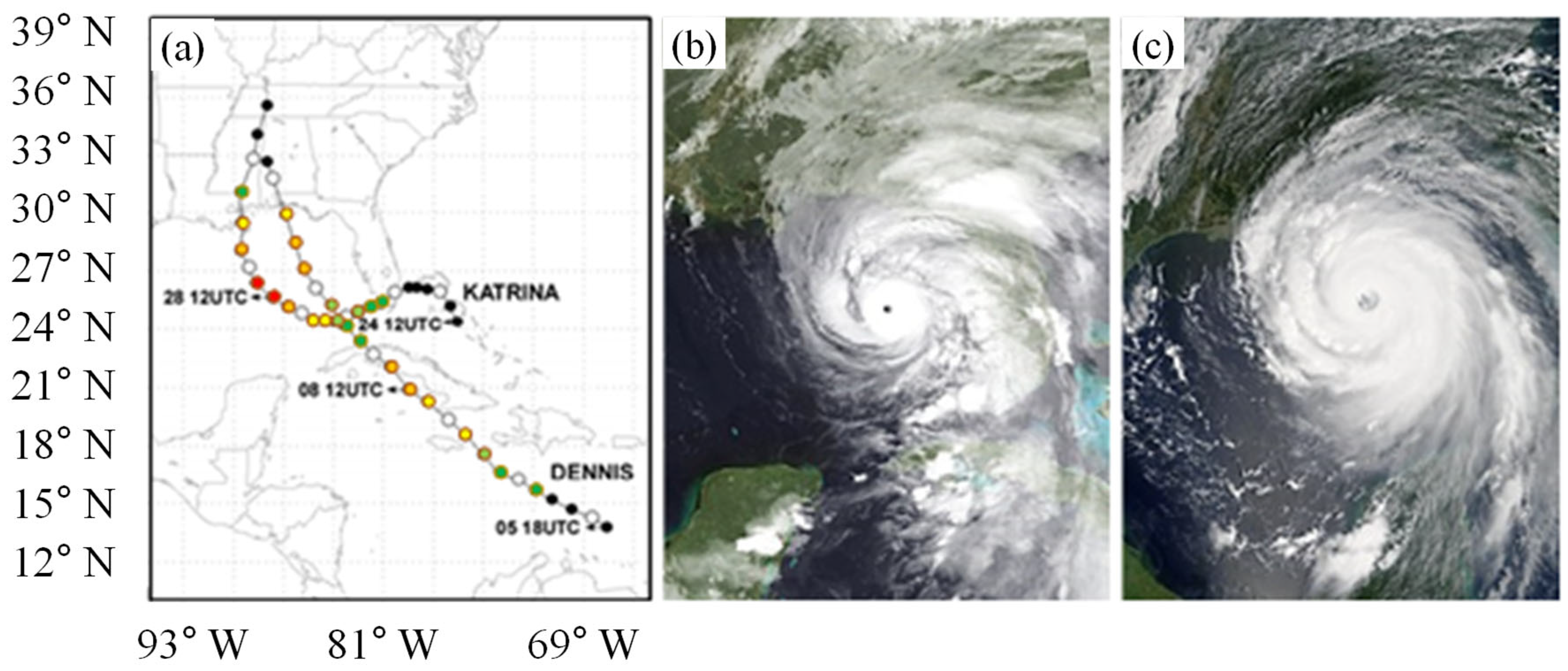
2.1. Brief Description of Hurricanes Katrina and Dennis (2005)

Data for Hurricanes Dennis and Katrina (Figure 1), which posed a severe threat to human life and caused billions of dollars’ worth of damage, were used to test the model’s ability to make predictions regarding intensity near landfall.

Hurricane Dennis was a very strong TC that occurred in July 2005 and moved from the Caribbean Sea up to the Gulf of Mexico; a detailed description is given in Beven [28]. On 5 July the hurricane was a tropical storm, but it reached hurricane category 4 at 12:00 UTC on 8 July. The central pressure was 938 hPa and the maximum wind speed was 66.92 m s⁻¹. It then moved north along the ridge of the Atlantic high before heading toward the Florida Peninsula.

Hurricane Katrina was also a very intense TC that caused severe damage. This hurricane lasted from 23 August to 30 August 2005 and had several landfalls; a detailed description is provided by Knabb et al. [29]. The system evolved as a depression over the southeastern Bahamas on 23 August 2005. The depression then intensified into a category 1 hurricane on the southeastern coast of Florida at around 22:30 UTC on 25 August. As this system moved from west to north, values of 902 hPa and 77 m s⁻¹ were recorded at 18:00 UTC on 28 August. Katrina intensified to a category 5 hurricane as it moved across the Gulf of Mexico. It exhibited category 3 intensity near the mouth of the Pearl River at the Louisiana/Mississippi border at 11:10 UTC on 29 August.

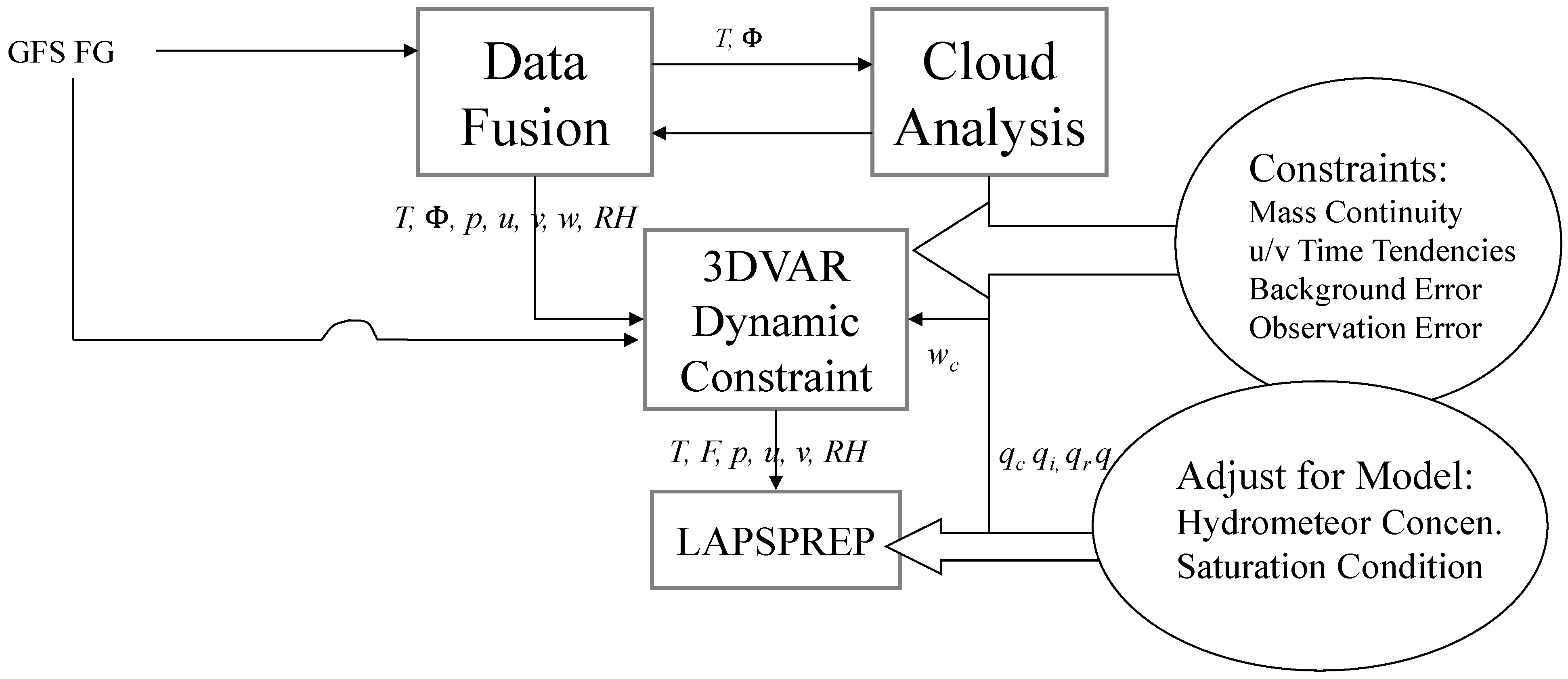
2.2. Hurricane Local Analysis and Prediction System

The tropical cyclone forecasts used in this study were performed using the Hurricane Research System/Hurricane Local Analysis Prediction System (HRS/HLAPS) hybrid model. The HRS was initialized using the HLAPS, as shown in Figure 2. The HLAPS is a hurricane version of diagnostic tool widely used for short-range storm forecasting through wet atmospheric simulations; it eliminates the model spin-up problem and exhibits high computational efficiency [30]. The original LAPS has often been utilized quite successfully for very short-range forecasts of severe weather, such as strong wind and precipitation [31,32,33,34,35,36,37,38]. In this one-way hybrid system, the HLAPS was used to analyze the model first-guess as a “meteorological assimilation system”. A wide range of observational datasets, such as surface observations, wind, temperature radio-sounding profiles, satellite data, and automated aircraft observations (Figure 3), were used in this study.

The following three steps were generally performed in the HLAPS (Figure 2): (1) a two-dimensional (2D) terrestrial analysis and 3D analysis of temperature (T), geopotential height ($\Phi$), wind components (u, v, $\omega$), relative humidity (RH), cloud water (qc), cloud ice (qi), cloud rainwater (qr), and cloud snow (qs); (2) diagnosis of dynamic constraints using the minimum cost function at all grid points following Equation (1) and (3) adjustment of hydrometer concentrations to a saturation condition.

$$\min {\left(X-X^b\right)}^T{B}^{-1}(X-X^b)+{\left(HX-Y^b\right)}^T{O}^{-1}\times (HX-Y^b)+\mathrm{P}$$

(1)

where $X^b$ is the background, $X$ is the analysis result for this “variational sequence”, $Y^b$ is the observation, $H$ is the mapping of the grid space to the observation location, and P is a balancing term added to the analysis. $\mathrm{The} \mathrm{matrics} \mathrm{of} B$ and $O$ are the error covariances for the background and observations, respectively. The cyclostrophic term was adjusted to match the gradient wind slope in the HLAPS, thereby enhancing the geopotential height and temperature perturbation accuracy for the hurricane simulations.

Observation data obtained by NOAA aircraft were also used in this study, i.e., actual observation data from a Hurricane P3 aircraft. The type of data collected differed slightly depending on the aircraft flying time. Figure 3 shows the distribution of all types of data collected for Hurricanes Dennis and Katrina. Figure 3a shows Hurricane Dennis, in which radial velocity was observed within a 2 h window from 21:00 on 5 July 2005. Figure 3b shows the distribution of the observed data in the case of Hurricane Katrina; the data were collected from dropsondes dropped from an aircraft within a 2 h window from 18:00 on 27 August 2005. These observation data were assimilated into the initial field of the model.

2.3. Hurricane Research System

The HRS model is a research version of the Hurricane Weather Research and Forecasting (HWRF) model developed through a collaboration involving with the participation of a number of university scientists and international collaborators [38,39,40].

A non-hydrostatic mesoscale model with a dynamic solver was used [39] with a horizontal Arakawa E-grid and sigma-pressure hybrid vertical coordinates. The HRS parameters used in this study, as shown in

Table 1. Summary of the HRS/HLAPS simulations used in this study.

Category	Description
Grid dimensions	309 × 317	133 × 157
Horizontal-grid increments	19.8 km	6.6 km
Vertical levels	41, top at 50 hPa
Physical parameterization
Thermodynamics	Ferrier (new Eta) microphysics
Radiation parameterization	RRTM longwave and Dudhia shortwave scheme
Cumulus parameterization	Simplified Arakawa–Schubert (SAS) scheme
PBL parameterization	Mellor–Yamada–Janjic TKE scheme
Initial conditions	Hurricane Local Analysis and Prediction System
Lateral boundary conditions	Global Forecasting System

, were in part based on the Ferrier (“new Eta”) microphysical method [41]; this was used for microphysical parameterization, while the Simplified Arakawa–Schubert (SAS) method [42] was used for cumulus parameterization. The Mellor–Yamada–Janjic scheme was adopted for the planetary boundary layer (PBL) process [43]. For radiation, the Rapid Radiative Transfer Model (RRTM) [44] and Dudhia methods [45] were used.

The model was designed to cover North Atlantic Ocean regions with a twice-nested 6.6 km grid. A moving two-way interactive nested grid technique was used to track the vortex with high computational cost efficiency [39,40,46]. The grid dimensions in Domains 1 and 2 were 309 × 317 and 133 × 157, respectively. All domains had 41 vertical layers between the top 50 hPa and the Earth’s surface. Finally, for a soil layer divided into 16 elevation types, and soil utilization divided into 24 types, US Geological Survey data with a 30-s resolution were used. The convective initial condition was taken from the HLAPS mentioned in the previous section. The lateral- and lower-boundary conditions were updated every 6 h based on the Global Forecasting System taken from the National Center of Environmental Prediction.

2.4. Validation Data

For data validation, the absolute values of TC intensity were compared between the observed and simulated data. The best-analyzed observation (Best) of the National Hurricane Center (NHC; Rogers et al. [38]) was used for the observed mean sea level pressure and maximum wind speed for Hurricanes Dennis and Katrina. Track error was calculated using the great-circle distance between the forecasted hurricane position and the best track position, as follows:

$$r{ \cos }^{-1} \left[\cos a \cos b\cos \left(x-y\right)+\sin a \sin b\right]$$

(2)

where $r$ represents the Earth’s radius, $a$ and b indicate the latitude, and x and y indicate the longitude.

3. Results

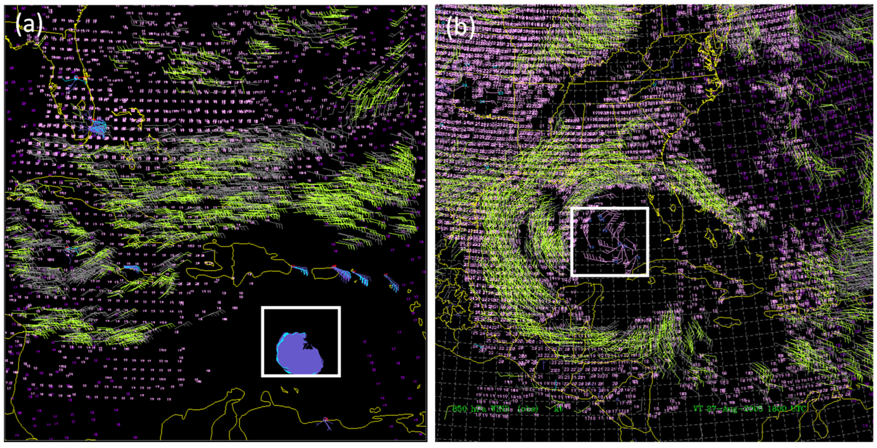
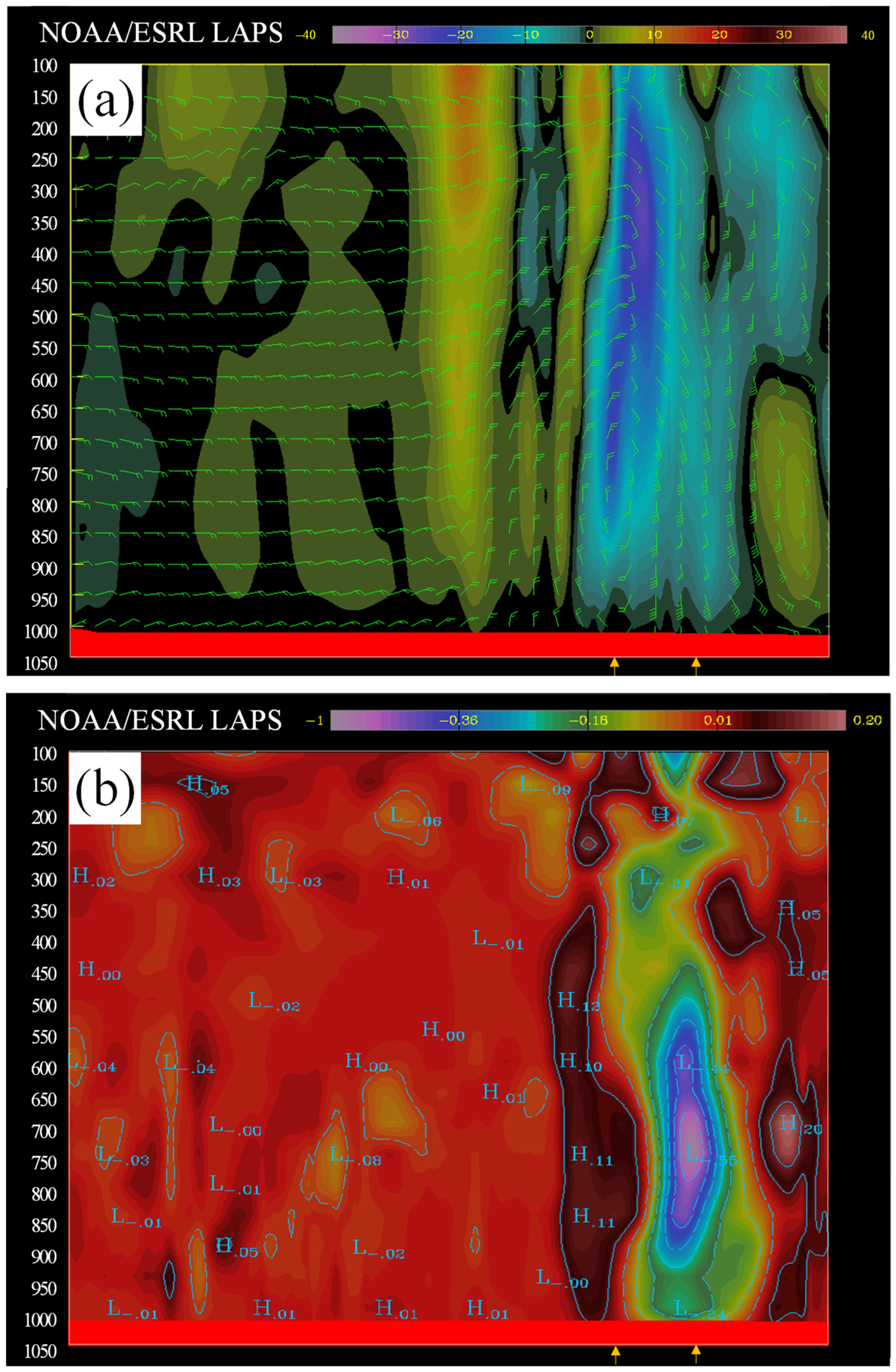
3.1. Model Initialization

Figure 4 and Figure 5 show the initial state assimilated with the HLAPS for the two hurricane cases. The results shown in these figures were compared with the vertical and horizontal structures of the hurricanes after the DA. Figure 4a shows the vertical features of Hurricane Dennis’s circulation in a storm stage. Here, the most important consideration was whether the Doppler radar and dropsonde winds were able to correct for the surrounding field in the HLAPS. The results show Storm Dennis up to the upper troposphere. Updrafts with negative omega were observed around the storm, and downdrafts with positive omega were identified. These vertical circulations represent the growing storm. Figure 4b shows the difference in geopotential height perturbations between the background and analysis fields after assimilation with the HLAPS. When the static equation was combined with the gas state equation, the geopotential height was proportional to the temperature. Thus, the storm warmed up to a maximum of 0.7 °C near 750–850 hPa. The dashed lines in the geopotential height perturbation differences were identified as a negative value of 0.1 m.

The horizontal structure distribution of Hurricane Katrina, in terms of wind speed and direction, is presented in Figure 5. The analyzed winds (Figure 5c,d) were well-balanced based on the three-dimensional DA, and the calm area also shown at the center of the hurricane differed according to whether the flux balance analysis was properly applied by comparing the satellite (Figure 5a) and radar observed images (Figure 5b). The intensified eyewall of the hurricane is shown in the observed images. Regarding the simulated wind field, the strong wind zone (hatched lines) over the eyewall region is longer in Figure 5d compared to Figure 5c. The HLAPS model showed significant improvements in wind speed predictions in most pressure layers compared to the background field without the use of the HLAPS. This was particularly evident at high altitudes, and in all layers below 500 hPa (not shown). Overall, the improvement in wind speed prediction accuracy was approximately 6–8%, having a sufficiently direct impact on vorticity predictions. In summary, the hurricane structure was more accurately represented using well-balanced data.

3.2. Impact of Data Assimilation

To investigate the impact of observations on hurricane predictions, various hurricane simulations were conducted. Figure 6 and

Table 2. Summary of the forecast track and intensity errors of the Global Forecasting System (GFS), Hurricane Research System (HRS), and HRS coupled with the Hurricane Local Analysis Prediction System (HRS/HLAPS) models for Hurricanes Dennis and Katrina relative to the best-analyzed observation (Best). Bold italics indicate the smallest values.

TC	Variable	0 h	6 h	12 h	18 h	24 h	48 h	72 h
Dennis
GFS	Dist (km) MLSP (hPa) MWS (knots)	19.46 24.67 25.05	58.25 38.00 1.65	59.29 39.67 −15.50	69.51 46.34 −23.85	88.97 49.00 −57.25	89.17 37.00 −23.85	88.72 48.80 −66.70
HRS	Dist (km) MLSP (hPa) MWS (knots)	19.46 9.00 −7.25	94.47 25.00 −22.75	75.62 30.70 −46.70	117.53 31.60 −43.30	200.70 36.90 −79.45	204.58 26.30 −57.25	239.33 34.20 −67.25
HRS/HLAPS	Dist (km) MLSP (hPa) MWS (knots)	5.56 8.00 −7.00	65.11 16.50 −1.65	63.03 25.30 −28.90	100.77 34.60 −29.00	140.95 40.60 −51.10	203.56 29.30 −39.45	142.20 15.70 −23.95
Katrina
GFS	Dist (km) MLSP (hPa) MWS (knots)	27.38 54.50 −37.60	53.20 45.50 −38.60	8.40 39.00 −38.40	42.53 50.00 −64.60	22.44 70.50 −83.35	190.78 40.50 −48.35	349.35 14.00 27.80
HRS	Dist (km) MLSP (hPa) MWS (knots)	23.67 33.50 −33.40	14.10 9.50 −33.90	47.60 15.50 −11.10	63.47 24.00 −37.10	96.98 29.00 −53.35	131.93 −22.00 40.00	170.73 −24.50 26.70
HRS/HLAPS	Dist (km) MLSP (hPa) MWS (knots)	14.45 1.00 −12.30	33.79 14.00 −13.80	37.52 20.00 −7.25	53.01 31.00 −36.10	97.93 32.00 −51.15	49.36 −3.00 11.65	98.57 −1.50 0.00

compare the tracks and changes in intensity among three different TC simulations, i.e., the HLAPS-initialized HRS (HRS/HLAPS, yellow lines with symbols in Figure 6), the HRS without the HLAPS initialization (HRS, green lines with symbols in Figure 6), and the background first guess (i.e., GFS, blue lines with symbols in Figure 6). The track and intensity errors for GFS, HRS, and HRS/HLAPS shown in Figure 6 are summarized in Table 2.

Both hurricanes largely followed the actual best track. The predicted path was quite similar to that of Hurricane Dennis in the early phase. However, it deviated slightly from the predicted TC track after 12 h. Moreover, the track prediction error of HRS/HLAPS was larger than that of the GFS after 24 h. The HRS/HLAPS predictions were more consistent with the actual best track for the predicted track pattern over time than those of GFS and HRS (Figure 6a). For Hurricane Katrina, track prediction was considerably improved compared to those of Best and GFS, with <100 km of track error during the 72-h lead time (Figure 6b). This error was comparable to that of the 126.7 km obtained using European Centre for Medium-Range Weather Forecasts (ECMWF) data, which are recognized as the most accurate data currently available.

Figure 6c, d shows the intensity changes obtained by HRS/HLAPS compared to those of Best, GFS, and HRS. The TC intensity for Hurricane Dennis was underestimated for up to 42 h. However, as the hurricane passed across Cuba and reached the Caribbean Sea, the TC intensity changes were well-captured by the model after 48 h. The increasing trend in the minimum sea level pressure (MSLP) and maximum wind speed were relatively well simulated with a 48-h lead time, with higher intensity compared to GFS. The HRS/HLAPS model provided more accurate results than the GFS model in terms of the prediction of both path and intensity for Hurricane Katrina, after 24 h and for up to 72 h. It was predicted that Hurricane Katrina would be well-developed, with a minimum pressure of around 935 hPa around the time of landfall (after 24 h), similar to the results obtained with Best. The maximum wind speed was 57.14 ms⁻¹. Compared to the best track data, accuracy was improved by 59.11% by the HRS/HLAPS simulation (Figure 6d). Figure 7 is the horizontal distribution of the precipitation prediction and HRS and HRS/HLAPS with a 6 h lead time compared to the satellite composite imagery (Figure 7a). The HRS/HLAPS model showed better-organized spiral bands than the HRS model. White lines are drawn to identify the eyewall, the connecting band, the secondary band, and the principal bands. All bands presented in the simulated precipitation were taken from the HRS/HLAPS model.

4. Discussion

TC evolution in numerical models is highly dependent on initial and boundary conditions; it is difficult to compare the predictability of TC modeling. In this section, the TC results obtained from the HRS/HLAPS simulations are discussed by comparing the GFS boundary conditions for the intensification of Hurricanes Dennis and Katrina. Figure 8, Figure 9 to Figure 10 show cross-sections of the TC structure according to the GFS and HRS/HLAPS models, with 24 and 48 h lead times. The left and right panels in Figure 8, Figure 9 and Figure 10 indicate the results of Hurricane Dennis and Katrina, respectively.

The cross-sections indicate that the TC intensification was greater with a 48-h lead time compared to that of a 24 h lead time, as shown in Figure 6. At a 24 h lead time, Hurricane Dennis was under development and grew slightly by a 48-h lead time (Figure 8a–d). Hurricane Katrina has already developed and extended to full altitudes between 24 h and 48 h (Figure 8e–h). The cross-section of the equivalent potential temperature and radial winds in the 48-h forecast field revealed weakened subsidence (Figure 9d) and a decrease in the inward flows (Figure 10d), respectively. This was conducted as vortices in the lower layer decreased due to increased roughness and decreased moisture in the lower layer (Figure 8d). The latent heat decreased as Hurricane Dennis approached Cuba (Figure 6). Lower boundary forcing had a greater effect on the TC intensity than the initial and lateral boundary forcing. Conversely, Hurricane Katrina grew stronger and the vortex at its center strengthened, while the warm core became more pronounced. The forecast shows reasonable accuracy in terms of TC track and intensity (Figure 6).

5. Conclusions

This study examined the impact of assimilating airborne observations into a mesoscale model for predicting the track and intensity of two severe hurricanes (Katrina and Dennis) that affected southern parts of the United States in 2005. HLAPS was developed by modifying the general LAPS to incorporate and balance hurricane extreme observations. It was used for the initialization of HRS (HRS/HLAPS), and simulations were performed without spin-up problems and showed fast computation speed. HLAPS analyzed dropsonde observations and radar data collected by NOAA aircraft within the initial 2 h of the lifespan of hurricanes; the data were then examined using the HRS model for long-term TC forecasting. HRS/HLAPS used 19.8 km domain data, which was refined to a 6.6 km domain.

Our experiments show that the tracks simulated by the different models (small errors between simulations and the Best) differed very slightly. However, there was a large difference in the simulated intensity (large errors between the simulations and the Best). The HRS/HLAPS model showed the best performance overall of the lead time, with respect to the GFS and HRS models, with the smallest errors. The predicted path in HRS/HLAPS was considerably improved compared to those of Best and GFS, with less than 100 km of track error during the 72-h lead time. The results of the HRS/HLAPS model show that the maximum duration of the effect of intensification and the TC structure assimilated with the observed data was between 6 and 12 h, similar to the findings of Zhang et al. [26]. However, unlike Zhang et al., we had valid forecast data from 0 to 4 h, i.e., prior to 8 h [26]. Although the two hurricanes had different life cycles, both showed that the TC intensity simulated by HRS/HLAPS was relatively higher than those in GFS and HRS because of the vertical wind shear, the heat content of the sea surface, and sufficient water vapor supply (and retention thereof in the lower layer). The simulated horizontal and vertical structures of both hurricanes were similar to the observations but differed from those seen in the global analysis with coarse-resolution data. The well-organized spiral structure of convection bands in the HRS/HLAPS model was also captured, particularly within the 6 h spin-up time, due to vertical wind shear and water vapor trapped in the lower atmosphere. We also identified that the development of the TCs was significantly affected by the boundary forcing after 24 h.

Our results may aid long-term operational forecasts, although the underestimation of hurricane intensity between 12 and 36 h needs to be investigated. To improve this approach, more research is required on the potential of hurricane observations to improve mesoscale models [47], for example, by improving grid spacing and physical parameterization for more TC cases. Additionally, recently serviced satellite images [48] could be applied in studies focusing on environmental flow associated with TCs.

References

1. Frank, W.M.; Young, G.S. The interannual variability of tropical cyclones. Mon. Weather Rev. 2007, 135, 3587–3598. [Google Scholar] [CrossRef]
2. Pielke, J.R.A.; Gratz, J.; Landsea, C.W.; Collins, D.; Saunders, M.A.; Musulin, R. Normalized hurricane damage in the United States: 1900–2005. Nat. Hazards Rev. 2008, 9, 30–42. [Google Scholar] [CrossRef]
3. Weinkle, J.; Maue, R.; Pielke, J.R. Historical global tropical cyclone landfalls. J. Clim. 2012, 25, 4729–4735. [Google Scholar] [CrossRef]
4. Done, J.M.; Simmons, K.M.; Czajkowski, J. Relationship between residential losses and hurricane winds: Role of the Florida building code. ASCE-ASME J. Risk Uncertain. Eng. Syst. A Civ. Eng. 2018, 4, 04018001. [Google Scholar] [CrossRef]
5. Munich, R. Topics Geo Natural Catastrophes 2017: Analyses, Assessments, Positions. Available online: www.readkong.com/page/a-stormy-year-topics-geo-natural-catastrophes-2017-6234005 (accessed on 16 August 2022).
6. Liu, K.S.; Chang, J.C.L. Recent increase in extreme intensity of tropical cyclones making landfall in South Korea. Clim. Dyn. 2020, 55, 1059–1074. [Google Scholar] [CrossRef]
7. Elsberry, R.L.; Marks, F.D. The Hurricane Landfall Workshop summary. Bull. Am. Meteorol. Soc. 1999, 80, 683–685. [Google Scholar]
8. Aberson, S.D.; Etherton, B.J. Targeting and data assimilation studies during Hurricane Humberto (2001). J. Atmos. Sci. 2006, 63, 175–186. [Google Scholar] [CrossRef]
9. Davis, C.; Wang, W.; Chen, S.; Chen, Y.; Corbosiero, K.; DeMaria, M.; Dudhia, J.; Holland, G.; Klenmp, J.; Michalakes, J.; et al. Prediction of landfalling hurricanes with the advanced hurricane WRF model. Mon. Weather Rev. 2008, 136, 1990–2005. [Google Scholar] [CrossRef]
10. Zhang, F.; Sippel, J.A. Effects of moist convection on hurricane predictability. J. Atmos. Sci. 2009, 66, 1944–1961. [Google Scholar] [CrossRef]
11. Pattanayak, S.; Mohanty, U.C.; Osuri, K.K. Impact of Parameterization of Physical Processes on Simulation of Track and Intensity of Tropical Cyclone Nargis (2008) with WRF-NMM Model. Sci. World J. 2012, 2012, 671437. [Google Scholar] [CrossRef]
12. Zhang, Y.; Meng, Z.; Zhang, F.; Weng, Y. Predictability of tropical cyclone intensity evaluated through 5-yr forecasts with a convection-permitting regional-scale model in the Atlantic Basin. Weather Forecast. 2014, 29, 1003–1023. [Google Scholar] [CrossRef]
13. Lu, X.; Wang, X.; Li, Y.; Tong, M.; Ma, X. GSI-based ensemble-variational hybrid data assimilation for HWRF for hurricane initialization and prediction: Impact of various error covariances for airborne radar observation assimilation. Q. J. R. Meteorol. Soc. 2017, 143, 223–239. [Google Scholar] [CrossRef]
14. Zhu, P.; Zhu, Z.; Gopalakrishnan, S.; Black, R.; Marks, F.D.; Tallapragada, V.; Zhang, J.A.; Zhang, X.; Gao, C. Impact of subgrid-scale processes on eyewall replacement cycle of tropical cyclones in HWRF system. Geophys. Res. Lett. 2015, 42, 10,027–10,036. [Google Scholar] [CrossRef]
15. Pu, Z.; Li, X.; Sun, J. Impact of airborne Doppler radar data assimilation on the numerical simulation of intensity changes of Hurricane Dennis near a landfall. J. Atmos. Sci. 2009, 66, 3351–3365. [Google Scholar] [CrossRef]
16. Weng, Y.; Zhang, F. Assimilating airborne Dopplr radar observations with ensemble Kalman filter for convection-permitting hurricane initialization and prediction: Katrina (2005). Mon. Weather Rev. 2012, 140, 841–859. [Google Scholar] [CrossRef]
17. Aksoy, A.; Lorsolo, S.; Vukicevic, T.; Sellwood, K.J.; Aberson, S.D.; Zhang, F. The HWRF Hurricane Ensemble Data Assimilation System (HEDAS) for high-resolution data: The impact of airborne Doppler radar observations in an OSSE. Mon. Weather Rev. 2012, 140, 1843–1862. [Google Scholar] [CrossRef]
18. Du, N.; Xue, M.; Zhao, K.; Min, J. Impact of assimilating airborne Doppler radar velocity data using the ARPS 3DVAR on the analysis and prediction of Hurricane Ike (2008). J. Geophys. Res. 2012, 117, D18113. [Google Scholar] [CrossRef]
19. Tong, M.; Sippel, J.A.; Tallagragada, V.; Liu, E.; Kieu, C.; Kwon, I.H.; Wang, W.; Liu, Q.; Ling, Y.; Zhang, B. Impact of Assimilating Aircraft Reconnaissance Observations on Tropical Cyclone Initialization and Prediction Using Operational HWRF and GSI Ensemble-Variational Hybrid Data Assimilation. Mon. Weather Rev. 2018, 146, 4155–4177. [Google Scholar] [CrossRef]
20. Elsberry, R.L.; Hendricks, E.A.; Velden, C.S.; Bell, M.M.; Peng, M.; Casas, E.; Zhao, Q. Demonstration with special TCI-15 datasets of potential impacts of new-generation satellite atmospheric motion vectors on Navy regional and global models. Weather Forecast. 2018, 33, 1617–1637. [Google Scholar] [CrossRef]
21. Minanmide, M.; Zhang, F. Assimilation of all-sky infrared radiances from Himawari-8 and impacts of moisture and hydrometer initialization on convection-permitting tropical cyclone prediction. Mon. Weather Rev. 2018, 146, 3241–3258. [Google Scholar] [CrossRef]
22. Sawada, M.; Ma, Z.; Mehra, A.; Tallapragada, V.; Oyama, R.; Shimoji, K. Assimilation of himawari-8 rapid-scan atmospheric motion vectors on tropical cyclone in HWRF system. Atmosphere 2020, 11, 601. [Google Scholar] [CrossRef]
23. Tian, X.; Zou, X. A comprehensive 4D-Var vortex initialization using a nonhydrostatic axisymmetric TC model with convection accounted for. Tellus A Dyn. Meteorol. Oceanogr. 2019, 71, 1653138. [Google Scholar] [CrossRef]
24. Zhang, S.; Pu, Z. Numerical simulation of rapid weakening of Hurricane Joaquin with assimilation of high-definition sounding system dropsondes during the tropical cyclone intensity experiment: Comparison of three- and four-dimensional ensemble-variational data assimilation. Weather Forecast. 2019, 34, 521–538. [Google Scholar] [CrossRef]
25. Chang, Y.P.; Yang, S.C.; Lin, K.J.; Lien, G.Y.; Wu, C.M. Osse assessment of underwater glider arrays to improve ocean model initialization for tropical cyclone prediction. J. Atmos. Sci. 2010, 77, 467–487. [Google Scholar]
26. Dong, J.; Xue, M. Assimilation of radial velocity and reflectivity data from coastal WSR-88D radars using an ensemble Kalman filter for the analysis and forecast of landfalling hurricane Ike (2008). Q. J. R. Meteorol. Soc. 2013, 139, 467–487. [Google Scholar] [CrossRef]
27. Zhang, F.; Weng, Y.; Gamache, J.F.; Marks, F.D. Performance of convection-permitting hurricane initialization and prediction during 2008–2010 with ensemble data assimilation of inner-core airborne Doppler radar observations. Geophys. Res. Lett. 2011, 38, L15810. [Google Scholar] [CrossRef]
28. Beven, J. Tropical Cyclone Report Hurricane Dennis 4–13 July 2005. Available online: https://www.nhc.noaa.gov/data/tcr/AL042005_Dennis.pdf (accessed on 16 August 2022).
29. Knabb, R.D.; Rhome, J.R.; Brown, D.P. Tropical Cyclone Report Hurricane Katrina 23–30 August 2005. Available online: https://www.nhc.noaa.gov/data/tcr/AL122005_Katrina.pdf (accessed on 16 August 2022).
30. Snook, J.S.; Cram, J.M. Schmidt JM. LAPS/RAMS. A nonhydrostatic mesoscale numerical modeling system configured for operational use. Tellus A Dyn. Meteorol. Oceanogr. 1995, 47, 864–875. [Google Scholar] [CrossRef]
31. Jian, G.J.; McGinley, J.A. Evaluation of a short-range forecast system on quantitative precipitation forecasts associated with tropical cyclones of 2003 near Taiwan. J. Meteorol. Soc. Jpn. 2005, 83, 657–681. [Google Scholar] [CrossRef]
32. Gregow, E.; Pressi, A.; Mäkelä, A.; Saltikoff, E. Improving the precipitation accumulation analysis using lightning measurements and different integration periods. Hydrol. Earth Syst. Sci. 2017, 21, 267–279. [Google Scholar] [CrossRef]
33. Albers, S.C.; McGinley, J.A.; Birkenheuer, D.L.; Smart, J.R. The Local Analysis and Prediction System (LAPS): Analyses of Clouds, Precipitation, and Temperature. Weather Forecast. 1996, 11, 273–287. [Google Scholar] [CrossRef]
34. Xie, Y.; Koch, S.; McGinley, J.; Albers, S.; Beringer, P.; Wolfson, M.; Chang, M. A space-time multiscale analysis system: A sequential variational analysis approach. Mon. Weather Rev. 2011, 139, 1224–1240. [Google Scholar] [CrossRef]
35. Kim, O.Y.; Lu, C.; McGinley, J.A.; Albers, S.C.; Oh, J.H. Experiments of LAPS wind and temperature analysis with background error statistics obtained using ensemble methods. Atmos. Res. 2013, 122, 250–269. [Google Scholar] [CrossRef]
36. Jiang, H.; Albers, S.; Xie, Y.; Toth, Z.; Jankove, I.; Scotten, M.; Picca, J.; Stumpf, G.; Kingfield, D.; Birkenheuer, D. Real-Time Applications of the Variational Version of the Local Analysis and Prediction System (vLAPS). Bull. Am. Meteorol. Soc. 2016, 80, 683–685. [Google Scholar] [CrossRef]
37. McGinley, J.A.; Albers, S.C.; Stamus, P.A. Validation of a Composite Convective Index as Defined by a Real-Time Local Analysis System. Weather Forecast. 1991, 6, 337–356. [Google Scholar] [CrossRef]
38. Rogers, R.; Aberson, S.; Aksoy, A.; Annane, B.; Black, M.; Cione, J.; Dorst, N.; Dunion, J.; Gamache, J.; Goldenberg, S.; et al. NOAA’S Hurricane Intensity Forecasting Experiment: A Progress Report. Bull. Am. Meteorol. Soc. 2013, 94, 859–882. [Google Scholar] [CrossRef]
39. Gopalakrishnan, S.; Liu, Q.; Marchok, T.; Sheinin, D.; Surgi, N.; Tuleya, R.; Yablonski, R.; Zhang, X. Hurricane Weather Research and Forecasting (HWRF) Scientific Documentation. Available online: https://dtcenter.org/sites/default/files/community-code/hwrf/docs/scientific_documents/HWRFv4.0a_ScientificDoc.pdf (accessed on 16 August 2022).
40. Gopalakrishnan, S.G.; Bacon, D.P.; Ahmad, N.N.; Boybeyi, Z.; Dunn, T.J.; Hall, M.S.; Jin, Y.; Lee, P.C.S.; Mays, D.E.; Madala, R.V.; et al. An operational multiscale hurricane forecasting system. Mon. Weather Rev. 2002, 130, 1830–1847. [Google Scholar] [CrossRef]
41. Ferrier, B.S.; Tao, W.-K.; Simpson, J. A double-moment multiplephase four-class bulk ice scheme. Part II: Simulations of convective storms in different large-scale environments and comparisons with other bulk parameterizations. J. Atmos. Sci. 1995, 52, 1001–1033. [Google Scholar] [CrossRef]
42. Troen, I.B.; Mahrt, L. A simple model of the atmospheric boundary layer sensitivity to surface evaporation. Bound.-Layer Meteorol. 1986, 37, 129–148. [Google Scholar] [CrossRef]
43. Janjić, Z.I. Nonsingular Implementation of the Mellor-Yamada Level 2.5 Scheme in the NCEP Meso Model; Office Note No. 437; National Centers for Environmental Prediction: Washington, DC, USA, 2001; p. 61.
44. Mlawer, E.J.; Taubman, S.J.; Brown, P.D.; Iacono, M.J. Clough SA. Radiative transfer for inhomogeneous atmospheres: RRTM, a validated correlated-k model for the longwave. J. Geophys. Res. 1997, 102, 16663–16682. [Google Scholar] [CrossRef]
45. Dudhia, J. Numerical study of convection observed during the winter monsoon experiment using a mesoscale two-dimensional model. J. Atmos. Sci. 1989, 46, 3077–3107. [Google Scholar] [CrossRef]
46. Phillips, N.A.; Shukla, J. On the strategy of combining coarse and fine grid meshes in numerical weather prediction. J. Appl. Meteorol. Climatol. 1973, 12, 763–770. [Google Scholar] [CrossRef]
47. Bielli, S.; Barthe, C.; Bousquet, O.; Tulet, P.; Pianezze, J. The Effect of Atmosphere-Ocean Coupling on the Structure and Intensity of Tropical Cyclone Bejisa in the Southwest Indian Ocean. Atmosphere 2021, 12, 688. [Google Scholar] [CrossRef]
48. Manaster, A.; Ricciardulli, L.; Meissner, T. Tropical Cyclone Winds from WindSat, AMSR2, and SMAP: Comparison with the HWRF Model. Remote Sens. 2021, 13, 2347. [Google Scholar] [CrossRef]
Figure 1. The track and intensity of Hurricanes Dennis and Katrina. The symbols shown in (a) were plotted every 6 h and the colors denote storm intensity categories on the Saffir–Simpson scale (category 1, green; category 2, light green; category 3, yellow; category 4, dark orange; category 5, red). (b) and (c) are images of Dennis and Katrina at their peak intensity on 10 July and 28 August 2005, respectively.
Atmosphere 13 01302 g001
Figure 2. Schematic diagram of the Hurricane Local Analysis Prediction System (HLAPS) used in this study. T, Φ , u, v, ω , RH, qc, q, qr, and qs indicate temperature, geopotential height, wind components, relative humidity, cloud water, cloud ice, cloud rainwater, and cloud snow, respectively.
Atmosphere 13 01302 g002
Figure 3. Observation data for Hurricanes (a) Dennis and (b) Katrina used in this study. The pink, red, green, and blue colors indicate the Geostationary Operational Environmental Satellite/Polar Operational Environmental Satellites soundings, Aircraft Communications Addressing and Reporting System (ACARS) data, winds from the Cloud Motion Vector Sensor (CMVS), and Doppler radar data, respectively. The outer and inner boxes indicate the mother and nested domain in the Hurricane Research System coupled with the Hurricane Local Analysis Prediction System (HRS/HLAPS), respectively.
Atmosphere 13 01302 g003
Figure 4. Cross-section of (a) wind (knots) and omega (μbar s−1) values, and (b) geopotential height perturbation differences (0.1 m) between the background and the Hurricane Local Analysis Prediction System (HLAPS) simulation of Hurricane Dennis. Yellow arrows indicate the cyclone center and wall.
Atmosphere 13 01302 g004
Figure 5. Horizontal distribution of the observed (upper panels) and analyzed (lower panels) Hurricane Katrina. (a,b) are the satellite visible (19:25 August 2017) and reflectivity imagery (18:15 to 18:25 27 August), respectively. (c,d) are the analyzed wind speed (shaded area) and direction (wind barbs) under imbalanced and balanced conditions obtained for 18:00 27 August using he Hurricane Local Analysis Prediction System (HLAPS), respectively. Blue (white) to red (bright white) color indicates the strengthened wind speed (intensified cloudiness). Dashed lines in (d) present the intensified wind-speed zone compared to those in (c).
Atmosphere 13 01302 g005
Figure 6. The 72-h forecast track (a,b) and intensity (c,d) for Hurricane Dennis (a,c) and Hurricane Katrina (b,d), according to the best-analyzed observation (Best), Global Forecasting System (GFS), Hurricane Research System (HRS), and HRS coupled with the Hurricane Local Analysis Prediction System (HRS/HLAPS). The black, blue, green, and yellow colors represent the Best, GFS, HRS, and HRS/HLAPS models, respectively. Symbols are plotted every 6 h.
Atmosphere 13 01302 g006
Figure 7. The total precipitation (mm) determined based on (a) satellite composite imagery (courtesy of Atlantic Oceanographic and Meteorological Laboratory), (b) the Hurricane Research System (HRS) and (c) HRS coupled with the Hurricane Local Analysis Prediction System (HRS/HLAPS) models at the 6 h forecast time for Hurricane Katrina. White lines indicate the precipitation echo patterns with a threshold of 3 kg/m2.
Atmosphere 13 01302 g007
Figure 8. Cross-sections showing the relative vorticity (s−1) of the TC according to (a,c,e,g) 24 and (b,d,f,h) 48 h forecasts taken from the GFS (upper panels) and HRS/HLAPS (lower panels). The left and right panels are for Hurricanes Dennis and Katrina, respectively.
Atmosphere 13 01302 g008
Figure 9. Cross-sections showing the equivalent potential temperature (K) of the TC according to (a,c,e,g) 24 and (b,d,f,h) 48 h forecasts taken from the GFS (upper panels) and HRS/HLAPS (lower panels). The left and right panels are for Hurricanes Dennis and Katrina, respectively.
Atmosphere 13 01302 g009
Figure 10. Cross-sections showing the radial wind (m s−1) of the TC according to (a,c,e,g) 24 and (b,d,f,h) 48 h forecasts taken from the GFS (upper panels) and HRS/HLAPS (lower panels). The left and right panels are for Hurricanes Dennis and Katrina, respectively.
Atmosphere 13 01302 g010