Sea Surface Temperature and Marine Heat Wave Predictions in the South China Sea: A 3D U-Net Deep Learning Model Integrating Multi-Source Data

Abstract

Accurate sea surface temperature (SST) prediction is vital for disaster prevention, ocean circulation, and climate change. Traditional SST prediction methods, predominantly reliant on time-intensive numerical models, face challenges in terms of speed and efficiency. In this study, we developed a novel deep learning approach using a 3D U-Net structure with multi-source data to forecast SST in the South China Sea (SCS). SST, sea surface height anomaly (SSHA), and sea surface wind (SSW) were used as input variables. Compared with the convolutional long short-term memory (ConvLSTM) model, the 3D U-Net model achieved more accurate predictions at all lead times (from 1 to 30 days) and performed better in different seasons. Spatially, the 3D U-Net model’s SST predictions exhibited low errors (RMSE < 0.5 °C) and high correlation (R > 0.9) across most of the SCS. The spatially averaged time series of SST, both predicted by the 3D U-Net and observed in 2021, showed remarkable consistency. A noteworthy application of the 3D U-Net model in this research was the successful detection of marine heat wave (MHW) events in the SCS in 2021. The model accurately captured the occurrence frequency, total duration, average duration, and average cumulative intensity of MHW events, aligning closely with the observed data. Sensitive experiments showed that SSHA and SSW have significant impacts on the prediction of the 3D U-Net model, which can improve the accuracy and play different roles in different forecast periods. The combination of the 3D U-Net model with multi-source sea surface variables, not only rapidly predicted SST in the SCS but also presented a novel method for forecasting MHW events, highlighting its significant potential and advantages.

1. Introduction

As an important parameter for oceanic systems, the sea surface temperature (SST) is crucial for exchanging energy, momentum, and moisture between the ocean and the atmosphere [1,2,3]. Changes in SST can affect air–sea interaction, circulation patterns, and precipitation, subsequently influencing a range of weather, oceanic, and climate phenomena [4,5], such as El Niño–Southern Oscillation [6], Indian Ocean Dipole (IOD) [7,8], and coral bleaching [9]. Furthermore, variations in SST are also important for the formation, evolution, and trajectory of tropical cyclones [10,11,12]. Consequently, accurate prediction of SST is essential for detecting oceanic extreme events and enhancing our understanding of ocean and climate change. However, accurate prediction of SST remains challenging, especially in regions with high variability, due to complex dynamic and thermal processes at the air–sea interface, including ocean waves [13], turbulence [14], and radiation fluxes [15].

The South China Sea (SCS), a semi-enclosed marginal sea located in the southeastern part of the Asian continent, plays an important role in global climate patterns due to its location within the Indo-Pacific warm water pool, known for its higher SST [16]. Through various straits, it connects to the Pacific Ocean, the Indian Ocean, and other seas. Due to the unique geographical position of the SCS, combined with the influence of monsoons, a complex circulation system has resulted [17], as illustrated in Figure 1. The variability of SST in the SCS, typically following a southwest–northeast gradient with temperatures rising from north to south, is significantly impacted by this system [18]. The distinct geographical characteristics and complex circulation patterns of the SCS make its SST variations particularly important. For example, a rise in SST can intensify monsoon activity, altering regional precipitation patterns [19]. Additionally, higher SST in the SCS can lead to coral bleaching, impacting the rich biodiversity within and around these waters [9]. Consequently, accurately predicting these SST changes is crucial for understanding regional ocean circulation and the broader effects of climate change. However, this prediction is highly challenging, owing to the significant variations in heat flux, radiation, and wind stress.

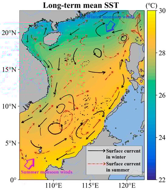
Figure 1. Schematic diagram of the circulation structure in the SCS and the long-term average SST (°C) derived from OISST data from 1 January 1982 to 31 December 2021.

Currently, SST prediction methods are mainly divided into physics-based and data-driven methods. Physics-based models, while offering detailed representations of ocean dynamics, are computationally demanding because they need to account for complex dynamic and physical processes in the ocean [20,21,22]. In contrast, data-driven statistical methods and machine learning models are gradually being applied to predicting SST by accumulating oceanic data and technological advancements. These methods, including Markov models [23,24], canonical correlation analysis [25], linear regression [26], and support vector machine (SVM) [27], use historical data to discern patterns and relationships. While these approaches are computationally more efficient, they generally lack the complexity of their numerical counterparts, focusing primarily on pattern recognition and statistical inference. This simplicity limits their effectiveness in capturing the nonlinear dynamics of ocean processes, often resulting in lower predictive accuracy than numerical models.

Due to the powerful nonlinear feature extraction capabilities, deep learning models developed through advancements in artificial intelligence technology have been increasingly applied in predicting SST. Various models such as back propagation neural networks (BPNN) [28], wavelet neural networks (WNN) [29], convolutional neural networks (CNN) [30], and long short-term memory (LSTM) [31,32] have demonstrated efficacy in predicting SST and its related phenomena. For example, Xiao et al. [33] used an AdaBoost model combined with LSTM to predict SST anomalies (SSTA), outperforming conventional models like support vector regression (SVR) and BPNN in the East China Sea. Furthermore, Yang et al. [34] integrated LSTM with convolutional layers for improved SST prediction accuracy, outperforming traditional SVR and fully connected LSTM methods. Similarly, the U-Net–LSTM model by Taylor and Feng [35] combined 2D convolution with LSTM for monthly mean SST prediction, effectively aiding forecasting phenomena like El Niño. Despite these advancements, most studies, including those in the SCS by Song et al. [36] and Hao et al. [37], have primarily utilized single-variable predictions, overlooking the interplay between different oceanic variables. This approach often limits the physical significance and overall accuracy of the models. Previous studies indicate that multivariable inputs often lead to better forecasting outcomes. Shao et al. [38] established an advanced model with physical information, which combined the multivariate empirical orthogonal functions (MEOF) and Conv1D–LSTM, using sea surface height anomaly (SSHA) and SST for short-term prediction, and considered the correlation between different variables. This model exhibited strong performance in both normal and extreme weather conditions. Recently, Miao et al. [39] also reached similar conclusions. Based on a multivariate CNN model, they used SSTA, wind speeds, and surface current velocity as input variables to predict SSTA, achieving more accurate forecasts.

In summary, while deep learning has significantly enhanced SST prediction capabilities, research specifically focused on the SCS remains limited. Existing models often focus on single-point predictions or individual variables, overlooking the complex interplay among different variables, which can diminish their physical relevance and accuracy. Their forecasting accuracy also requires further improvement. To solve these limitations, a novel deep learning model based on the 3D U-Net architecture is introduced in this study. This model has been designed to effectively capture the intricate correlations between multiple sea surface variables and extract spatiotemporal features. Its application marks a significant advancement in SST prediction for the SCS, potentially enhancing the model’s accuracy and physical relevance. The remaining parts of this study are organized as follows: Section 2 details the various sea surface data of the SCS used in the study and the SST prediction models established. The presentation and evaluation of the results are in Section 3. Section 4 is the summary and discussion of the study.

2. Data and Methods

2.1. Data

This study focuses on the SCS region, specifically between 105° E and 122.5° E longitude and 0° to 23° N latitude, as shown in Figure 1. The Sulu and Celebes Seas are not included to avoid their impact on the prediction and result analysis. Considering previous research conclusions and the quality and accessibility of data from satellite remote sensing, we chose SST, sea surface wind (SSW), and SSHA as our input parameters in this study. These were selected for their demonstrated relevance in predicting SST patterns, as well as for the reliability of the data associated with them.

The SST data used in this study were obtained from the National Oceanic and Atmospheric Administration (NOAA) Daily Optimum Interpolation SST (OISST) version 2.1 dataset [40], with a resolution of 0.25°. The dataset is a composite of multiple SST data sources, filling gaps with optimum interpolation techniques. This dataset encompassed a period from September 1, 1981, to the present.

The SSW data were obtained from the Cross-Calibrated Multi-Platform (CCMP) dataset v2.0 [41], with a resolution of 0.25°. The dataset was composed of eastward SSW (ESSW) and northward SSW (NSSW) from 10 July 1987 to the present, with a temporal resolution of one-fourth of a day.

Lastly, the SSHA data were obtained from the Collecte Localisation Satellites (CLS, France), produced by the Copernicus Marine and Environmental Monitoring Service (CMEMS). This dataset integrates data from multiple satellite altimeters covering the global ocean. It provided daily SSHA from 1 January 1993 to 4 August 2022 at a spatial resolution of 0.25°.

Given the accessibility of the sea surface data, the selected duration for this study was extended from 1 January 1993 to 31 December 2021. For model training, data spanning from 1 January 1993 to 31 December 2020 were used, with a random selection of 80% for the training set and the remaining 20% for validation. Subsequently, the model’s performance in predicting SST was evaluated using a separate test set, which comprised data from 1 January 2021 to 31 December 2021. For the convenience of calculation and model training, we averaged the SSW data, originally recorded at six-hour intervals, to a daily time scale. Finally, all input variables for the model were daily data with a spatial resolution of 0.25°. The data summary and regional information are shown in Table 1. All data were normalized before being used in model training, and any land portions within the study area were filled with zeros. The normalization formula is as follows:

$$x^{\prime }=\frac{x-mean}{std}=\frac{x-\frac{{{\displaystyle \sum }}_{i=1}^n{x}_i}{n}}{\sqrt{\frac{{{\displaystyle \sum }}_{i=1}^n{\left(x_i-\overline{x}\right)}^2}{n}}}$$

(1)

Table 1. The data summary and regional information used in this study.

Index	Details
Study Area	105° E–122.5° E, 0°–23° N		South China Sea
Data	SST	1993–2021	NOAA	0.25° × 0.25° Daily
	SSHA	1993–2021	CMEMS
	SSW (ESSW, NSSW)	1993–2021	CCMP
	Training set	1993–2020
	Testing set	2021

2.2. Methods

This study proposes a 3D U-Net model using multi-source sea surface variables for predicting the daily SST in the SCS. While the U-Net method has been widely used in various forecasting tasks [42,43,44], the basic U-Net structure, as created by Ronneberger et al. [45], was primarily developed for processing two-dimensional data, such as images, and is mainly used to extract spatial information features. Its structure was not designed with an ability to extract feature information between multiple variables in prediction tasks.

Therefore, to better accommodate multiple marine surface variables when predicting the SST of the SCS, we modified the 2D operations in the U-Net model to their corresponding 3D operations and thus constructed the 3D U-Net model [46]. This modification enabled the model to process feature information not just in spatial dimensions but also along the temporal domain. Specifically, this structure enabled the feature maps in the convolutional layer to connect with multiple time sequences from the previous layer, thereby acquiring their feature information. Formally, the value at location $\left(x,y,z\right)$ on the $j$th feature map in the $i$th layer is represented as [47]:

$$v_{ij}^{xyz}=\tan \mathrm{h}\left(b_{ij}+{{\displaystyle \sum }}_m{{\displaystyle \sum }}_{p=0}^{P_i-1}{{\displaystyle \sum }}_{q=0}^{Q_i-1}{{\displaystyle \sum }}_{r=0}^{R_i-1}{w}_{ijm}^{pqr}{v}_{\left(i-1\right)m}^{\left(x+p\right)\left(y+q\right)\left(z+r\right)}\right)$$

(2)

where tanh (·) refers to the hyperbolic tangent function. The term $b_{ij}$ represents the bias associated with the given feature map. $R_i$ represents the value of the convolutional kernel in temporal dimension, while $P_i$ and $Q_i$ correspond to the kernel’s height and width, respectively. The $w_{ijm}^{pqr}$ denotes the weight value at position $\left(p,q,r\right)$ for the convolutional kernel, and $m$ is the index of the feature map.

By applying convolution calculations in multiple dimensions, the 3D U-Net model can discern intricate correlations and extract critical feature information across multiple variables. This multi-dimensional convolution approach is particularly effective when predicting SST, as it allows for the simultaneous consideration of various variables, including SST, SSW, and SSHA. Maintaining the temporal continuity of these variables is a significant advantage of this method, which is essential for enhancing the accuracy of prediction.

After conducting multiple experiments and analyzing the constraints of the model structure, we determined that utilizing a historical data window of 64 days would optimally predict SST for a future period of 30 days. The flowchart of the 3D U-Net model employed in this study is shown in Figure 2a. We adopted the 3D U-Net model and the joint strategy, using the historical 64-day SST, SSHA, ESSW, and NSSW, to forecast SST over the subsequent 30 days.

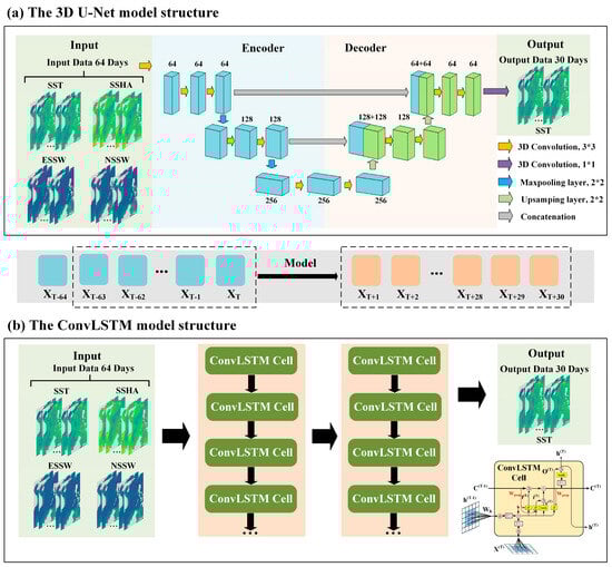
Figure 2. Flow chart for predicting SST in the SCS using the 3D U-Net model (a) and the ConvLSTM model (b), along with the forecasting strategies used by each model.

The encoder of the 3D U-Net model utilizes convolution and pooling operations in both spatial and temporal dimensions to capture variations in sea surface variables across different regions and times, enabling it to effectively learn relevant features. Subsequently, the decoder segment uses the features identified by the encoder to perform deconvolution and upsampling processes to map these features back to their original spatial and temporal scales, generating the prediction of future SST values, thereby accomplishing the task of forecasting SST in the SCS.

This is the first time the multivariable 3D U-Net model has been used for SST prediction in the SCS, representing a significant step forward in methodological approach. To thoroughly evaluate the performance of the 3D U-Net model, the ConvLSTM model, a widely recognized deep learning model shown in Figure 2b, was selected for comparison. The ConvLSTM model was proposed by Shi et al. [48] to address the shortcomings of the LSTM model in extracting two-dimensional spatial information. By adding convolution operations to the LSTM model, the ConvLSTM can learn and extract features in both temporal and spatial dimensions simultaneously. The model integrates current input and past states for predictions, governed by the input gate $i_t$, forget gate $f_t$, and output gate $o_t$. This controls the memory cell $C_t$and its final state $H_t$, enabling efficient spatiotemporal feature extraction. The primary equations of this process are as follows:

$$\begin{array}{l}{i}_t=\sigma \left(W_{xi}\ast X_t+W_{hi}\ast H_{t-1}+W_{ci}\circ C_{t-1}+b_i\right)\\ f_t=\sigma \left(W_{xf}\ast X_t+W_{hf}\ast H_{t-1}+W_{cf}\circ C_{t-1}+b_f\right)\\ C_t=f_t\circ C_{t-1}+i_t\circ \tan \mathrm{h}\left(W_{xc}\ast X_t+W_{hc}\ast H_{t-1}+b_c\right)\\ o_t=\sigma \left(W_{xo}\ast X_t+W_{ho}\ast H_{t-1}+W_{co}\circ C_t+b_o\right)\\ H_t=o_t\circ \tan \mathrm{h}\left(C_t\right)\end{array}$$

(3)

where $\sigma$ represents the sigmoid activation function, which can map values to a range between 0 and 1, $\ast$ denotes the convolutional operation introduced into the model, $\circ$ represents the Hadamard product, while tanh (·) denotes the hyperbolic tangent function. A comparison between our 3D U-Net model and the ConvLSTM model is particularly insightful. While the ConvLSTM model brings its strengths in handling spatiotemporal data, our 3D U-Net model introduces an innovative approach to multivariable integration for SST prediction. This comparative analysis aims to showcase the potential advantages and limitations of each model, providing a comprehensive understanding of their applicability in SST prediction within the unique context of the SCS.

Parameterization plays a key role in training deep learning models, often serving as a crucial determinant of their performance. Recognizing this, our study involves conducting extensive experiments to meticulously tune and optimize these parameters. This process, involving comparative analysis of various configurations, led us to identify the most effective parameter sets for our models. The details of these critical parameters, which significantly contributed to enhancing the models’ predictive accuracy, are comprehensively presented in Table 2.

Table 2. Parameters of the 3D U-Net and ConvLSTM models.

Models	Parameters
ConvLSTM	num_layers = 3, hidden_dim = [64, 64, 30], kernel_size = (3, 3), bias = True, return_all_layers = False, padding = 1	batch size: 12, activation function: elu, validation frequency: per epoch; loss function: mse, optimizer: radam, learning rate: 0.01, epoch: 1000, earlystopping;
3D U-Net	num_layers = 3, size = [64, 128, 256], groupnorm = 4, conv_kernel_size = 3, pool_kernel_size = 2, conv_padding = 1

To assess the performance of 3D U-Net for SST prediction, we selected four statistical indicators, including root mean square error (RMSE), Pearson correlation coefficient (R), mean absolute error (MAE) and mean absolute percentage error (MAPE). Each of these indicators offers a unique perspective on the model’s accuracy and reliability. The formulas for these statistical metrics are presented below, providing a mathematical basis for our evaluation methodology:

$$\begin{array}{l}\mathrm{RMSE}=\sqrt{\frac{{{\displaystyle \sum }}_{i=1}^n\left(y_i-{\widehat{y}}_i\right)}{n}}\\ \mathrm{R}=\frac{{{\displaystyle \sum }}_{i=1}^n\left(y_i-\overline{y}\right)\left({\widehat{y}}_i-\overline{\widehat{y}}\right)}{\sqrt{{{\displaystyle \sum }}_{i=1}^n{\left(y_i-\overline{y}\right)}^2}\sqrt{{{\displaystyle \sum }}_{i=1}^n{\left({\widehat{y}}_i-\overline{\widehat{y}}\right)}^2}}\\ \mathrm{MAE}=\frac{{{\displaystyle \sum }}_{i=1}^n\left|y_i-{\widehat{y}}_i\right|}{n}\\ \mathrm{MAPE}=\frac{100\%}{n}{\displaystyle \sum }_{i=1}^n\left|\frac{y_i-{\widehat{y}}_i}{y_i}\right|\end{array}$$

(4)

where $y_i$ is the observed SST, ${\widehat{y}}_i$ represents the SST predicted by the 3D U-Net model, and $\overline{y}$ and $\overline{\widehat{y}},$respectively, represent the mean of observed and predicted values.

3. Results

3.1. Comparison of the 3D U-Net Model with the ConvLSTM Model

To evaluate the 3D U-Net model’s performance in predicting SST in the SCS, we first compared it with the ConvLSTM model in terms of R and RMSE using data from 2021. Figure 3 shows the comparison of R and RMSE for SST predictions in the SCS using the 3D U-Net and ConvLSTM models for 1 to 30 day lead times throughout the year 2021.

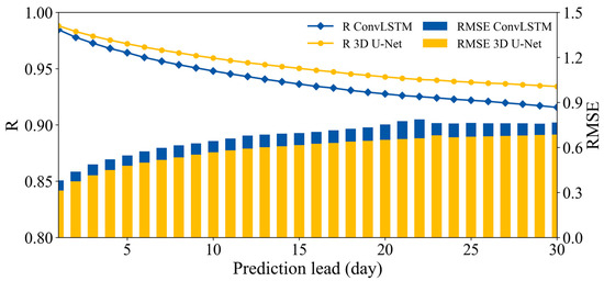
Figure 3. Performance comparison of the 3D U-Net and ConvLSTM models in predicting SST at different lead times in the SCS in 2021. Orange represents the 3D U-Net model, while blue represents the ConvLSTM model. The lines indicate R, and the bars indicate RMSE, calculated from all data used at different lead times in the test set.

Both the 3D U-Net and ConvLSTM models exhibited robust predictive performance over a 30-day forecast horizon in SST prediction, with high correlation (minimum value of R greater than 0.9) and low error (maximum value of RMSE less than 0.9 °C) (Figure 3). The results from both models, as the lead time increased from 1 to 30 days, consistently showed a decreasing trend in R and a corresponding increase in RMSE. This trend indicated a diminishing correlation between observed and predicted SST values and an incremental rise in forecast error as the prediction lead time lengthened. However, in a relative comparison across all prediction lead times, the 3D U-Net model consistently outperformed the ConvLSTM model, maintaining higher R values and lower RMSE. This outstanding performance of the 3D U-Net model, regarding forecast reliability, underscores its superior forecasting skill compared with the ConvLSTM model.

For a more detailed and objective evaluation of the two models, we also calculated various statistical indicators for SST predictions at different lead times, with the results presented in Table 3. At the 1-day lead time, the 3D U-Net model demonstrated superiority with an MAE of 0.23, compared with the ConvLSTM model’s MAE of 0.27. This trend of the 3D U-Net model outperforming the ConvLSTM model continued across RMSE and MAPE metrics. Although both models exhibited high R values, the 3D U-Net model (0.99) was slightly higher than the ConvLSTM model (0.98). Notably, as the forecast lead time extended to 7, 14, and 30 days, the model error increased, but the 3D U-Net model consistently maintained better performance across all metrics. Notably, on the 30th day, when the model performance dropped the most, the MAE, RMSE, MAPE, and R of the 3D U-Net model were 0.51, 0.69, 1.83%, and 0.93, respectively, which were still better than the ConvLSTM results of 0.57, 0.77, 2.01% and 0.92. Obviously, the 3D U-Net model achieved better forecasting performance at different lead times.

Table 3. Comparative statistical results of SST predictions by the ConvLSTM and 3D U-Net models at different lead times.

Models	Metrics	Prediction Lead (Day)
		1	7	14	30
ConvLSTM	MAE	0.27	0.43	0.51	0.57
	RMSE	0.38	0.60	0.69	0.77
	MAPE	0.95%	1.54%	1.81%	2.01%
	R	0.98	0.96	0.94	0.92
3D U-Net	MAE	0.23	0.39	0.46	0.51
	RMSE	0.31	0.52	0.61	0.69
	MAPE	0.83%	1.39%	1.64%	1.83%
	R	0.99	0.97	0.95	0.93

At the same time, we also compared the performance of the 3D U-Net and ConvLSTM models across different seasons, selecting February, May, August, and November to represent winter, spring, summer, and autumn, respectively. Forecasting errors (observed minus predicted values) were calculated for each season, and Gaussian kernel density estimation [49,50] was employed to analyze the distribution of these errors, as shown in Figure 4. The analysis revealed that the 3D U-Net model consistently achieved lower forecasting errors than the ConvLSTM model across all seasons, with errors being denser and closer to zero. Notably, while the kernel density curves for February and May (winter and spring) were somewhat sparser, indicating minor overestimation and underestimation, respectively, the 3D U-Net model’s curves remained comparatively denser and closer to zero. This pattern persisted even in the denser curves of August and November (summer and autumn). Overall, the 3D U-Net model demonstrated superior seasonal prediction performance compared with the ConvLSTM model.

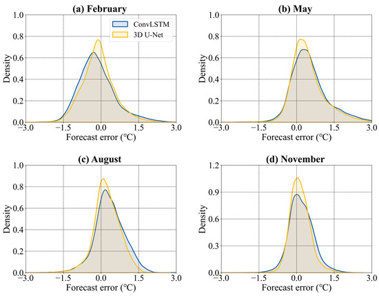
Figure 4. The Gaussian kernel density estimation of prediction errors (°C) for all lead times (1–30 days) in February, May, August, and November of 2021, using the 3D U-Net and ConvLSTM models.

3.2. Evaluation of the 3D U-Net Model

The above discussions show the 3D U-Net model’s better performance in SST prediction compared with the ConvLSTM model. This section delves further into evaluating the performance of the 3D U-Net model in the SCS from different perspectives. To thoroughly evaluate the accuracy of and correlation between the predictions of 3D U-Net and the observed values, we calculated the RMSE and R between the forecast results and observed values for each month in 2021 (the 30-day forecast results for each were based on data from the preceding 64 days). Throughout the year, the 3D U-Net model consistently showed lower RMSE (mainly within the range of 0–0.5 °C), and most R values exceeded 0.7, as depicted in Figure 5. Although error distribution varied monthly, larger errors predominantly occurred later in the forecast period, suggesting a gradual decline in model performance over time (Figure 5a). Figure 5b shows that, according to the distribution of R values, there was a positive correlation between the SST predicted by the 3D U-Net model and the observed values on most days in all months. However, from May to August, particularly in May, June, and August, the model experienced intermittent dips in correlation (R < 0.8). Notably, from September onwards, the correlation strength recovered significantly (R > 0.9), a pattern possibly linked to the SCS’s complex summer monsoon climate and circulation systems. Overall, the 3D U-Net model demonstrated relatively good performance across different months.

Figure 5. The distribution of (a) RMSE (°C) and (b) R values for all lead times (1–30 days) in SST prediction using the 3D U-Net model over 12 months in 2021.

Figure 6 presents the spatial distribution of RMSE and R between estimated and observed SST in the SCS for the year 2021. The generally low RMSE between SST predictions from the 3D U-Net model and observation in most areas of the SCS indicated a high degree of accuracy and correlation. Areas with relatively higher RMSE were identified primarily along the northern coast of the SCS, where the RMSE was in excess of 0.5 °C. In contrast, areas with relatively lower correlation coefficients, primarily situated in the southeastern parts of the SCS and showing R values below 0.9, are shown in Figure 6b. These findings further illustrate the 3D U-Net model’s reliability in accurately predicting SST in the SCS.

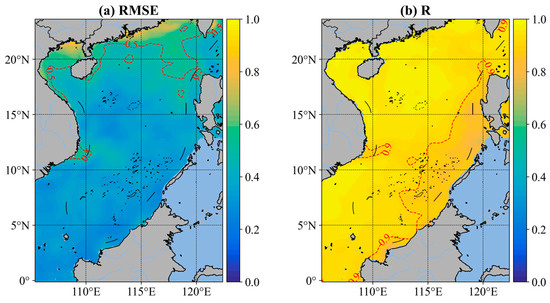
Figure 6. The spatial distribution of (a) RMSE (°C) and (b) R from the 2021 SST predictions in the SCS using the 3D U-Net model.

To thoroughly conduct a comprehensive assessment of the 3D U-Net model’s performance across different regions of the SCS, we selected four different areas, each with a range of 4° × 4°, labeled as boxes A, B, C, and D, as shown in Figure 7a. Box A (116.5° E–117.5° E, 19.5° N–20.5° N) encompassed an area near the southern continental shelf of China, while Box B (117.5° E–118.5° E, 16.5° N–17.5° N) aligned with the West Luzon eddy region. Box C (114.5° E–115.5° E, 11.5° N–12.5° N) encompassed an area near the central–southern SCS, with Box D (111° E–112° E, 15.5° N–16.5° N) near the eastern Vietnam eddy. The scatterplots in Figure 7b–e compare the SST predictions from the 3D U-Net model against observed SST across all data grids in the test set within these regions. The results indicated a robust positive linear correlation between predicted SST by the 3D U-Net model and observation in those typical areas, with most scatter points clustering near the line of equality, indicative of lower RMSE values and higher R values. The RMSE (R) values for these four regions were 0.54 °C (0.93), 0.48 °C (0.93), 0.36 °C (0.89), and 0.31 °C (0.96), respectively, underscoring the reliability and effectiveness of the 3D U-Net model in diverse areas of the SCS. In addition to RMSE and R, we further evaluated the performance of the 3D U-Net model at different lead times in the four regions using additional indicators, such as MAE and MAPE (Table 4). Through different indicators, the 3D U-Net demonstrated strong performance in all regions and lead times, marked by low error rates and strong correlations. Notably, while there was a slight decline in performance as lead times increased, the 3D U-Net model’s accuracy remained within a satisfactory range. This demonstrated the model’s robustness and reliability in diverse areas of the SCS.

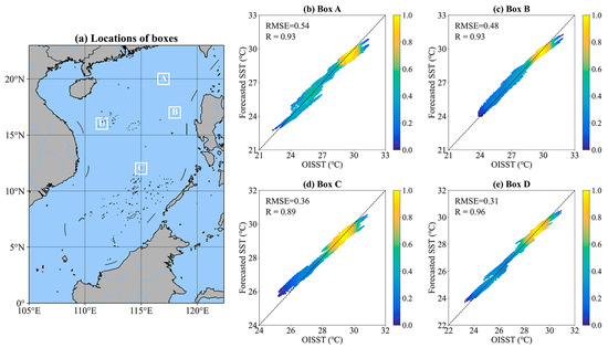
Figure 7. The four selected areas (Boxes A–D) used in this study, with Box A located at 116.5° E to 117.5° E, 19.5° N to 20.5° N; Box B at 117.5° E to 118.5° E, 16.5° N to 17.5° N; Box C at 114.5° E to 115.5° E, 11.5° N to 12.5° N; and Box D at 111° E to 112° E, 15.5° N to 16.5° N. Scatterplots compare SST predicted by the 3D U-Net model with observations across these regions (Boxes A–D) in 2021 (right panel).

Table 4. The statistical results of predictions from the 3D U-Net model at different lead times in four selected regions.

Area	Metrics	Prediction Lead (Day)
		1	7	14	30
Box A	MAE	0.25	0.51	0.61	0.72
	RMSE	0.33	0.65	0.78	0.91
	MAPE	0.91%	1.82%	2.20%	2.59%
	R	0.99	0.96	0.94	0.91
Box B	MAE	0.28	0.50	0.60	0.59
	RMSE	0.36	0.63	0.75	0.74
	MAPE	0.98%	1.75%	2.08%	2.06%
	R	0.99	0.95	0.93	0.93
Box C	MAE	0.19	0.36	0.44	0.47
	RMSE	0.25	0.46	0.54	0.60
	MAPE	0.67%	1.25%	1.55%	1.66%
	R	0.19	0.36	0.44	0.47
Box D	MAE	0.21	0.35	0.42	0.47
	RMSE	0.27	0.45	0.53	0.58
	MAPE	0.75%	1.26%	1.51%	1.69%
	R	0.99	0.97	0.95	0.94

Subsequently, we used the 3D U-Net model to predict SST in the SCS for 2021, with a cycle of 30 days. A time series analysis was performed for each of the four selected areas. Figure 8a–d illustrate the model’s SST time series predictions alongside observed data, representing the respective spatial average outcomes for Boxes A, B, C, and D. The comparison revealed that, aside from minor underestimations, the SST predicted by the 3D U-Net model was quite consistent with observed values. The RMSE (R) between the predicted and observed values was 0.44 (0.98), 0.42 (0.98), 0.29 (0.97), and 0.30 (0.99) for Boxes A, B, C, and D, respectively. These results highlight the 3D U-Net model’s robust and consistent predictive performance, even over extended lead times.

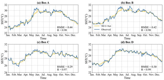
Figure 8. Spatially averaged time series comparison of SST for 2021, predicted by the 3D U-Net model and observed by satellites, including (a) Box A, (b) Box B, (c) Box C, and (d) Box D.

3.3. Comparison of Marine Heat Wave (MHW) Events

To further assess the capabilities of the 3D U-Net model, we evaluated its ability to forecast MHW events in the SCS for 2021 using the threshold method. We defined a relative threshold for MHW events as instances where the daily SST at a specific location surpassed the 90th percentile threshold, determined by seasonal variations across a climatological period of over 30 years. For this purpose, OISST data from 1982 to 2020 were utilized to compute the climatological baseline. An event was classified as an MHW if it persisted for at least five consecutive days, as per Hobday et al. [51]. Additionally, if the interval between consecutive events was less than two days, they were considered as a single event. The climate thresholds were calculated centered around an eleven-day window for each calendar day and smoothed out using a moving average method over thirty-one days. After identifying MHW events, four indicators were used to describe and compare MHW characteristics (as shown in Figure 9), including HWN, HWT, HWDU, and HWI, whose definitions can be found in Table 5 [52,53], where the cumulative intensity ${\displaystyle \sum }_j^{D_i}(T_{ij}-{\tilde{T}}_{ij})$ in a MHW event is the sum of the temperature anomaly intensity (temperature higher than the historical baseline) during the total duration (HWT) of each MHW, its unit is the “degree days”, and $T_{ij}$ and ${\tilde{T}}_{ij}$ are the values of SST and corresponding climatology during the MHW event.

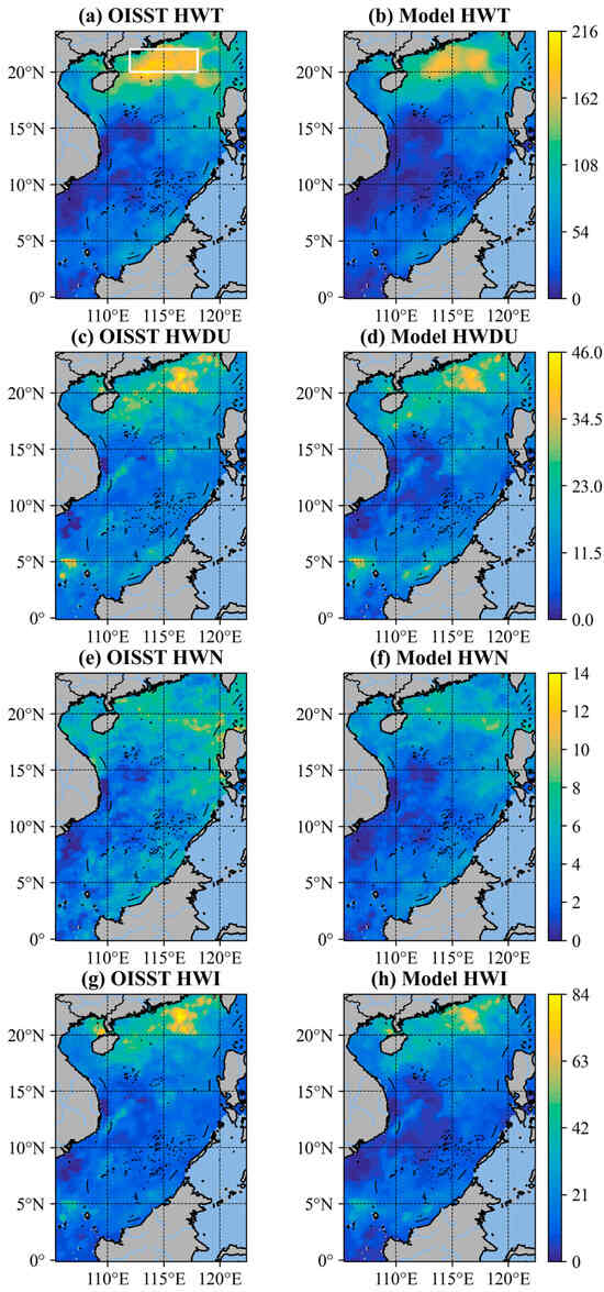
Figure 9. Spatial distribution of MHW characteristics in the SCS in 2021: (a,b) the total duration of MHW events (HWT), (c,d) the average duration of MHW events (HWDU), (e,f) the number of MHW events (HWN), and (g,h) the average cumulative intensity of MHW events (HWI). The observations are presented in the left panels, and the model predictions in the right panels. The white box in panel (a) indicates the representative area selected in this study.

Table 5. The definitions of the four MHW indices used in this study.

Index	Definition	Formulas	Unit
HWN	The number of MHW events	$HWN=N$	Times
HWT	The total duration of MHW events	$HWT={\displaystyle \sum }_{i=1}^N{D}_i$	Days
HWDU	The average duration of MHW events	$HWDU={\displaystyle \sum }_{i=1}^N\left(D_i\right)/N$	Days/time
HWI	The average cumulative intensity of MHW events	$HWI={\displaystyle \sum }_i^N{\displaystyle \sum }_j^{D_i}\left(T_{ij}-{\tilde{T}}_{ij}\right)/N$	Degree-days/time

As shown in Figure 9, the SST predicted by the 3D U-Net model and the observed SST showed good consistency in the numerical and spatial distribution of various statistical indicators of MHW events detected in the SCS. Prolonged MHW events were observed, particularly in the northern SCS (112° E–118° E, 20° N–22° N), with total durations exceeding 160 days (Figure 9a,b). Figure 9c,d show the average duration of these MHW events, which was similar to that of the total duration. In the areas with longer total duration, the average duration could reach 35 to 46 days. Conversely, the occurrence of MHW events was more dispersed across the area, with a notably higher frequency in the northern SCS compared with the south (Figure 9e,f). Figure 9g,h show that the spatial distributions of the average cumulative intensity of predicted and observed MHW events were relatively similar, and both showed apparent differences between south and north regions with high values mainly located in the northern part of the SCS, with the average cumulative intensity of each MHW event exceeding 45 degree-days. These comparisons demonstrate that the 3D U-Net model precisely forecasted and detected the various features of the MHW event that occurred in the SCS in 2021 and could help prevent disasters and climate changes caused by MHW events by predicting them in advance.

In 2021, the northern SCS experienced a high frequency and duration of MHW events, as shown in Figure 9. Consequently, we focused on a representative area (112° E–118° E, 20° N–22° N), marked by the white box in Figure 9a, to analyze the temporal dynamics of local MHW events (Figure 10). Since January 2021, this region has experienced multiple MHW events throughout all four seasons. Notably, two relatively intense and prolonged MHW events were observed from May to June and September to October. The 3D U-Net model successfully captured these occurrences, demonstrating its proficiency in predicting MHWs.

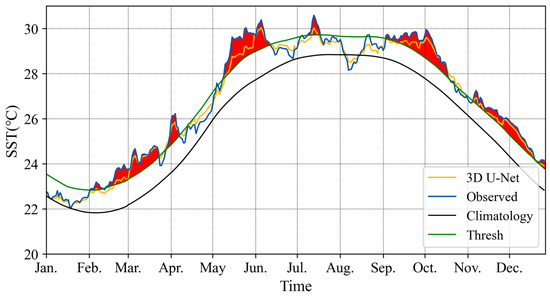
Figure 10. Seasonal variations of MHW events in the representative region in 2021. The curves depict the climatology (black), the 90th percentile seasonal threshold (green), the observed SST (blue), and the predicted SST (yellow), with the red area representing MHW events.

To more clearly demonstrate the performance of the 3D U-Net model during MHW events, we selected the longest-lasting MHW event in 2021 and provided a spatial distribution of some model prediction results during this period (Figure 11). Despite some minor discrepancies between the observed and predicted SST, the 3D U-Net model effectively captured SST distribution characteristics. Figure 12 presents the histograms of the SST difference during this period, offering a more detailed view of the discrepancy distribution. These histograms, primarily centered close to 0 °C, indicate that most prediction errors fell within the ±0.5 °C range. Collectively, Figure 11 and Figure 12 substantiate the 3D U-Net model’s robust predictive performance during MHW events in the SCS.

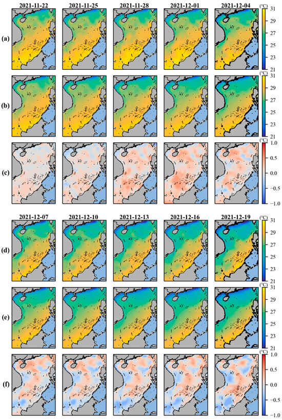
Figure 11. The SST prediction results by the 3D U-Net model (from 22 November 2021, to 21 December 2021, with a two-day interval displayed in the results) during MHW events in 2021. (a,d) show the observed SST. (b,e) show the predicted SST. (c,f) show the differences between observed and predicted values.

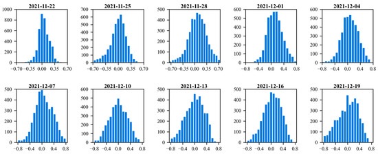
Figure 12. The deviation distribution in SST prediction results during MHW events from 22 November 2021, to 21 December 2021, displayed at two-day intervals.

To examine the relative contribution of different sea surface variables to SST prediction and MHW event detection in the SCS, a sensitivity experiment was performed using the 3D U-Net model. Figure 13 illustrates four different cases used in this sensitivity experiment. In the first group (Case 1), SSHA and SSW were introduced as input parameters based on SST. For the second group, SST and SSW were selected as predictors for SST (Case 2). In the third group (Case 3), SST and SSHA were used, while the fourth group (Case 4) relied solely on SST. The results revealed that the inclusion of SSHA and SSW alongside SST (Case 1) yielded the highest R values at various lead times, suggesting the best predictive performance (Figure 13). Conversely, the model relying solely on SST (Case 4) exhibited the lowest performance. This result indicated that SSHA and SSW are regulatory in SST forecasting and MHW event detection. The comparison of Case 2 with Case 3 revealed that SSW had a more significant impact on the model during the early stages of prediction, whereas the influence of SSHA became more pronounced as the lead time increased. These cases suggest that integrating SSHA and SSW could enhance the 3D U-Net model’s accuracy in the SCS.

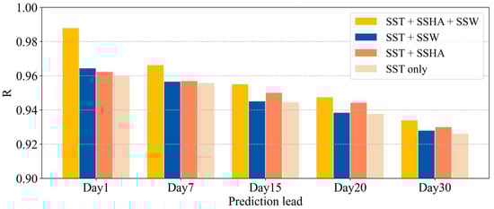
Figure 13. The comparison of R values at different lead times using various input variable combinations. Case 1 includes SST, SSHA, and SSW (yellow), Case 2 includes SST and SSW (blue), Case 3 includes SST and SSHA (orange), and Case 4 only relies on SST (beige).

4. Summary and Discussion

As an important parameter for oceanic and climatic systems, accurate prediction of SST is crucial. To achieve the prediction of SST using multi-source data, we developed a 3D U-Net model to predict SST in the SCS. Through comparative analysis with the ConvLSTM model across different lead times and seasons using various statistical indicators, the 3D U-Net model consistently demonstrated superior accuracy. RMSE values increased from 0.31 °C to 0.69 °C, while R values decreased from 0.99 to 0.93, outperforming ConvLSTM in all lead times ranging from 1 to 30 days. The Gaussian kernel density curves of prediction error for the 3D U-Net model in different seasons were more densely distributed near 0 than for the ConvLSTM model. Spatially, the 3D U-Net model predicted SST with lower error (RMSE < 0.5 °C) and higher correlation (R > 0.9) across most of the SCS. In different regions of the SCS, the scatterplots of predicted SST and observed SST showed that most scatter points clustered near the line of equality, indicative of lower RMSE values and higher R values. The RMSE (R) between the spatially averaged time series obtained from 3D U-Net predictions and observations were, respectively, 0.44 (0.98), 0.42 (0.98), 0.29 (0.97), and 0.30 (0.99) in the typical areas in 2021. These also suggest that 3D U-Net model predictions were consistent with the observed results in different areas of the SCS.

The 3D U-Net model’s proficiency was further evaluated by its performance during MHW events in 2021. The results detected by the 3D U-Net model predictions and those observed directly both noted the long-lasting MHW events occurring in the northern SCS in 2021. The total duration exceeded 160 days, with an average duration ranging from 35 to 46 days, and the average intensity of each MHW event exceeding 45 degree-days. Despite some differences, the 3D U-Net model demonstrated satisfactory prediction performance and ability to detect MHW events, which can be used to assist in taking proactive measures to protect marine ecosystems, prevent disasters, and better adapt to and mitigate the impacts of climate change. Finally, sensitivity experiments and statistical analyses highlighted the significant impact of different sea surface variables on SST prediction and MHW events detection. The results showed that SSHA and SSW have a significant effect on model prediction, which can improve accuracy and forecasting skills. Moreover, in the early stage of forecasting, SSW plays a crucial role in predicting SST, and as the lead time increases, the role of SSHA in predicting SST gradually increases, reflecting the complex interactions between variables.

In conclusion, the 3D U-Net model using multi-source sea surface variables proposed in this study performed well in predicting 30-day SST in the SCS, introducing an innovative approach for MHW event detection. The uniqueness of the 3D U-Net model is that its model structure is simple, but it can directly use multi-source sea surface variables to extract characteristic information of each variable, and more fully considers the interaction between variables. However, as a data-driven model, it faces limitations such as underestimation or overestimation, and the MHW is also affected by the influence of ocean dynamics and thermodynamics. Therefore, in future research, we plan to integrate more ocean dynamic mechanisms into the model to improve SST and MHW prediction accuracy and forecasting skills. Furthermore, this model can be applied to forecasting additional essential ocean parameters such as SSW, sea surface height, and thermohaline structure, providing new ideas for future research work, so that it can play a more comprehensive role in marine disaster prevention, marine ranching, and environmental protection.

References

- McPhaden, M.J.; Busalacchi, A.J.; Cheney, R.; Donguy, J.R.; Gage, K.S.; Halpern, D.; Ji, M.; Julian, P.; Meyers, G.; Mitchum, G.T. The Tropical Ocean-Global Atmosphere observing system: A decade of progress. J. Geophys. Res. Ocean. 1998, 103, 14169–14240. [Google Scholar] [CrossRef]
- Namias, J.; Cayan, D.R. Large-scale air-sea interactions and short-period climatic fluctuations. Science 1981, 214, 869–876. [Google Scholar] [CrossRef]
- Neelin, J.; Latif, M.; Allaart, M.; Cane, M.; Cubasch, U.; Gates, W.; Gent, P.; Ghil, M.; Gordon, C.; Lau, N. Tropical air-sea interaction in general circulation models. Clim. Dyn. 1992, 7, 73–104. [Google Scholar] [CrossRef]
- Alexander, L.V.; Uotila, P.; Nicholls, N. Influence of sea surface temperature variability on global temperature and precipitation extremes. J. Geophys. Res. Atmos. 2009, 114, D18. [Google Scholar] [CrossRef]
- McGowan, J.A.; Cayan, D.R.; Dorman, L.M. Climate-ocean variability and ecosystem response in the Northeast Pacific. Science 1998, 281, 210–217. [Google Scholar] [CrossRef]
- Wang, C.; Fiedler, P.C. ENSO variability and the eastern tropical Pacific: A review. Prog. Oceanogr. 2006, 69, 239–266. [Google Scholar] [CrossRef]
- Behera, S.K.; Yamagata, T. Subtropical SST dipole events in the southern Indian Ocean. Geophys. Res. Lett. 2001, 28, 327–330. [Google Scholar] [CrossRef]
- Feng, M.; Meyers, G. Interannual variability in the tropical Indian Ocean: A two-year time-scale of Indian Ocean Dipole. Deep Sea Res. Part II Top. Stud. Oceanogr. 2003, 50, 2263–2284. [Google Scholar] [CrossRef]
- Yu, K. Coral reefs in the South China Sea: Their response to and records on past environmental changes. Sci. China Earth Sci. 2012, 55, 1217–1229. [Google Scholar] [CrossRef]
- Chang, S.W.; Madala, R.V. Numerical simulation of the influence of sea surface temperature on translating tropical cyclones. J. Atmos. Sci. 1980, 37, 2617–2630. [Google Scholar] [CrossRef][Green Version]
- Vecchi, G.A.; Soden, B.J. Effect of remote sea surface temperature change on tropical cyclone potential intensity. Nature 2007, 450, 1066–1070. [Google Scholar] [CrossRef]
- Yu, J.; Li, T.; Tan, Z.; Zhu, Z. Effects of tropical North Atlantic SST on tropical cyclone genesis in the western North Pacific. Clim. Dyn. 2016, 46, 865–877. [Google Scholar] [CrossRef]
- Qiao, F.; Yuan, Y.; Yang, Y.; Zheng, Q.; Xia, C.; Ma, J. Wave-induced mixing in the upper ocean: Distribution and application to a global ocean circulation model. Geophys. Res. Lett. 2004, 31, 11. [Google Scholar] [CrossRef]
- Yang, Q.; Zhao, W.; Liang, X.; Tian, J. Three-dimensional distribution of turbulent mixing in the South China Sea. J. Phys. Oceanogr. 2016, 46, 769–788. [Google Scholar] [CrossRef]
- Roxy, M.; Tanimoto, Y. Influence of sea surface temperature on the intraseasonal variability of the South China Sea summer monsoon. Clim. Dyn. 2012, 39, 1209–1218. [Google Scholar] [CrossRef]
- Liu, Q.; Jiang, X.; Xie, S.P.; Liu, W.T. A gap in the Indo-Pacific warm pool over the South China Sea in boreal winter: Seasonal development and interannual variability. J. Geophys. Res. Ocean. 2004, 109, C7. [Google Scholar] [CrossRef]
- Su, J. Overview of the South China Sea circulation and its influence on the coastal physical oceanography outside the Pearl River Estuary. Cont. Shelf Res. 2004, 24, 1745–1760. [Google Scholar] [CrossRef]
- Liu, Q.; Kaneko, A.; Su, J. Recent progress in studies of the South China Sea circulation. J. Oceanogr. 2008, 64, 753–762. [Google Scholar] [CrossRef]
- Vaid, B.; Preethi, B.; Kripalani, R. The Asymmetric Influence of the South China Sea Biweekly SST on the abnormal Indian monsoon rainfall of 2002. Pure Appl. Geophys. 2018, 175, 4625–4642. [Google Scholar] [CrossRef]
- Krishnamurti, T.; Chakraborty, A.; Krishnamurti, R.; Dewar, W.K.; Clayson, C.A. Seasonal prediction of sea surface temperature anomalies using a suite of 13 coupled atmosphere–ocean models. J. Clim. 2006, 19, 6069–6088. [Google Scholar] [CrossRef]
- Li, W.; Xie, Y.; He, Z.; Han, G.; Liu, K.; Ma, J.; Li, D. Application of the multigrid data assimilation scheme to the China Seas’ temperature forecast. J. Atmos. Ocean. Technol. 2008, 25, 2106–2116. [Google Scholar] [CrossRef]
- Stockdale, T.N.; Balmaseda, M.A.; Vidard, A. Tropical Atlantic SST prediction with coupled ocean–atmosphere GCMs. J. Clim. 2006, 19, 6047–6061. [Google Scholar] [CrossRef]
- Johnson, S.D.; Battisti, D.S.; Sarachik, E. Empirically derived Markov models and prediction of tropical Pacific sea surface temperature anomalies. J. Clim. 2000, 13, 3–17. [Google Scholar] [CrossRef]
- Xue, Y.; Leetmaa, A. Forecasts of tropical Pacific SST and sea level using a Markov model. Geophys. Res. Lett. 2000, 27, 2701–2704. [Google Scholar] [CrossRef]
- Landman, W.A.; Mason, S.J. Forecasts of near-global sea surface temperatures using canonical correlation analysis. J. Clim. 2001, 14, 3819–3833. [Google Scholar] [CrossRef]
- Kug, J.S.; Kang, I.S.; Lee, J.Y.; Jhun, J.G. A statistical approach to Indian Ocean sea surface temperature prediction using a dynamical ENSO prediction. Geophys. Res. Lett. 2004, 31, 9. [Google Scholar] [CrossRef]
- Lins, I.D.; Araujo, M.; das Chagas Moura, M.; Silva, M.A.; Droguett, E.L. Prediction of sea surface temperature in the tropical Atlantic by support vector machines. Comput. Stat. Data Anal. 2013, 61, 187–198. [Google Scholar] [CrossRef]
- Aparna, S.; D’souza, S.; Arjun, N. Prediction of daily sea surface temperature using artificial neural networks. Int. J. Remote Sens. 2018, 39, 4214–4231. [Google Scholar] [CrossRef]
- Patil, K.; Deo, M.C. Prediction of daily sea surface temperature using efficient neural networks. Ocean Dyn. 2017, 67, 357–368. [Google Scholar] [CrossRef]
- Liu, J.; Tang, Y.; Wu, Y.; Li, T.; Wang, Q.; Chen, D. Forecasting the Indian Ocean Dipole with deep learning techniques. Geophys. Res. Lett. 2021, 48, e2021GL094407. [Google Scholar] [CrossRef]
- Zhang, Q.; Wang, H.; Dong, J.; Zhong, G.; Sun, X. Prediction of sea surface temperature using long short-term memory. IEEE Geosci. Remote Sens. Lett. 2017, 14, 1745–1749. [Google Scholar] [CrossRef]
- Choi, H.-M.; Kim, M.-K.; Yang, H. Deep-learning model for sea surface temperature prediction near the Korean Peninsula. Deep Sea Res. Part II Top. Stud. Oceanogr. 2023, 208, 105262. [Google Scholar] [CrossRef]
- Xiao, C.; Chen, N.; Hu, C.; Wang, K.; Gong, J.; Chen, Z. Short and mid-term sea surface temperature prediction using time-series satellite data and LSTM-AdaBoost combination approach. Remote Sens. Environ. 2019, 233, 111358. [Google Scholar] [CrossRef]
- Yang, Y.; Dong, J.; Sun, X.; Lima, E.; Mu, Q.; Wang, X. A CFCC-LSTM model for sea surface temperature prediction. IEEE Geosci. Remote Sens. Lett. 2017, 15, 207–211. [Google Scholar] [CrossRef]
- Taylor, J.; Feng, M. A deep learning model for forecasting global monthly mean sea surface temperature anomalies. Front. Clim. 2022, 4, 178. [Google Scholar] [CrossRef]
- Song, T.; Jiang, J.; Li, W.; Xu, D. A deep learning method with merged LSTM neural networks for SSHA prediction. IEEE J. Sel. Top. Appl. Earth Obs. Remote Sens. 2020, 13, 2853–2860. [Google Scholar] [CrossRef]
- Hao, P.; Li, S.; Song, J.; Gao, Y. Prediction of Sea Surface Temperature in the South China Sea Based on Deep Learning. Remote Sens. 2023, 15, 1656. [Google Scholar] [CrossRef]
- Shao, Q.; Li, W.; Han, G.; Hou, G.; Liu, S.; Gong, Y.; Qu, P. A deep learning model for forecasting sea surface height anomalies and temperatures in the South China Sea. J. Geophys. Res. Ocean. 2021, 126, e2021JC017515. [Google Scholar] [CrossRef]
- Miao, Y.; Zhang, C.; Zhang, X.; Zhang, L. A Multivariable Convolutional Neural Network for Forecasting Synoptic-Scale Sea Surface Temperature Anomalies in the South China Sea. Weather Forecast. 2023, 38, 849–863. [Google Scholar] [CrossRef]
- Huang, B.; Liu, C.; Banzon, V.; Freeman, E.; Graham, G.; Hankins, B.; Smith, T.; Zhang, H.-M. Improvements of the daily optimum interpolation sea surface temperature (DOISST) version 2.1. J. Clim. 2021, 34, 2923–2939. [Google Scholar] [CrossRef]
- Atlas, R.; Hoffman, R.N.; Ardizzone, J.; Leidner, S.M.; Jusem, J.C.; Smith, D.K.; Gombos, D. A cross-calibrated, multiplatform ocean surface wind velocity product for meteorological and oceanographic applications. Bull. Am. Meteorol. Soc. 2011, 92, 157–174. [Google Scholar] [CrossRef]
- Fernández, J.G.; Abdellaoui, I.A.; Mehrkanoon, S. Deep coastal sea elements forecasting using UNet-based models. Knowl.-Based Syst. 2022, 252, 109445. [Google Scholar] [CrossRef]
- Ren, Y.; Li, X. Predicting the Daily Sea Ice Concentration on a Sub-Seasonal Scale of the Pan-Arctic During the Melting Season by a Deep Learning Model. IEEE Trans. Geosci. Remote Sens. 2023, 61, 4301315. [Google Scholar] [CrossRef]
- Wang, Y.; Yuan, X.; Ren, Y.; Bushuk, M.; Shu, Q.; Li, C.; Li, X. Subseasonal prediction of regional Antarctic sea ice by a deep learning model. Geophys. Res. Lett. 2023, 50, e2023GL104347. [Google Scholar] [CrossRef]
- Ronneberger, O.; Fischer, P.; Brox, T. U-net: Convolutional networks for biomedical image segmentation. In Proceedings of the Medical Image Computing and Computer-Assisted Intervention 2015, Munich, Germany, 5–9 October 2015; pp. 234–241. [Google Scholar] [CrossRef]
- Çiçek, Ö.; Abdulkadir, A.; Lienkamp, S.S.; Brox, T.; Ronneberger, O. 3D U-Net: Learning dense volumetric segmentation from sparse annotation. In Proceedings of the International Conference on Medical Image Computing and Computer-Assisted Intervention, Athens, Greece, 17–21 October 2016; Springer: Cham, Switzerland, 2016; pp. 424–432. [Google Scholar] [CrossRef]
- Ji, S.; Xu, W.; Yang, M.; Yu, K. 3D convolutional neural networks for human action recognition. IEEE Trans. Pattern Anal. Mach. Intell. 2012, 35, 221–231. [Google Scholar] [CrossRef]
- Shi, X.; Chen, Z.; Wang, H.; Yeung, D.-Y.; Wong, W.-K.; Woo, W.-c. Convolutional LSTM network: A machine learning approach for precipitation nowcasting. Adv. Neural Inf. Process. Syst. 2015, 28, 1. [Google Scholar]
- Terrell, G.R.; Scott, D.W. Variable kernel density estimation. Ann. Stat. 1992, 20, 1236–1265. [Google Scholar] [CrossRef]
- Silverman, B.W. Density Estimation for Statistics and Data Analysis; Routledge: London, UK, 2018. [Google Scholar] [CrossRef]
- Hobday, A.J.; Alexander, L.V.; Perkins, S.E.; Smale, D.A.; Straub, S.C.; Oliver, E.C.; Benthuysen, J.A.; Burrows, M.T.; Donat, M.G.; Feng, M. A hierarchical approach to defining marine heatwaves. Prog. Oceanogr. 2016, 141, 227–238. [Google Scholar] [CrossRef]
- Wang, P.; Tang, J.; Sun, X.; Wang, S.; Wu, J.; Dong, X.; Fang, J. Heat waves in China: Definitions, leading patterns, and connections to large-scale atmospheric circulation and SSTs. J. Geophys. Res. Atmos. 2017, 122, 10679–10699. [Google Scholar] [CrossRef]
- Yao, Y.; Wang, C. Variations in summer marine heatwaves in the South China Sea. J. Geophys. Res. Ocean. 2021, 126, e2021JC017792. [Google Scholar] [CrossRef]
Disclaimer/Publisher’s Note: The statements, opinions and data contained in all publications are solely those of the individual author(s) and contributor(s) and not of MDPI and/or the editor(s). MDPI and/or the editor(s) disclaim responsibility for any injury to people or property resulting from any ideas, methods, instructions or products referred to in the content. |
© 2024 by the authors. Licensee MDPI, Basel, Switzerland. This article is an open access article distributed under the terms and conditions of the Creative Commons Attribution (CC BY) license (https://creativecommons.org/licenses/by/4.0/).