Climate Driver Influences on Prediction of the Australian Fire Behaviour Index

Abstract

Fire danger poses a pressing threat to ecosystems and societies worldwide. Adequate preparation and forewarning can help reduce these threats, but these rely on accurate prediction of extreme fire danger. With the knowledge that climatic conditions contribute heavily to overall fire danger, this study evaluates the skill with which episodes of extreme fire danger in Australia can be predicted from the activity of large-scale climate driver patterns. An extremal dependence index for extreme events is used to depict the historical predictive skill of the Australian Bureau of Meteorology’s subseasonal climate prediction system in replicating known relationships between the probability of top-decile fire danger and climate driver states at a lead time of 2–3 weeks. Results demonstrate that the El Niño Southern Oscillation, Southern Annular Mode, persistent modes of atmospheric blocking, Indian Ocean Dipole and Madden-Julian Oscillation are all key for contributing to predictability of fire danger forecasts in different regions during critical fire danger periods. Northwest Australia is found to be particularly predictable, with the highest mean index differences (>0.50) when certain climate drivers are active, compared with the climatological index mean. This integrated approach offers a valuable resource for decision-making in fire-prone regions, providing greater confidence to users relying on fire danger outlooks for key management decisions, such as those involved in the sectors of national park and forest estate management, agriculture, emergency services, health and energy. Furthermore, the results highlight strengths and weaknesses in both the Australian Fire Danger Rating System and the operational climate model, contributing additional information for improving and refining future iterations of these systems.

1. Introduction

Australia is heavily affected by bushfires, which, despite their importance to the Australian landscape, have undergone considerable regime shifts in recent decades [1,2], becoming difficult for humans to manage and ecosystems to tolerate. Observed extreme fire events are exemplified by landmark seasons such as the 2003 southeast Australian fires [3], the Black Saturday fires of 2009 [4] and, more recently, the Black Summer season of 2019/2020 [5]. Each of these events had abnormally severe impacts. Cases of fires with unusually large burned areas, fatalities, house and property loss and ecological ramifications are those which should guide and advise future fire management and preparation activities [6,7,8]. Following the 2019/2020 fires, the world experienced a multiyear “triple-dip” La Niña event [9] which allowed high fuel loads to accumulate [10,11], fuelling dangerous grass fires in inland New South Wales (NSW) in February 2023, and increasing the potential for another catastrophic bushfire season [10,11]. Conditions were expected to turn drier over the Austral spring and summer [12], decreasing fuel moisture and priming these fuels to burn. This pattern of floods and fires is not limited to this example. Such a cycle has been observed throughout Australia’s history [10,11,13,14]. However, with a developing field of research on the potential changes in El Niño–Southern Oscillation behaviour and the effects of a warming climate on fire conditions, protecting Australia’s natural, built and human assets is of utmost importance.

Landowners and property managers are a group of stakeholders with a high level of involvement, engagement and interest in this area of asset protection against fire threat [15], especially in agricultural or pastural regions of Australia where land management is a primary factor in securing their livelihoods. Many decisions regarding their practices and activities are dependent on the fire outlook [15]. A high confidence in the seasonal outlooks is therefore an important aspect of their decision-making. It also supports fire management agencies in their preparation and suppression activities and encourages concerted action and awareness in a range of other sectors of society.

In this study, we assess the capability of the Australian Bureau of Meteorology’s subseasonal to seasonal climate prediction system to predict the occurrence of extreme fire danger associated with dominant climate drivers which impact Australia [16]. This assessment demonstrates the climate drivers that have historically led to higher or lower accuracy in fire danger forecasts than is normal across the entire hindcast period. This can provide important information regarding the expected accuracy of current and future fire behaviour outlooks and highlight potential areas for improvement of forecast accuracy, informed by the climate drivers active at any given time.

2. Materials and Methods

Australian fire danger is currently operationally monitored and expressed using the Australian Fire Danger Rating System (AFDRS). This system has recently replaced the McArthur [17] fire danger rating system based on forest and grass indices. The Fire Behaviour Index (FBI) metric of the AFDRS is used to express overall fire danger. This numerical scale varies from 0 to 100+ and is normalised across all fuel types and environments of Australia. It was developed based on the characteristics of fire behaviour which were determined to be the key indicators of fire danger in each fuel type. In most fuel types, potential fireline intensity was used, but some fuels such as spinifex and buttongrass utilise other metrics of fire behaviour (e.g., rate of spread [18]). Overall, the aim of the FBI metric is to indicate the potential hazard from various aspects related to fire behaviour such as rate of spread, difficulty of suppression or risk to life and property. Although the Fire Behaviour Index (FBI) utilises a standardised 1–100+ scale, the underlying thresholds for fire behaviour metrics, such as fire intensity, exhibit inherent variability across different fuel types. This scaling approach, while advantageous for simplicity and comparison, unavoidably masks some nuanced details specific to each fuel type. Furthermore, the calculation of the FBI for each fuel type necessitates incorporating multiple input parameters, exceeding the scope of this report for exhaustive enumeration. However, we offer insights into several key datasets employed in this study:

• Grassland fuel loads: Characterised based on Köppen climate zones, these were assumed to be constant throughout the climatology.
• Time-since-fire: Employed for all fuel types except pine, grassland, and grassy woodland, these data extend back to 2003 (Gregory, P., personal communication).
• Generic fuel state: Inputs relied on established models from relevant literature with tailored adjustments and assumptions in some instances.
• Jurisdictional fuel datasets: These, along with associated research documents, informed decisions regarding overstorey subtypes and coverage values (Matthews, 2023, personal communication).

Readers seeking comprehensive details on the FBI calculations for each fuel type and the underlying models are directed to the AFDRS technical guides [18], the AFDRS Research Prototype report [19], and the Bureau of Meteorology Fire Behaviour Model Guides [20].

The AFDRS is a modular system designed to be updateable to incorporate the latest developments and understanding of fire science. As a result, there is an added level of uncertainty in AFDRS products, as the underlying models and science are likely to be changeable for some time as shortcomings of the recently implemented system are identified and improved upon. Therefore, although the most recent data have been used in this study, further changes after publication may produce varying results. In addition, the system has known limitations. For many fuel types, an adequate fuel state history has been unavailable, so existing fuel availability models were adapted to attempt to account for missing data, and these adaptations did not always have an adequate scientific foundation [18]. The hindcast period of 2003–2017 is a further limitation. This available hindcast limits the climatology to a warmer and wetter period than an average climate state extending further back in time [21], limits the use of the system in environments with longer fire intervals and precludes analysis of longer-term patterns and variations associated with such phenomena as the Pacific Decadal Oscillation or Interdecadal Pacific Oscillation.

We aim to demonstrate the potential for known relationships between FBI and six drivers of Australian climate variability to add to the skill with which a subseasonal-to-seasonal climate simulation model forecasts episodes of top-decile FBI. The Australian Community Climate and Earth System Simulator-Seasonal forecast system version 2 (ACCESS-S2) is the current operational forecasting system used by the Australian Bureau of Meteorology. ACCESS-S2 is based on the UK Met Office’s GloSea5 global model and has an atmospheric horizontal resolution of ~60 km and 84 vertical levels. The primary updates from its predecessor, ACCESS-S1, are in initialisation and postprocessing. Initialisation of soil moisture, ocean and sea ice fields is now generated using weakly coupled data assimilation, whereas climatology was used previously. Full details of ACCESS-S2 are documented by Wedd et al. [22]. This study uses the hindcast FBI data from ACCESS-S2, which comprise a 279-day integration initialised on the 1st, 6th, 11th, 16th, 21st and 26th of each month using three ensemble members. We use FBI 7-day running mean hindcasts at 7–14 days and 15–21 days verification dates. These are matched to observed FBI 7-day means at the verification dates, and aggregated into Austral seasons (DJF, MAM, JJA and SON) also based on the verification, not the initiation date.

The choice of climate drivers (

Table 1. Indices defining climate drivers in an evaluation of their impacts on Australian fire danger.

Driver	Index	Reference Study
Madden-Julian Oscillation (MJO)	Real-time Multivariate MJO series 1 and 2	Wheeler & Hendon, 2004 [34]
El Niño Southern Oscillation (ENSO)	NINO-3.4	Trenberth, 1997 [35]
Indian Ocean Dipole (IOD)	Dipole Mode Index	Saji & Yamagata, 2003 [36]
Southern Annular Mode (SAM)	Antarctic Oscillation Index	Gong & Wang, 1999 [37]
Split-Flow Blocking	Blocking Index	Pook & Gibson, 1999 [38]
Subtropical Ridge Highs (STRH)	STRH Index	Marshall et al., 2014 [23]

) is based upon the results of previous analyses showing their significant influences on Australian climate (e.g., [23,24,25,26,27]) and fire danger [16,28]. These are the El Niño Southern Oscillation (ENSO), Indian Ocean Dipole (IOD), Southern Annular Mode (SAM), Madden-Julian Oscillation (MJO), split-flow blocking and persistent modes of high pressure in the region of the Tasman Sea (STRH). Following the methods used by Marshall et al. [16] and Taylor et al. [28], we use meteorological data from NCEP/NCAR Reanalysis 1 [29] to compute climate driver indices and define the high and low polarities when the driver is >1 SD above or below its 2003–2017 mean. For the observed and ACCESS-S2 simulated FBI, we stratify the dates in the datasets according to when the climate driver under investigation is in the phase of interest. For each date the given climate driver phase was active, we build the probability that the FBI at a grid location is above the 90th percentile. This overall probability is then divided by the climatological rate of occurrence (which is 0.1), to produce a probability ratio. This is a way of expressing the change in likelihood of extreme FBI that occurs coincident with the climate driver phase of interest. For example, a probability ratio of 2 equates to a doubling in the chance of extreme FBI, or a 100% increase in the likelihood. We then assess how reliably ACCESS-S2 can (a) forecast the observed chance of extreme fire danger under all conditions and (b) add skill to these forecasts when each mode of a climate driver is active. This assessment is performed using the Symmetric Extremal Dependence Index (SEDI) [30]. The SEDI was designed for the verification of rare binary events. Verification of rare event forecasts is difficult because, as rarity increases, a forecast that (for example) predicts only non-events can yield high accuracy scores using most verification methods when it is, in fact, meaningless. The SEDI overcomes this obstacle and those of a number of extreme dependency scores by being nondegenerate and also independent of the base rate. It has been shown to perform well for 90th percentile events across several climatological variables [16,30,31,32]. It is based on a 2 × 2 contingency table of observed and predicted forecasts, where a “hit” is scored when both the forecast and the observations exceed the 90th percentile of FBI, and a “false alarm” is scored when extreme FBI is forecast but not observed. SEDI can be thought of as similar to the Odds Ratio Skill Score, in that it is a transformation of the Odds Log Ratio. In this sense, it incorporates many of the strengths of the Odds Ratio and Odds Ratio Skill Score. Unlike the Odds Ratio Skill Score, SEDI does not degenerate to −1 or 1 for rare events [30]. It is the Australian Bureau of Meteorology’s and the Commonwealth Scientific and Industrial Research Organisation’s recommended approach for forecasting rare and extreme events [33]. To align with the use of the Australian Bureau of Meteorology’s forecast system and the Australian focus of this study, SEDI was considered the most appropriate verification metric for this study, and also found to be one of the most accurate and useful verification metrics for rare 90th percentile event forecasting. The SEDI at each grid location is then scored using Equation (1):

$$SEDI=\frac{logF-logH-log(1-F)+log(1-H)}{logF+logH+log(1-F)+log(1-H)}$$

(1)

where H = hit rate and F = false alarm rate. Scores range from −1 to 1, where negative scores represent worse skill than a random forecast, and positive scores represent better skill, with 1 being a perfect forecast. Following [16], forecasts from each of the three ensemble members are added separately to the total scores in the contingency table. The confidence interval of the SEDI score is estimated using standard error (S_SEDI):

$${\mathrm{S}}_{\mathrm{SEDI}}=\frac{2|\frac{\left(1-H\right)\left(1-F\right)+HF}{(1-H(1-F\left)\right)}\log \left[F\left(1-H\right)\right]+\frac{2H}{1-H}\mathrm{l}\mathrm{o}\mathrm{g}[H\left(1-F\right)]|}{{H\{\log \left[F\left(1-H\right)\right]+\log \left[H\left(1-F\right)\right]\}}^2}\sqrt{\frac{\left(H\right(1-H)}{pn}}$$

(2)

where pn = a + c, the total observed events, as defined by Ferro and Stephenson [30] in their Table 1. We use 1.645 S_SEDI to estimate the 90% confidence interval at each grid point, assuming that S_SEDI approximates the standard deviation. A SEDI score is taken as significant when SEDI—1.645 S_SEDI > 0.

3. Results and Discussion

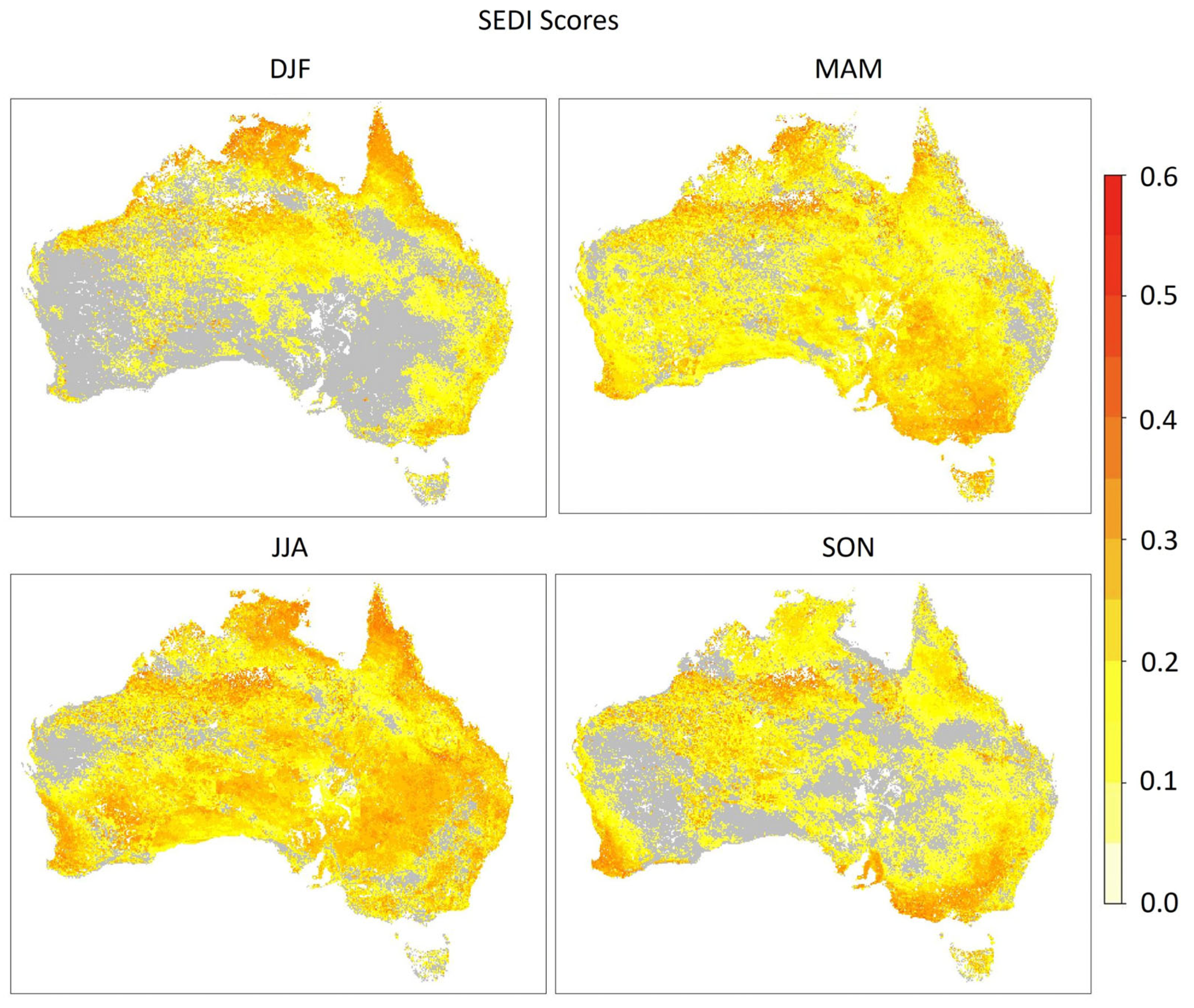
3.1. Prediction of Extreme Fire Behaviour Index

We begin by computing the forecast skill of ACCESS-S2 to predict extreme FBI using all available forecasts for each season (Figure 1). These skill maps represent the general forecast skill, and the SEDI scores stratified by driver and phase are subtracted from these base maps to show where the stratification results in a more or less skilful forecast of extreme FBI.

The overall predictions of extreme FBI in ACCESS-S2 are skilful across most of the continent in MAM, JJA and SON. Areas of significant positive SEDI scores are restricted in DJF to the north and east of Australia and the northern desert regions. They maximise in the far north, in Arnhem Land at the Cape York Peninsula. This is problematic, given that DJF is the active fire season in most of Southern Australia. Predictive skill is still available in areas of southeast Australia, which may allow for some assumptions to be drawn about the surrounding areas in Victoria and NSW.

In MAM, the predictive skill is more encouraging, with positive scores over almost the entire continent, maximising in Victoria, inland NSW, southwest Western Australia and parts of Arnhem Land and the Cape York Peninsula. The maximisation of skill in southern regions is consistent with understanding that high fire danger in MAM has historically been most common in the southern extremities of the continent [2,39], while noting that there is a trend towards increasing hazardous fire weather and an expansion of areas prone to high fire danger in autumn [1,2,40].

JJA shows similar patterns of significant predictive skill to MAM. High skill is available in the north of Australia, most of NSW and a larger area of southwest Western Australia. This is encouraging for potential forecasting applications in the tropical fire season and central desert regions, which may experience an increase in fire danger during JJA [40].

A decrease in the areas with significant forecasting capacity occurs in SON, which is again problematic, given not only the large portion of Australia prone to high fire danger in this season [2,39,40] but also the considerable trend towards increasing fire danger in SON [41,42,43,44,45]. SEDI scores are highest during this season in southeast and southwest Australia, which are areas prone to high fire danger in spring [39,40], but increases in severe fire conditions are projected for central and northwest Australia [40], which have incomplete predictive skill in ACCESS-S2.

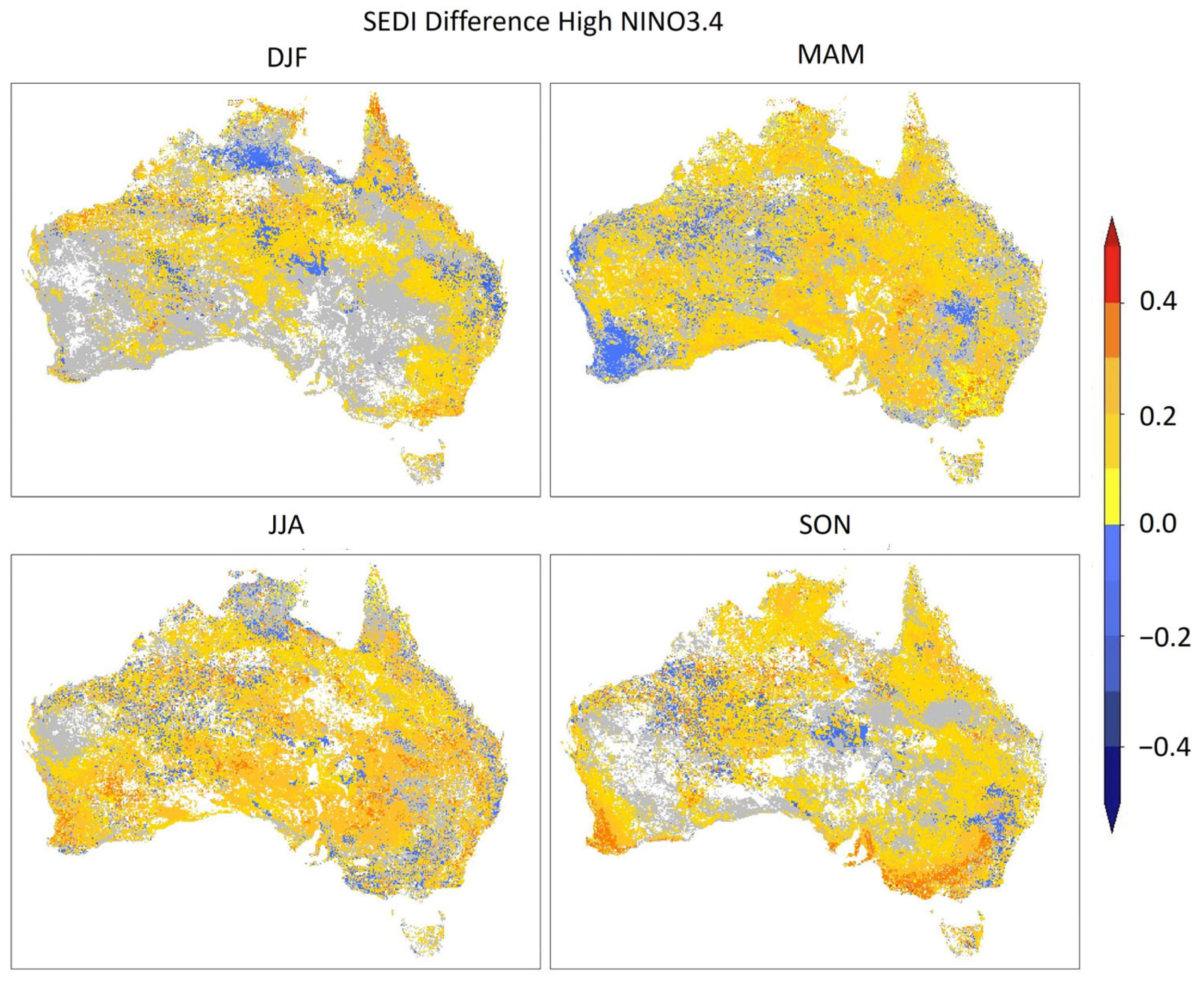
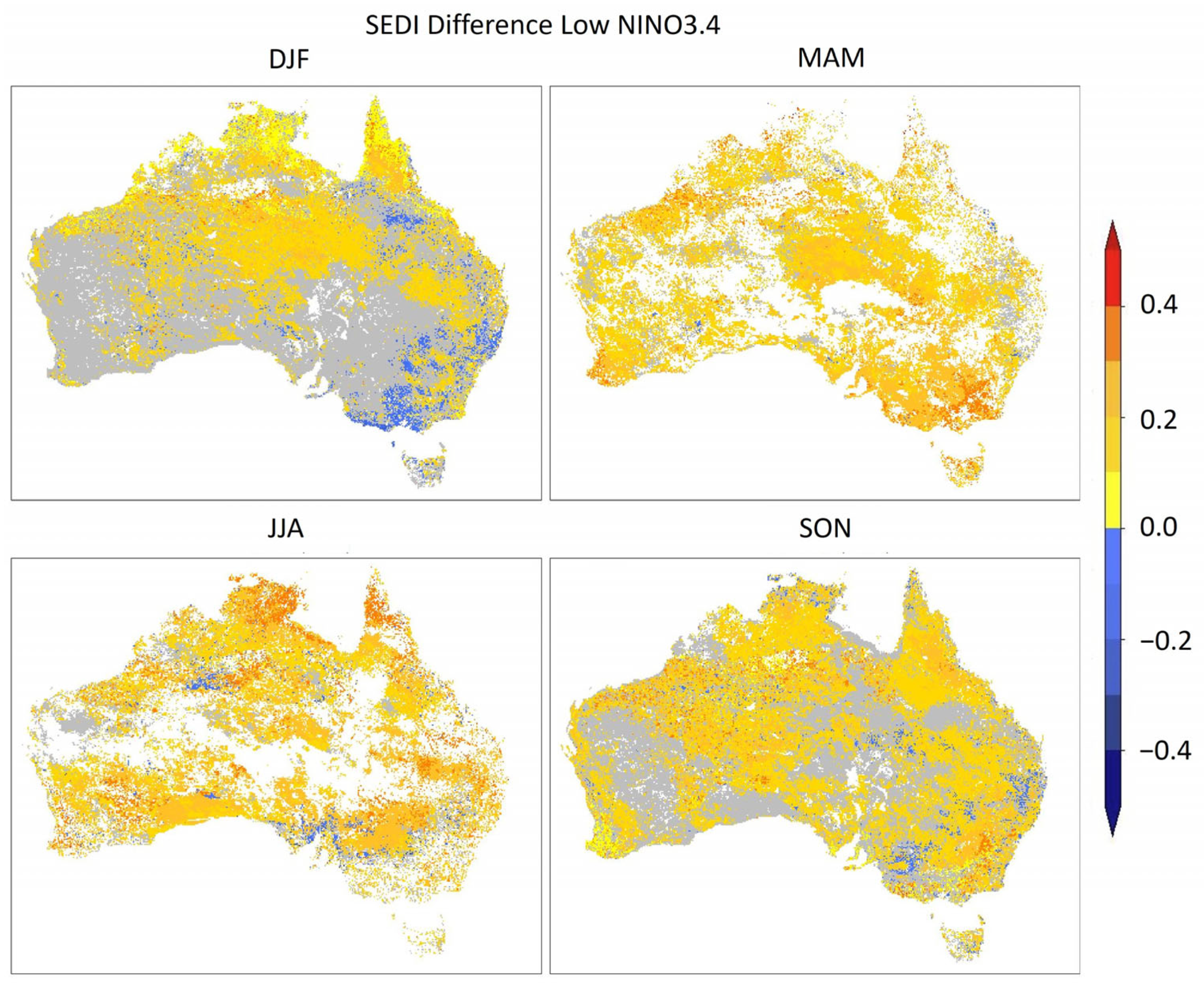
3.2. Prediction Associated with ENSO

Episodes of El Niño increase the predictive skill of ACCESS-S2 over much of Australia in DJF (Figure 2). Importantly, these increases in SEDI skill scores coincide with areas where El Niño is associated with increased chances of extreme FBI, including the far north and parts of southeast Australia. These areas of improved skill are most aligned with observed increased chances of top-decile FBI, but some similarities to the modelled results are also present [46]. In MAM, there are increases in the SEDI scores over most of Australia when an El Niño phase is active. This is noteworthy, given the autumn predictability barrier often confounds the modelling of ENSO and its impacts in MAM. There is a marked decrease in predictive skill in southwest Western Australia (WA) and in inland NSW. However, throughout the hindcast period in this season, El Niño is associated with an increase in fire danger only in the northern reaches of Australia [38], so El Niño may not be an important driver for predicting periods of extreme FBI in southwest Australia and inland NSW in autumn. Conversely, prediction skill in southwest WA shows a strong response to El Niño in JJA and SON, associated with an overall increase in SEDI score compared with the neutral case. An exception occurs in JJA, with a slight decrease in predictive skill in southeast Australia when El Niño is active, which coincides with an area where a stronger-than-observed increase in the chance of extreme FBI is simulated by the model [46]. Increases in skill are generally observed elsewhere across the continent. In SON, there is again a general increase in SEDI scores, especially in the regions where increased probabilities of extreme FBI are observed and simulated in association with El Niño [46]. This is expected, given the pronounced impact of El Niño on rainfall and temperatures in SON, and the active fire danger usually present in Southern Australia during this season [39,40]. It also provides end users of FBI forecasts with additional confidence in the forecasts when an El Niño is active or forecast. Observed increases in Southern Australian fire danger associated with climate change in spring are projected to continue, making fire danger prediction and preparedness particularly important in this season [1,2,40,47]. Additionally, an expected trend towards more frequent and intense El Niño events under climate change conditions [48] highlights the potential usefulness of this driver as a predictive factor now and into the future.

La Niña events are generally associated with increased predictive skill where sufficient data are available to reach significance at the p < 0.10 level (Figure 3). However, the limited sample size discussed by Taylor et al. [46] causes clear limitations in the results for MAM and JJA. This is not altogether unexpected, as ENSO typically transitions in autumn, so a lack of events > 1 SD from the mean is understandable. In DJF, La Niña events result in increased predictive skill in the central and northern regions of Australia but are associated with decreases in skill in the southeast. Increased skill is associated with higher chances of extreme FBI in the central and western desert areas, and the decreases in the southeast are in regions that are neither observed nor simulated to typically experience elevated chances of extreme FBI during La Niña events [46]. Little conclusive evidence can be drawn from the results in MAM due to the limited sample size causing obvious errors in the effect of La Niña on fire danger [40,47]. In JJA, there are also limitations as mentioned, however, the increases in predictive skill in the Arnhem Land and Cape York Peninsula regions are encouraging, given that JJA is a season of active fire danger in the tropics, which may be affected by increased fuel loads during La Niña events. Persistent increases in predictive capacity are observed in SON when a La Niña is present, including in the western desert and southwest, where La Niña is associated with slight increases in the chance of extreme FBI, both in observations and simulations [16,46].

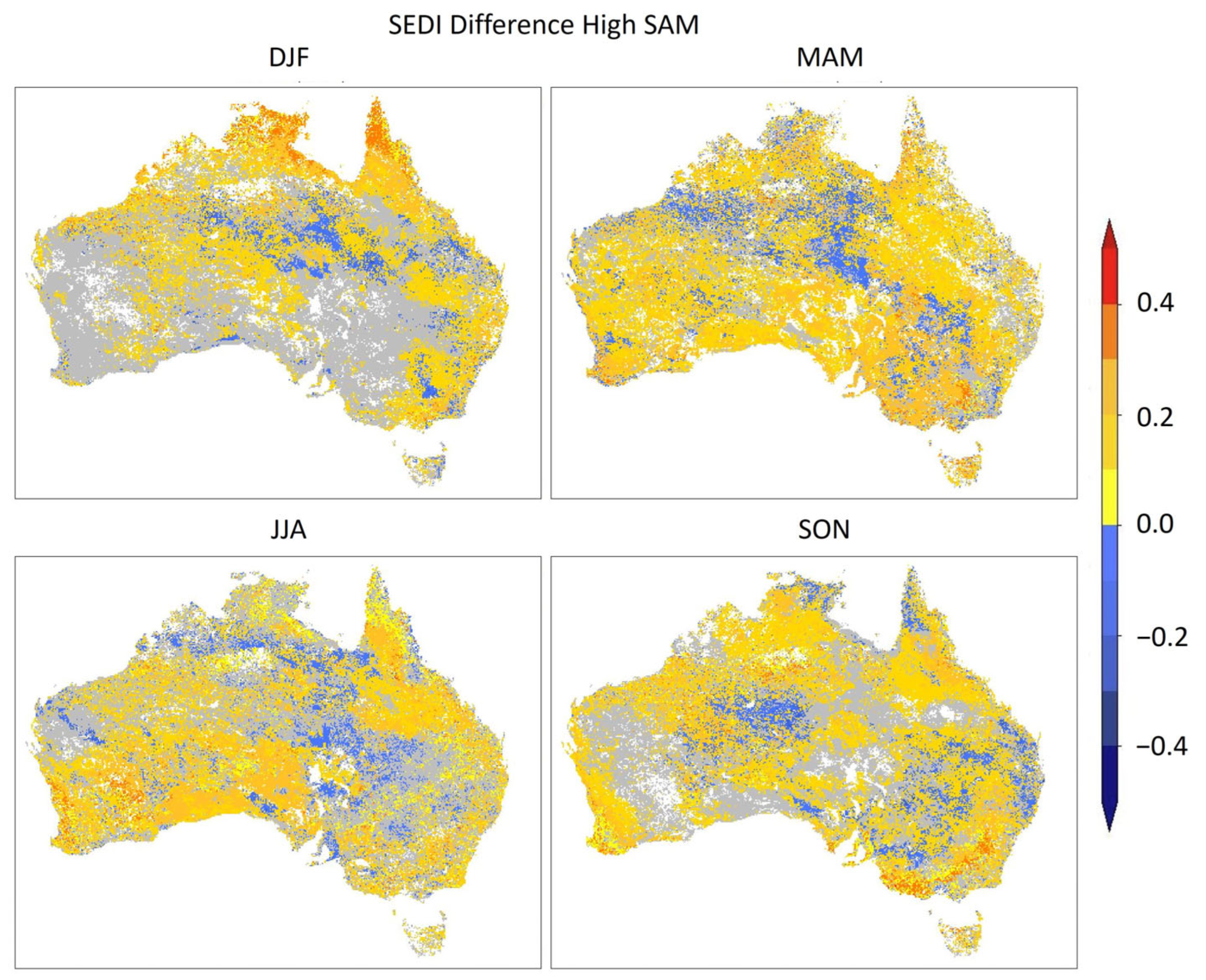
3.3. Prediction Associated with the SAM

Positive SAM events are associated with an overall increase in predictive capacity in northeast and southwest Australia, with decreased accuracy in much of inland Australia and the northern desert regions. The positive SAM (Figure 4) is associated with a lower chance of extreme FBI overall, particularly in ACCESS-S2 simulations, with only slight increases seen in some parts of Northern Australia [46], so the reduced predictive capacity in some parts of inland Australia is unlikely to have negative consequences for end users considering management decisions in light of FBI forecasts. Consistent with understanding [49], increases in predictive skill are available across most of Australia in the negative phase of the SAM (Figure 5) when event likelihood is increased in southern and southeast Australia due to reduced rainfall [49]. This shows the potential for the negative SAM to be an important predictor for forecasting fire season severity in Southern Australia, and greater confidence can be placed in the accuracy of FBI forecasts when this phase is active.

3.4. Prediction Associated with the IOD

Predictive skill is improved across Australia when the IOD is positive in JJA (Figure 6), which is associated with lower rainfall and increased chance of extreme FBI over most of the country. This phase stands out as the most influential climate driver for increasing the chance of top-decile FBI in JJA in some parts of Australia [46], so the high skill of ACCESS-S2 in predicting extreme fire danger in association with the positive IOD is important for decision-making and for understanding FBI forecasts. Slightly lower skill is available in SON, with still predominantly positive SEDI score differences overall. Less skilful forecasts have been available for the negative phase in either season (Figure 7), due to an impaired ability of ACCESS-S2 to capture the magnitude and footprint of the changes in event probability associated with the IOD [46]. Caution is therefore warranted when interpreting FBI forecasts, particularly in negative IOD events, as historically, this has produced inaccurate results in Central and Eastern Australia in JJA, and areas of southeast, southwest and Northern Australia in SON.

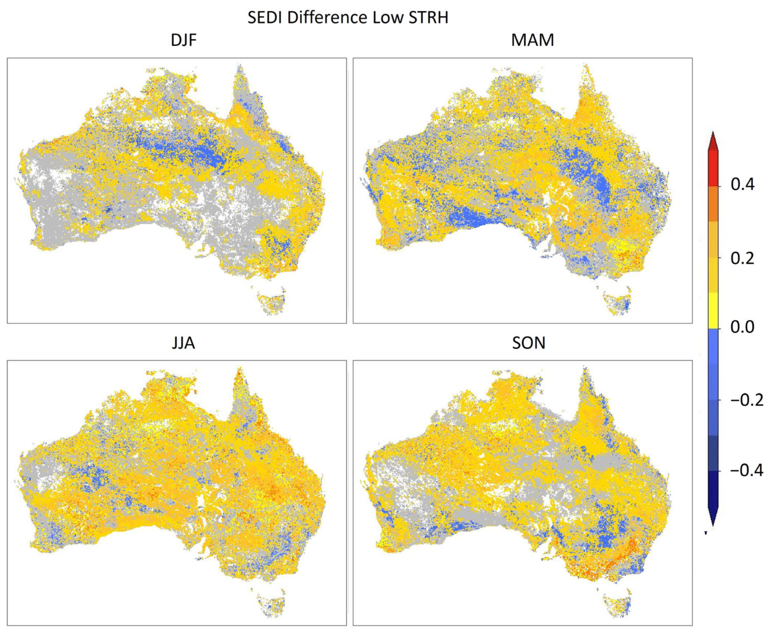
3.5. Prediction Associated with the STRH

In both phases of the STRH and in all seasons, ACCESS-S2 shows mixed ability to predict associated probabilities of extreme FBI. Most instances of observed and simulated high probability of upper-decile FBI associated with positive STRH, importantly in the north [46], correspond with areas of increased forecasting skill (Figure 8) compared with when all available forecasts are used. This improved prediction is particularly evident in the Cape York region, where positive STRH is consistently associated with higher fire danger. Consistent increases in forecasting capacity are evident in Tasmania as well, where aridity and warm air advection result in an increased likelihood of extreme FBI in all seasons [46]. These results show potential for increased confidence in FBI forecasts in Northern Australia and Tasmania when the STRH is positive. The positive results are not sustained in the low phase of the STRH (Figure 9), with ACCESS-S2 showing a decreased ability to predict the observed increased probability of extreme fire danger in Eastern and southeastern Australia. Despite ACCESS-S2 quite accurately reproducing the observed effects of negative STRH events on extreme fire danger in DJF, MAM and SON [46], there are minor differences in the magnitude or exact spatial footprint of the probability ratios, which cause compromised forecast skill. Improvements to known biases in geopotential height representations by ACCESS-S2 may improve the predictive skill associated with negative STRH.

3.6. Prediction Associated with Split-Flow Blocking

Low sampling compromises analysis of the predictive skill associated with key seasons and phases of the BI (Figure 10). This is unfortunate, as ACCESS-S2 does simulate the observed probability ratios with reasonable accuracy in the key seasons of DJF and SON, when the positive BI is associated with high fire danger in some regions of Australia [46]. Where sufficient samples are available, there is a clear increase in predictive skill associated with this mode, with the exception of southwest Western Australia and some of the northern desert region in MAM. These increases in skill capture a low probability of extreme FBI, along with the elevated probability ratios evident along the coastal margin of Northern Australia. In the negative phase of blocking (Figure 11), increased skill is available in most regions where enough data are available. This includes some prominent cases of increased event probability, such as in central and southeast Australia in DJF, central Australia in MAM, the south in JJA and the north and southeast in SON. However, it may be premature to assume greater confidence can be placed in FBI forecasts when the split-flow blocking is active, as the low sampling indicates that they are likely based on very few instances of both observed and simulated fire danger being above the 90th percentile when the negative BI is active. As longer datasets become available, it will become apparent whether this increased forecasting skill is maintained, and whether similar skill is found for the areas without data.

3.7. Prediction Associated with the Madden-Julian Oscillation

The MJO is known to have impacts on Australian climate across the continent and in all phases and seasons [16,27,50]. However, phases highlighted by Taylor et al. [46] have been shown to have particularly strong relationships with chances of extreme FBI over specific areas of interest. Those same phases have been featured here due to their relevance to potential end users of FBI forecasts and outlooks.

Predictive skill for all phases of the MJO in DJF is consistently high across Northern Australia and the East Coast, with little significant data coverage in the south, where fire danger is usually highest in summer. In phase 6 (Figure 12), there is an increase in predictive skill in southeast Australia, some of which overlaps with an observed and modelled increased frequency of extreme FBI [46]. Predictive skill is also much increased in the Cape York Peninsula and the northern interior. Although the decreased probability of extreme FBI is observed and modelled in the Cape York Peninsula region in this phase, increased probabilities are found elsewhere where predictive skill is also high, including central Australia, central Queensland and areas of the southeast [46]. Areas of low predictive skill are evident, particularly in parts of the northern desert and the coast of the Gulf of Carpentaria. In the Gulf of Carpentaria, both observations and models suggest a below-average probability of extreme FBI in phase 6, although the model shows a greater extent of high probability ratios extending through central Queensland and reaching the Gulf regions. In the northern desert region, there are slight discrepancies in the exact distribution and magnitude of increased probability ratios, so while the model may forecast a higher risk of extreme FBI in these areas in MJO phase 6 [46], the historical accuracy of these forecasts has been low. In these instances, stakeholders should carefully consider forecasts for other climate drivers where historical accuracy has been higher, such as the DMI (Figure 6 and Figure 7).

In MAM, phase 6 (Figure 12) has been associated with a large increase in observed frequency of extreme FBI, especially in Southern and Western Australia, where MAM is an active fire season. Notably, ACCESS-S2 shows an enhanced ability to predict extreme FBI in phase 6, with improvements evident in southeast Australia and much of Western Australia, where the probability of extreme FBI is elevated [46]. However, data coverage is not fully complete across Southern Australia, so result reliability in this region is compromised. This is particularly concerning, given the difference between observed and simulated probability of extreme FBI found by Taylor et al. [46], which could be expected to reduce forecast skill in Southern Australia and the Bight region.

In JJA, phase 2 (Figure 12) of the MJO is relevant for forecasting the chance of extreme FBI, as a higher frequency of extreme FBI events is observed across much of Northern Australia where JJA is the dry season [46]. Phase 2 in this season is associated with enhanced convection over Africa and the Indian Ocean, with higher geopotential height over Eastern Australia but increased maximum and minimum temperatures in parts of Northern Australia [24,50]. In the northern desert/southern Cape York regions where maximum temperature is found to increase in phase 2, ACCESS-S2 shows decreased predictive skill for forecasting extreme FBI. Conversely, higher skill is evident in Arnhem land and the east coast of the Cape York Peninsula. This indicates that ACCESS-S2 may not adequately simulate the effect of MJO phase 2 on maximum temperature, introducing additional uncertainty to FBI forecasts when this phase is active.

Phase 3 (Figure 12) is a critical phase for extreme FBI events in SON. Maximum and minimum temperatures coincide with decreased rainfall in southeast Australia [24,27], which would be expected to drive high FBI in the active fire season. SEDI scores for predicted extreme FBI in southeast Australia are lower than climatology for this phase. Although ACCESS-S2 shows improved skill for the southernmost coast, a large region of inland southeast Australia has decreased predictive skill. Surprisingly, the observed likelihood of extreme FBI in this region is lower than what is simulated [46]. This difference does not indicate a lack of skill in the model’s representation of phase 3 impacts, but may rather be due to the short FBI record and an inadequate representation of phase 2 events in the SON dataset. Regardless of the cause, these results show that MJO phase 3 does not play a key role in providing predictive skill in this region, and the activity of other climate drivers should be carefully considered.

4. Synthesis

In this study, we have used the SEDI skill score for extreme events to depict the accuracy with which episodes of top-decile FBI can be predicted 2–3 weeks ahead from climate driver modes using the Bureau of Meteorology subseasonal-to-seasonal climate model, ACCESS-S2. This investigation holds importance beyond evaluating the predictive performance of ACCESS-S2; it also demonstrates the role that each climate driver has in providing subseasonal predictive skill for extreme FBI across Australia in the current prediction system. By understanding these roles in conjunction with known relationships with FBI [46] and the skill of ACCESS-S2 in predicting key climate drivers [22], we are able to better understand the model’s strengths and weaknesses. Further, we can demonstrate how these translate to areas of improved forecast skill at subseasonal timescales. This is relevant for developing both the AFDRS and the ACCESS-S prediction system. The results show that all active drivers provide additional skill to FBI forecasts in some seasons and regions, based on historical forecast accuracy in time when the driver has been in its active phase. In areas where added forecast skill is available during the fire season, knowledge of the activities of these drivers may aid regional end users in various decisions, knowing whether increased confidence can be placed in official FBI forecasts. This would be over and above the high confidence, which is already evident from the high SEDI scores available regardless of climate driver activity (Figure 1).

In DJF, much of south and southeast Australia experiences its highest fire danger. In the southwest, good skill is available in forecasts when La Niña, positive STRH or negative BI is active, as well as either phase of the SAM. For southeast Australia, including Tasmania, where fire danger is typically at a maximum in DJF, skill is added to FBI forecasts in episodes of La Niña, positive and negative SAM, negative STRH, low blocking and phases 3–8 of the MJO. In phases 1 and 2 of the MJO and during high split-flow blocking, insufficient data are available to make confident skill assessments (

Table 2. Synthesis of driver predictive skill for DJF by geographic quadrant. Key applies for Table 2, Table 3, Table 4 and Table 5.

DJF	Geographic quadrant				Predictive Skill Key
Driver	NE	SE	SW	NW	Excellent (SEDI difference > 0.50)
NINO3.4+
NINO3.4−					Good (SEDI difference 0.40–0.50)
SAM+
SAM−					Fair/mixed (SEDI difference 0.30–0.40)
STRH+
STRH−					Predominently low/insufficient data (SEDI difference > 0.30)
BI+
BI−
MJO phase 6

).

MAM is also often a period of high fire risk in Southern Australia. In this season, added skill is available in the southeast and the Bight during El Niño, the SAM, high blocking and phases 4–8 of the MJO. Other drivers tend to be associated with considerable areas of land where forecast accuracy is lower than climatology when the driver is active (

Table 3. Synthesis of driver predictive skill for MAM by geographic quadrant.

MAM	Geographic quadrant				Predictive Skill Key
Driver	NE	SE	SW	NW	Excellent (SEDI difference > 0.50)
NINO3.4+
NINO3.4−					Good (SEDI difference 0.40–0.50)
SAM+
SAM−					Fair/mixed (SEDI difference 0.30–0.40)
STRH+
STRH−					Predominently low/insufficient data (SEDI difference > 0.30)
BI+
BI−
MJO phase 6

). The southwest shows a similar response, with the exception of positive BI and phases 6 and 8 of the MJO. However, isolated regions in the southwest, generally the coastal tip, experience added forecast skill in other times as well.

In JJA, fire danger generally peaks in Northern Australia, where this is the dry season. Very high forecast skill is typically available in Northern Australia in this season, but it is increased beyond climatology during both high and low SAM, positive IOD, negative STRH, high blocking and phase 5 of the MJO. La Niña and low blocking episodes, as well as phases, 3, 4, 6 and 7 of the MJO, may also have added skill but the sampling is generally too sparse to draw confident conclusions (

Table 4. Synthesis of driver predictive skill for JJA by geographic quadrant.

JJA	Geographic quadrant
Driver	NE	SE	SW	NW
NINO3.4+					Predictive Skill Key
NINO3.4−					Excellent (SEDI difference > 0.50)
SAM+
SAM−					Good (SEDI difference 0.40–0.50)
IOD+
IOD−					Fair/mixed (SEDI difference 0.30–0.40)
STRH+
STRH−					Predominently low/insufficient data (SEDI difference > 0.30)
BI+
BI−
MJO phase 2

).

SON is the season of active fire danger for the largest area of Australia, with fire danger potentially peaking from northern through central Australia, and fire danger rising over time in Southern Australia as well. Across northern and central Australia, forecast accuracy has historically increased broadly in periods of La Niña, positive SAM, negative STRH and MJO phases 2, 3 and 5. La Niña, positive and negative SAM and the aforementioned phases of the MJO are also influential for increasing forecast accuracy in Southern Australia, while additionally, MJO phases 2, 6 and 8 provide notable improvements in skill. In other driver phases, increases in skill are mixed or discontinuous (

Table 5. Synthesis of driver predictive skill for SON by geographic quadrant.

SON	Geographic quadrant
Driver	NE	SE	SW	NW
NINO3.4+					Predictive Skill Key
NINO3.4−					Excellent (SEDI difference > 0.50)
SAM+
SAM−					Good (SEDI difference 0.40–0.50)
IOD+
IOD−					Fair/mixed (SEDI difference 0.30–0.40)
STRH+
STRH−					Predominently low/insufficient data (SEDI difference > 0.30)
BI+
BI−
MJO phase 3

). The skill added from the MJO is particularly encouraging, given the strong influence the MJO is known to have on rainfall, temperature and fire danger in these phases and seasons [16,24,27,46].

In addition to these areas of increased skill, parts of the continent show lower predictive skill in certain climate driver modes. These include El Niño in DJF and MAM, positive SAM, negative IOD and the positive (March–November) and negative (DJF, MAM, SON) phases of the STRH (Table 2, Table 3, Table 4 and Table 5). These areas where skill is reduced compared with climatology highlight occasions where the model inadequately captures the observed impact of the subseasonal climate on FBI [46]. This could be related to biases and systematic errors in the model (e.g., [22]). Alternatively, some mismatches between modelled and observed FBI-climate relationships could be the result of the short hindcast period, which may not encompass sufficient events to reliably demonstrate the long-term average impact of these climate driver states. Revisiting these relationships in the future may resolve this issue, making it possible to determine where model biases are affecting forecast skill, and highlighting areas for continued development and investigation in future iterations of the forecasting system.

5. Concluding Remarks

The areas of increased hindcast skill for predicting high FBI indicate that several of the major drivers of Australian weather and climate have been associated with greater accuracy in FBI outlooks. The current FBI seasonal outlook system using ACCESS-S2 has been operational since March 2023 and will equally be affected by these changes in forecast skill. Therefore, the results shown in this paper may be valuable for regional end users whose decision-making may be affected by fire danger outlooks, including those in national park and forest estate management, agriculture, emergency services, health and energy. By combining seasonal FBI outlooks with climate driver forecasts, the Bureau of Meteorology may have the capacity to provide a greater wealth of information and greater confidence to users relying on FBI outlooks for key management decisions.

References

1. Clarke, H.; Lucas, C.; Smith, P. Changes in Australian fire weather between 1973 and 2010. Int. J. Climatol. 2013, 33, 931–944. [Google Scholar] [CrossRef]
2. Dowdy, A.J. Climatological Variability of Fire Weather in Australia. J. Appl. Meteorol. Climatol. 2018, 57, 221–234. [Google Scholar] [CrossRef]
3. Commonwealth of Australia. A Nation Charred: Report on the Inquiry into Bushfires; Nairn, G., Ed.; Commonwealth of Australia: Canberra, Australia, 2003.
4. Teague, B.; Pascoe, S.; McLeod, R. The 2009 Victorian Bushfires Royal Commission Final Report: Summary; Parliament of Victoria: Melbourne, Australia, 2010.
5. Filkov, A.I.; Ngo, T.; Matthews, S.; Telfer, S.; Penman, T.D. Impact of Australia’s catastrophic 2019/20 bushfire season on communities and environment. Retrospective analysis and current trends. J. Saf. Sci. Resil. 2020, 1, 44–56. [Google Scholar] [CrossRef]
6. Moreira, F.; Ascoli, D.; Safford, H.; Adams, M.A.; Moreno, J.M.; Pereira, J.M.; Catry, F.X.; Armesto, J.; Bond, W.; González, M.E.; et al. Wildfire management in Mediterranean-type regions: Paradigm change needed. Environ. Res. Lett. 2020, 15, 011001. [Google Scholar] [CrossRef]
7. Moritz, M.A.; Batllori, E.; Bradstock, R.A.; Gill, A.M.; Handmer, J.; Hessburg, P.F.; Leonard, J.; McCaffrey, S.; Odion, D.C.; Schoennagel, T.; et al. Learning to coexist with wildfire. Nature 2014, 515, 58–66. [Google Scholar] [CrossRef]
8. Nolan, R.H.; Bowman, D.M.; Clarke, H.; Haynes, K.; Ooi, M.K.; Price, O.F.; Williamson, G.J.; Whittaker, J.; Bedward, M.; Boer, M.M. What Do the Australian Black Summer Fires Signify for the Global Fire Crisis? Fire 2021, 4, 97. [Google Scholar] [CrossRef]
9. Iwakiri, T.; Imada, Y.; Takaya, Y.; Kataoka, T.; Tatebe, H.; Watanabe, M. Triple-Dip La Niña in 2020–23: North Pacific Atmosphere Drives 2nd Year La Niña. Geophys. Res. Lett. 2023, 50, e2023GL105763. [Google Scholar] [CrossRef]
10. O’Donnell, A.J.; Boer, M.M.; McCaw, W.L.; Grierson, P.F. Climatic anomalies drive wildfire occurrence and extent in semi-arid shrublands and woodlands of southwest Australia. Ecosphere 2011, 2, 1–15. [Google Scholar] [CrossRef]
11. Letnic, M.; Dickman, C.R. Boom Means Bust: Interactions between the El Niño/Southern Oscillation (ENSO), Rainfall and the Processes Threatening Mammal Species in Arid Australia. Biodivers. Conserv. 2006, 15, 3847–3880. [Google Scholar] [CrossRef]
12. Bureau of Meteorology. Climate Outlooks. 31 August 2023. Available online: http://www.bom.gov.au/climate/outlooks/#/overview/summary (accessed on 5 September 2023).
13. Bureau of Meteorology. Australian Rainfall during El Niño and La Niña Events. 2023. Available online: http://www.bom.gov.au/climate/history/enso/ (accessed on 14 December 2023).
14. Palmer, J.G.; Cook, E.R.; Turney, C.S.; Allen, K.; Fenwick, P.; Cook, B.I.; O’Donnell, A.; Lough, J.; Grierson, P.; Baker, P. Drought variability in the eastern Australia and New Zealand summer drought atlas (ANZDA, CE 1500–2012) modulated by the Interdecadal Pacific Oscillation. Environ. Res. Lett. 2015, 10, 124002. [Google Scholar] [CrossRef]
15. Biskin, M.; Bennett, A.; Macintosh, A. Chapter 17: Public and private land management. In Royal Commission into National Natural Disaster Arrangements Report; Commonwealth of Australia: Canberra, Australia, 2020. [Google Scholar]
16. Marshall, A.G.; Gregory, P.A.; de Burgh-Day, C.O.; Griffiths, M. Subseasonal drivers of extreme fire weather in Australia and its prediction in ACCESS-S1 during spring and summer. Clim. Dyn. 2021, 58, 523–553. [Google Scholar] [CrossRef]
17. McArthur, A.G. Fire Behaviour in Eucalypt Forests; Commonwealth of Australia: Canberra, Australia, 1967.
18. Matthews, S. Fire Behaviour Index Technical Guide. 2022. Available online: https://www.afac.com.au/initiative/afdrs/technical-resources (accessed on 3 August 2023).
19. Matthews, S.; Fox-Hughes, P.; Grootemaat, S.; Hollis, J.J.; Kenny, B.J.; Sauvage, S. Australian Fire Danger Rating System: Research Prototype; NSW Rural Fire Service: Lidcombe, Australia, 2019.
20. Australian Bureau of Meteorology. Bureau of Meteorology Fire Behaviour Model Guides. 2022. Available online: https://www.afac.com.au/initiative/afdrs/article/bom-fire-behaviour-model-guides (accessed on 3 August 2023).
21. Fox-Hughes, P.; Benger, N.; Gregory, P. AFAC Conference: Report: Progress towards a new national seasonal fire outlook. Aust. J. Emerg. Manag. 2022, 37, 59–62. [Google Scholar]
22. Wedd, R.; Alves, O.; de Burgh-Day, C.; Down, C.; Griffiths, M.; Hendon, H.H.; Hudson, D.; Li, S.; Lim, E.P.; Marshall, A.G.; et al. ACCESS-S2: The upgraded Bureau of Meteorology multi-week to seasonal prediction system. J. South. Hemisph. Earth Syst. Sci. 2022, 72, 218–242. [Google Scholar] [CrossRef]
23. Marshall, A.G.; Hudson, D.; Wheeler, M.C.; Alves, O.; Hendon, H.H.; Pook, M.J.; Risbey, J.S. Intra-seasonal drivers of extreme heat over Australia in observations and POAMA-2. Clim. Dyn. 2014, 43, 1915–1937. [Google Scholar] [CrossRef]
24. Marshall, A.G.; Wheeler, M.C.; Cowan, T. Madden-Julian Oscillation Impacts on Australian Temperatures and Extremes. J. Clim. 2023, 36, 335–357. [Google Scholar] [CrossRef]
25. Pook, M.J.; Risbey, J.S.; McIntosh, P.C.; Ummenhofer, C.C.; Marshall, A.G.; Meyers, G.A. The Seasonal Cycle of Blocking and Associated Physical Mechanisms in the Australian Region and Relationship with Rainfall. Mon. Weather Rev. 2013, 141, 4534–4553. [Google Scholar] [CrossRef]
26. Risbey, J.S.; Pook, M.J.; McIntosh, P.C.; Wheeler, M.C.; Hendon, H.H. On the Remote Drivers of Rainfall Variability in Australia. Mon. Weather Rev. 2009, 137, 3233–3253. [Google Scholar] [CrossRef]
27. Cowan, T.; Wheeler, M.; Marshall, A.G. The combined influence of the Madden-Julian Oscillation and El Niño Southern Oscillation on Australian rainfall. J. Clim. 2023, 36, 313–334. [Google Scholar] [CrossRef]
28. Taylor, R.; Marshall, A.G.; Crimp, S.; Cary, G.J.; Harris, S.; Sauvage, S. Associations between Australian climate drivers and extreme weekly fire danger. Int. J. Wildland Fire 2023, 33, WF23060. [Google Scholar] [CrossRef]
29. Kalnay, E.; Kanamitsu, M.; Kistler, R.; Collins, W.; Deaven, D.; Gandin, L.; Iredell, M.; Saha, S.; White, G.; Woollen, J. The NCEP/NCAR 40-year reanalysis project. Bull. Am. Meteorol. Soc. 1996, 77, 437–471. [Google Scholar] [CrossRef]
30. Ferro, C.A.; Stephenson, D.B. Extremal dependence indices: Improved verification measures for deterministic forecasts of rare binary events. Weather Forecast. 2011, 26, 699–713. [Google Scholar] [CrossRef]
31. Magnusson, L.; Haiden, T.; Richardson, D. Verification of Extreme Weather Events: Discrete Predictands; European Centre for Medium-Range Weather Forecasts: Reading, UK, 2014. [Google Scholar]
32. North, R.; Trueman, M.; Mittermaier, M.; Rodwell, M.J. An assessment of the SEEPS and SEDI metrics for the verification of 6 h forecast precipitation accumulations. Meteorol. Appl. 2013, 20, 164–175. [Google Scholar] [CrossRef]
33. Collaboration for Australian Weather and Climate Research. Forecast Verification Issues, Methods and FAQ. In Proceedings of the 7th International Verification Methods Workshop, Berlin, Germany, 8–11 May 2017. [Google Scholar]
34. Wheeler, M.C.; Hendon, H.H. An All-Season Real-Time Multivariate MJO Index: Development of an Index for Monitoring and Prediction. Mon. Weather Rev. 2004, 132, 1917–1932. [Google Scholar] [CrossRef]
35. Trenberth, K.E. The Definition of El Niño. Bull. Am. Meteorol. Soc. 1997, 78, 2771–2778. [Google Scholar] [CrossRef]
36. Saji, N.H.; Yamagata, T. Possible impacts of Indian Ocean Dipole mode events on global climate. Clim. Res. 2003, 25, 151–169. [Google Scholar] [CrossRef]
37. Gong, D.; Wang, S. Definition of Antarctic oscillation index. Geophys. Res. Lett. 1999, 26, 459–462. [Google Scholar] [CrossRef]
38. Pook, M.; Gibson, T. Atmospheric blocking and storm tracks during SOP-1 of the FROST Project. Aust. Meteorol. Mag. 1999, 48, 51–60. [Google Scholar]
39. Bureau of Meteorology. Bushfire Weather. 2022. Available online: http://www.bom.gov.au/weather-services/fire-weather-centre/bushfire-weather/index.shtml (accessed on 20 September 2022).
40. Dowdy, A.J. Seamless climate change projections and seasonal predictions for bushfires in Australia. J. South. Hemisph. Earth Syst. Sci. 2020, 70, 120–138. [Google Scholar] [CrossRef]
41. Clarke, H.; Evans, J.P. Exploring the future change space for fire weather in southeast Australia. Theor. Appl. Climatol. 2018, 136, 513–527. [Google Scholar] [CrossRef]
42. Clarke, H.; Pitman, A.J.; Kala, J.; Carouge, C.; Haverd, V.; Evans, J.P. An investigation of future fuel load and fire weather in Australia. Clim. Change 2016, 139, 591–605. [Google Scholar] [CrossRef]
43. Fox-Hughes, P. Future fire danger climatology for Tasmania, Australia, using a dynamically downscaled regional climate model. Int. J. Wildland Fire 2014, 23, 309–321. [Google Scholar] [CrossRef]
44. Cary, G. Importance of a changing climate for fire regimes in Australia. In Flammable Australia: The Fire Regimes and Biodiversity of a Continent; Cambridge University Press: Cambridge, UK, 2002; pp. 26–46. [Google Scholar]
45. Pitman, A.; Narisma, G.; McAneney, J. The impact of climate change on the risk of forest and grassland fires in Australia. Clim. Chang. 2007, 84, 383–401. [Google Scholar] [CrossRef]
46. Taylor, R.; Marshall, A.G.; Crimp, S.; Harris, S.; Cary, G.J.; Gregory, P. Observed Associations between Fire Danger and Climate Modes and their Representation in ACCESS-S2. J. Appl. Meteorol. Climatol. 2023. submitted. [Google Scholar]
47. Harris, S.; Lucas, C. Understanding the variability of Australian fire weather between 1973 and 2017. PLoS ONE 2019, 14, e0222328. [Google Scholar] [CrossRef] [PubMed]
48. Cai, W.; Santoso, A.; Collins, M.; Dewitte, B.; Karamperidou, C.; Kug, J.S.; Lengaigne, M.; McPhaden, M.J.; Stuecker, M.F.; Taschetto, A.S.; et al. Changing El Niño–Southern Oscillation in a warming climate. Nat. Rev. Earth Environ. 2021, 2, 628–644. [Google Scholar] [CrossRef]
49. Hendon, H.H.; Thompson, D.W.J.; Wheeler, M.C. Australian Rainfall and Surface Temperature Variations Associated with the Southern Hemisphere Annular Mode. J. Clim. 2007, 20, 2452–2467. [Google Scholar] [CrossRef]
50. Marshall, A.G.; Wang, G.M.; Hendon, H.H.; Lin, H. Madden-Julian Oscillation teleconnections to Australian springtime temperature extremes and their prediction in ACCESS-S1. Clim. Dyn. 2023, 61, 431–447. [Google Scholar] [CrossRef]
Figure 1. SEDI skill scores for ACCESS-S2 forecasts of upper decile weekly FBI events in DJF (top left), MAM (top right), JJA (lower left) and SON (lower right) at target lead times of weeks 2 and 3 combined using all available forecasts (i.e., not stratified by climate driver or phase). Grey areas indicate where skill scores are not significantly different from zero at 90% confidence using SEDI standard error.
Atmosphere 15 00203 g001
Figure 2. SEDI skill scores for ACCESS-S2 forecasts of upper decile weekly FBI events in periods of high NINO3.4 index in DJF (top left), MAM (top right), JJA (lower left) and SON (lower right) at target lead times of weeks 2 and 3 combined, shown as differences from when all available forecasts are used (Figure 1). Grey areas indicate where skill scores are not significantly different from zero at 90% confidence using SEDI standard error.
Atmosphere 15 00203 g002
Figure 3. SEDI skill scores for ACCESS-S2 forecasts of upper decile weekly FBI events in periods of low NINO3.4 index in DJF (top left), MAM (top right), JJA (lower left) and SON (lower right) at target lead times of weeks 2 and 3 combined, shown as differences from when all available forecasts are used (Figure 1). Grey areas indicate where skill scores are not significantly different from zero at 90% confidence using SEDI standard error.
Atmosphere 15 00203 g003
Figure 4. SEDI skill scores for ACCESS-S2 forecasts of upper decile weekly FBI events in periods of high SAM index in DJF (top left), MAM (top right), JJA (lower left) and SON (lower right) at target lead times of weeks 2 and 3 combined, shown as differences from when all available forecasts are used (Figure 1). Grey areas indicate where skill scores are not significantly different from zero at 90% confidence using SEDI standard error.
Atmosphere 15 00203 g004
Figure 5. SEDI skill scores for ACCESS-S2 forecasts of upper decile weekly FBI events in periods of low SAM index in DJF (top left), MAM (top right), JJA (lower left) and SON (lower right) at target lead times of weeks 2 and 3 combined, shown as differences from when all available forecasts are used (Figure 1). Grey areas indicate where skill scores are not significantly different from zero at 90% confidence using SEDI standard error.
Atmosphere 15 00203 g005
Figure 6. SEDI skill scores for ACCESS-S2 forecasts of upper decile weekly FBI events in periods of high DMI in JJA (left) and SON (right) at target lead times of weeks 2 and 3 combined, shown as differences from when all available forecasts are used (Figure 1). Grey areas indicate where skill scores are not significantly different from zero at 90% confidence using SEDI standard error.
Atmosphere 15 00203 g006
Figure 7. SEDI skill scores for ACCESS-S2 forecasts of upper decile weekly FBI events in periods of low DMI in JJA (left) and SON (right) at target lead times of weeks 2 and 3 combined, shown as differences from when all available forecasts are used (Figure 1). Grey areas indicate where skill scores are not significantly different from zero at 90% confidence using SEDI standard error.
Atmosphere 15 00203 g007
Figure 8. SEDI skill scores for ACCESS-S2 forecasts of upper decile weekly FBI events in periods of high STRH index in DJF (top left), MAM (top right), JJA (lower left) and SON (lower right) at target lead times of weeks 2 and 3 combined, shown as differences from when all available forecasts are used (Figure 1). Grey areas indicate where skill scores are not significantly different from zero at 90% confidence using SEDI standard error.
Atmosphere 15 00203 g008
Figure 9. SEDI skill scores for ACCESS-S2 forecasts of upper decile weekly FBI events in periods of low STRH index in DJF (top left), MAM (top right), JJA (lower left) and SON (lower right) at target lead times of weeks 2 and 3 combined, shown as differences from when all available forecasts are used (Figure 1). Grey areas indicate where skill scores are not significantly different from zero at 90% confidence using SEDI standard error.
Atmosphere 15 00203 g009
Figure 10. SEDI skill scores for ACCESS-S2 forecasts of upper decile weekly FBI events in periods of high BI in DJF (top left), MAM (top right), JJA (lower left) and SON (lower right) at target lead times of weeks 2 and 3 combined, shown as differences from when all available forecasts are used (Figure 1). Grey areas indicate where skill scores are not significantly different from zero at 90% confidence using SEDI standard error.
Atmosphere 15 00203 g010
Figure 11. SEDI skill scores for ACCESS-S2 forecasts of upper decile weekly FBI events in periods of low BI in DJF (top left), MAM (top right), JJA (lower left) and SON (lower right) at target lead times of weeks 2 and 3 combined, shown as differences from when all available forecasts are used (Figure 1). Grey areas indicate where skill scores are not significantly different from zero at 90% confidence using SEDI standard error.
Atmosphere 15 00203 g011
Figure 12. SEDI skill scores for ACCESS-S2 forecasts of upper decile weekly FBI events in periods of MJO phase 6 in DJF (top left) and MAM (top right), phase 2 in JJA (lower left) and phase 3 in SON (lower right) at target lead times of weeks 2 and 3 combined, shown as differences from when all available forecasts are used (Figure 1). Grey areas indicate where skill scores are not significantly different from zero at 90% confidence using SEDI standard error.
Atmosphere 15 00203 g012