
An Improved Deep Learning Approach Considering Spatiotemporal Heterogeneity for PM2.5 Prediction: A Case Study of Xinjiang, China


Abstract
1. Introduction
2. Study Area and Materials
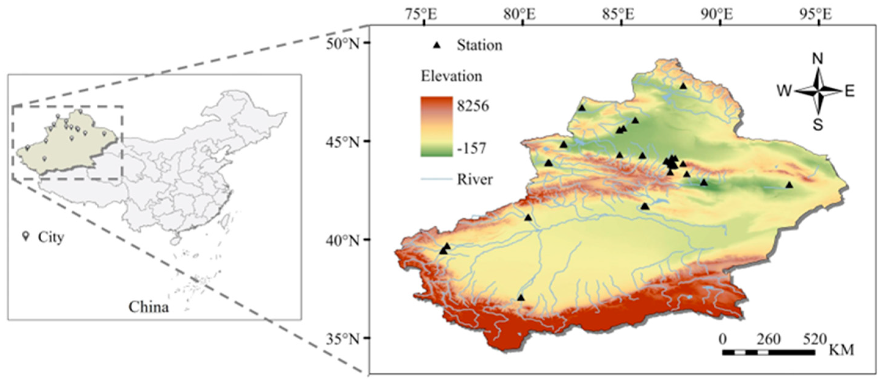
2.1. Study Area
2.2. Data
2.2.1. PM2.5
2.2.2. Feature Variables
2.3. Data Preprocessing
3. Methods
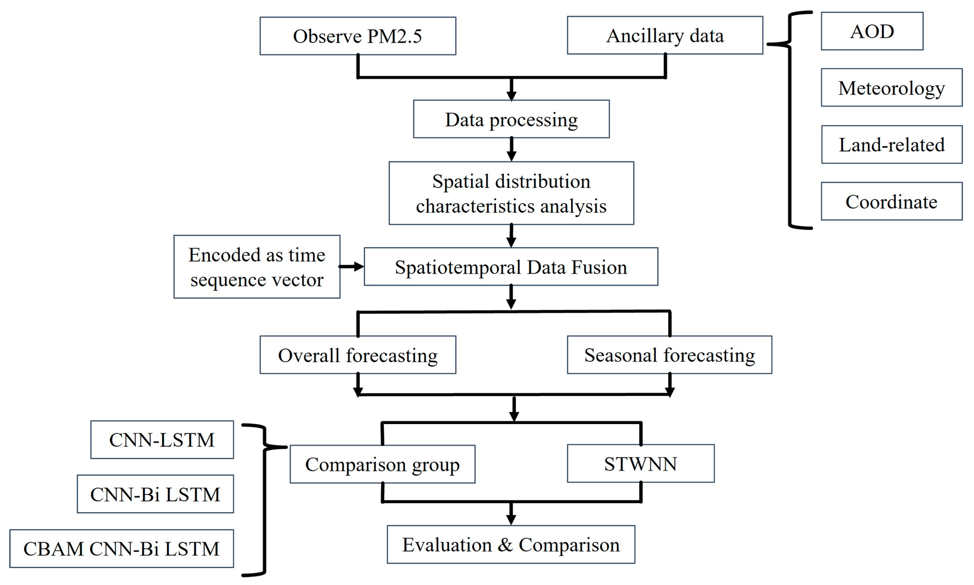
3.1. Flow Chart
3.2. Spatiotemporal Analysis and Clustering
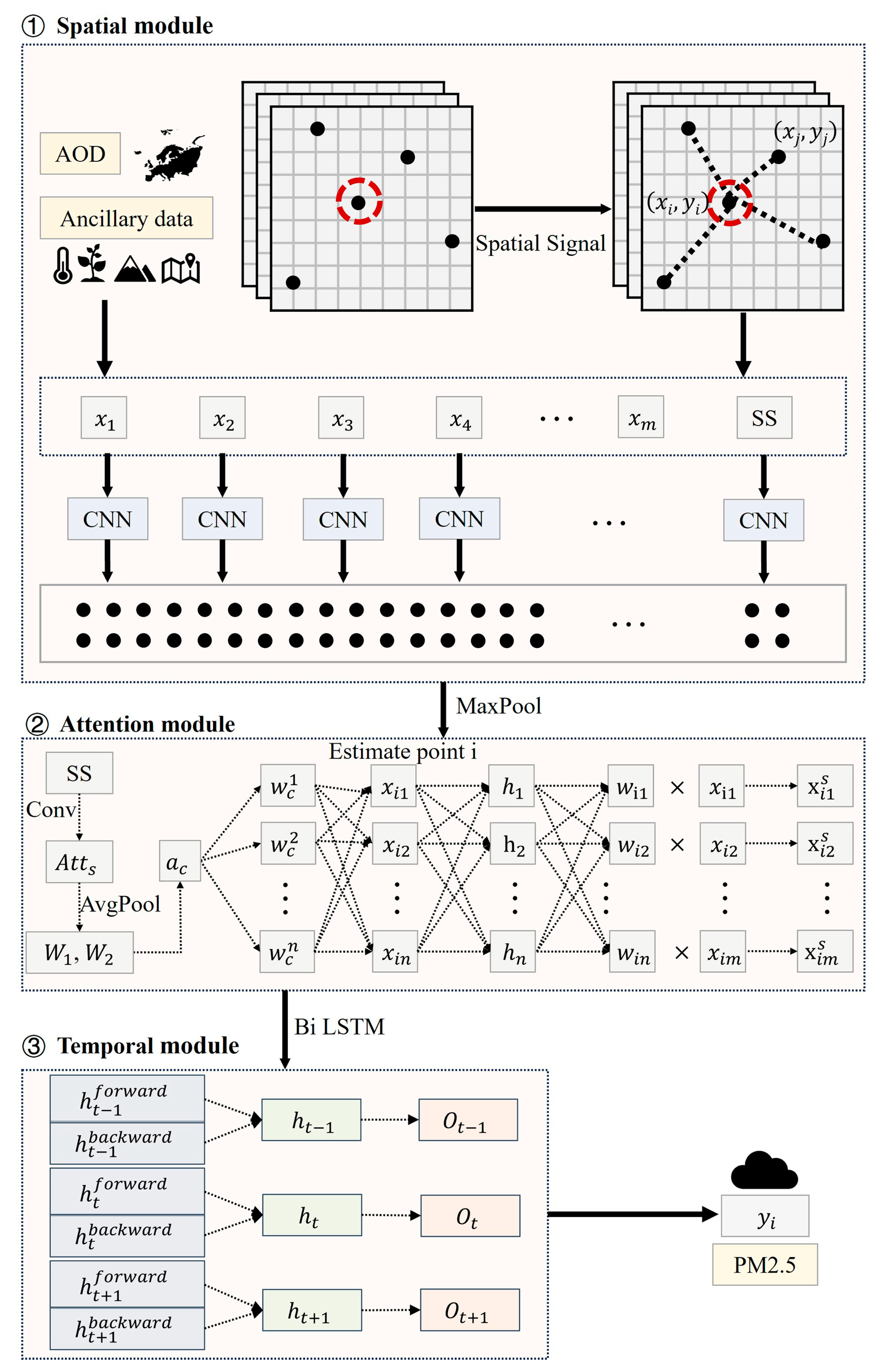
3.3. STWNN
3.3.1. Spatial Module
3.3.2. Attention Module
3.3.3. Temporal Module
3.4. Evaluation Indicators
3.5. Explainability Analysis of Deep Learning Models
4. Results
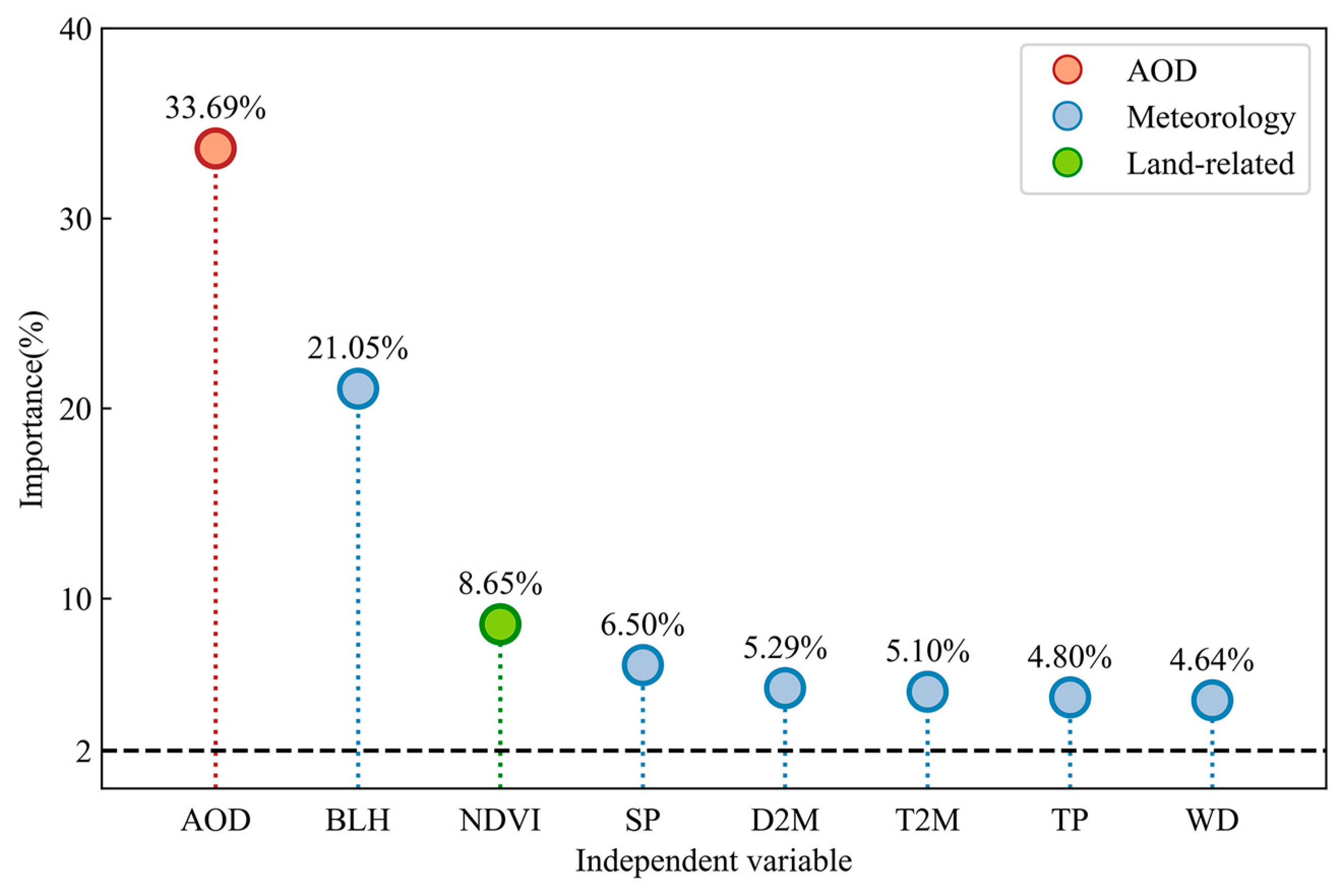
4.1. Variable Importance
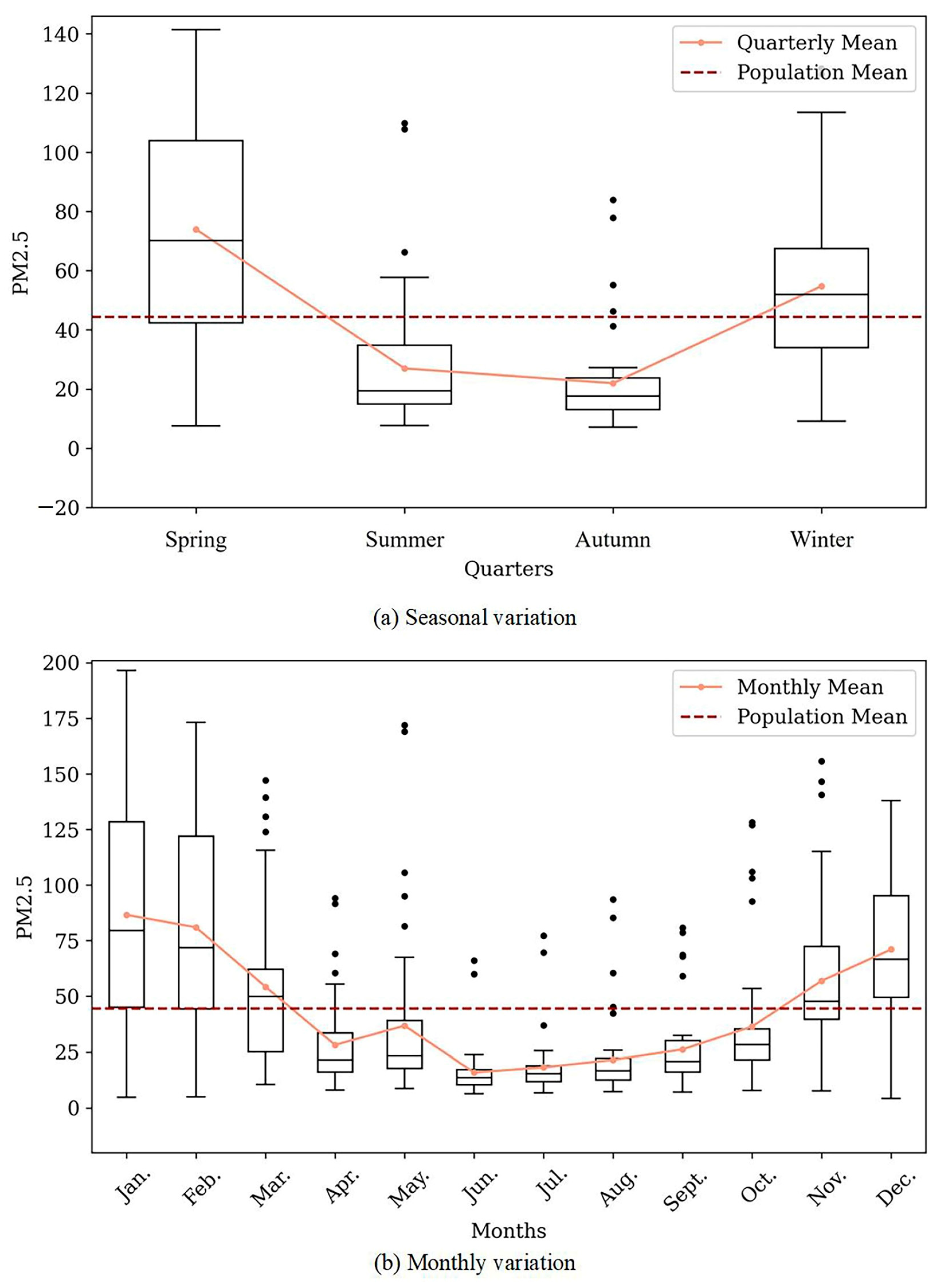
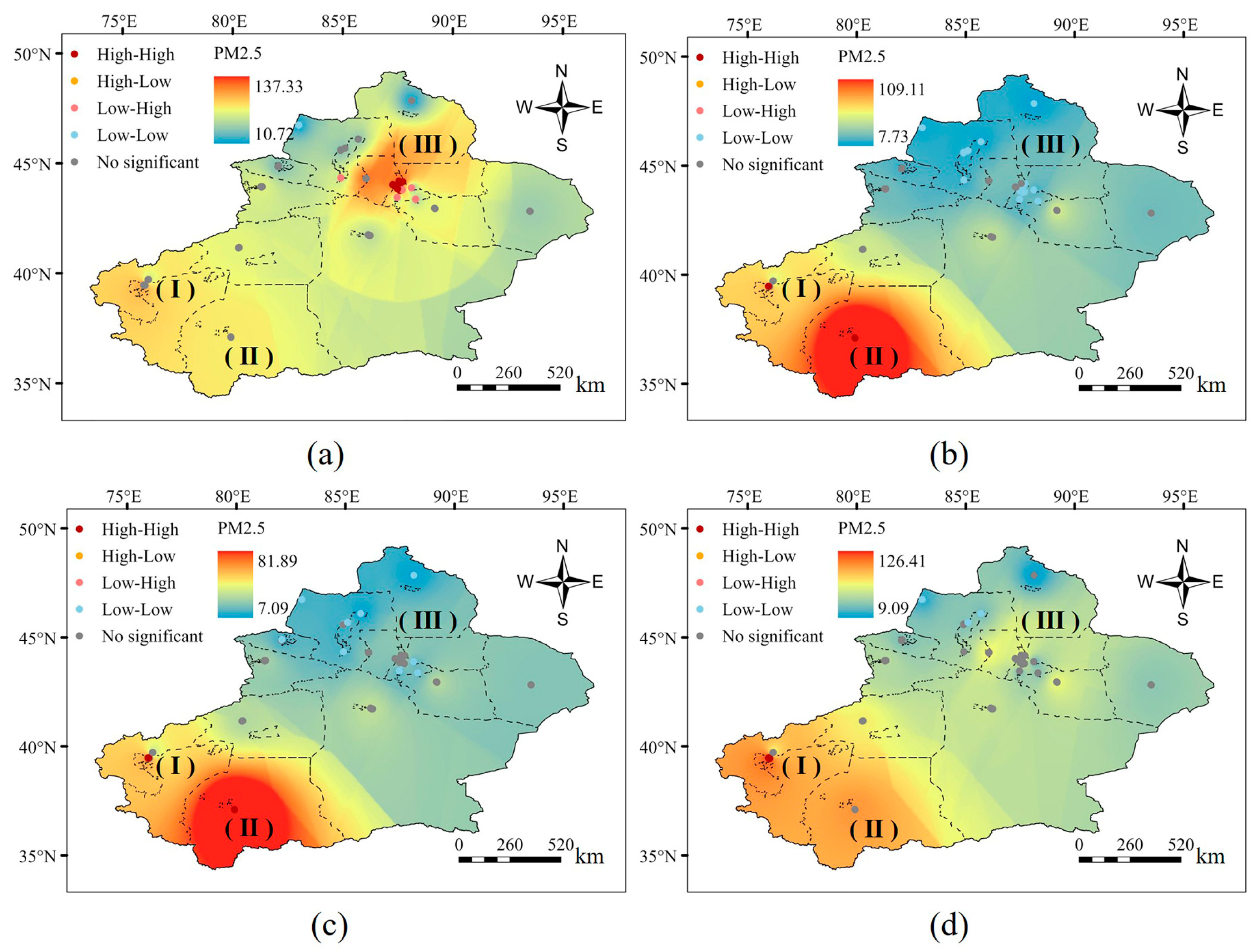
4.2. Characteristics of Spatial and Temporal Distribution of PM2.5
4.3. Model Fitting and Validation
4.3.1. Determination of Proximity Points Number N for SS
4.3.2. Overall Forecasting
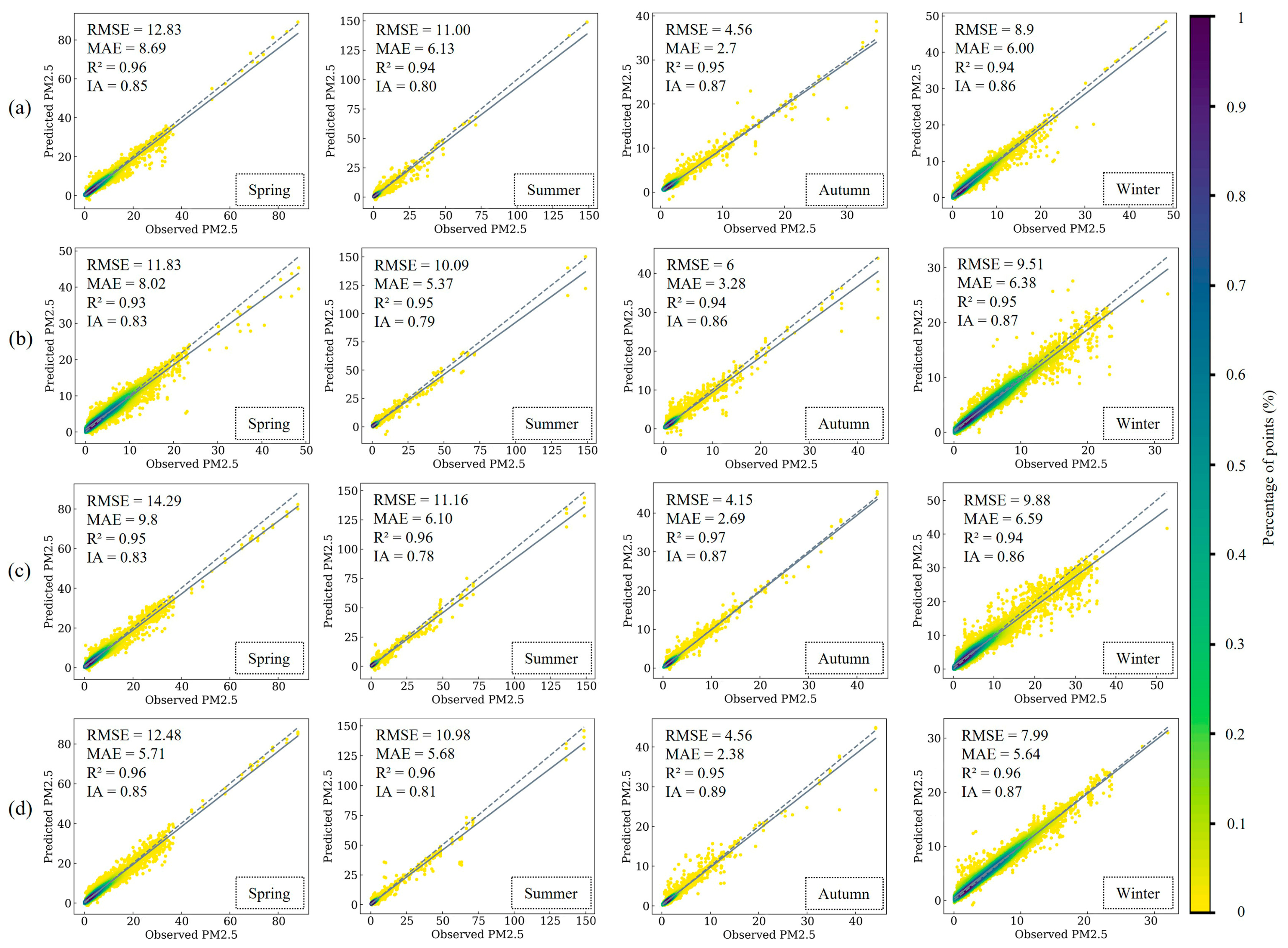
4.3.3. Seasonal Forecasting
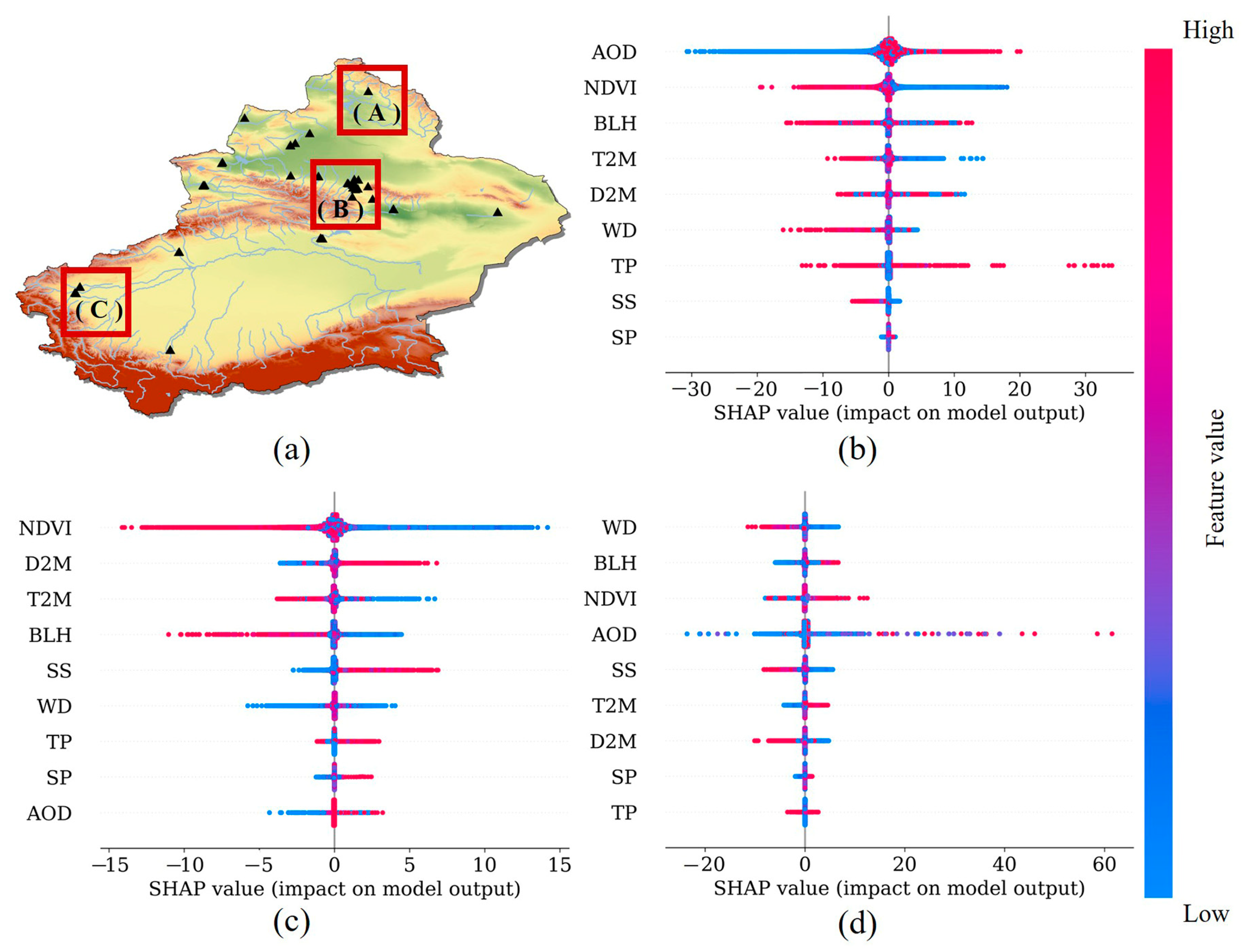
4.4. Spatiotemporal Variation of Feature Variable Based on SHAP Values
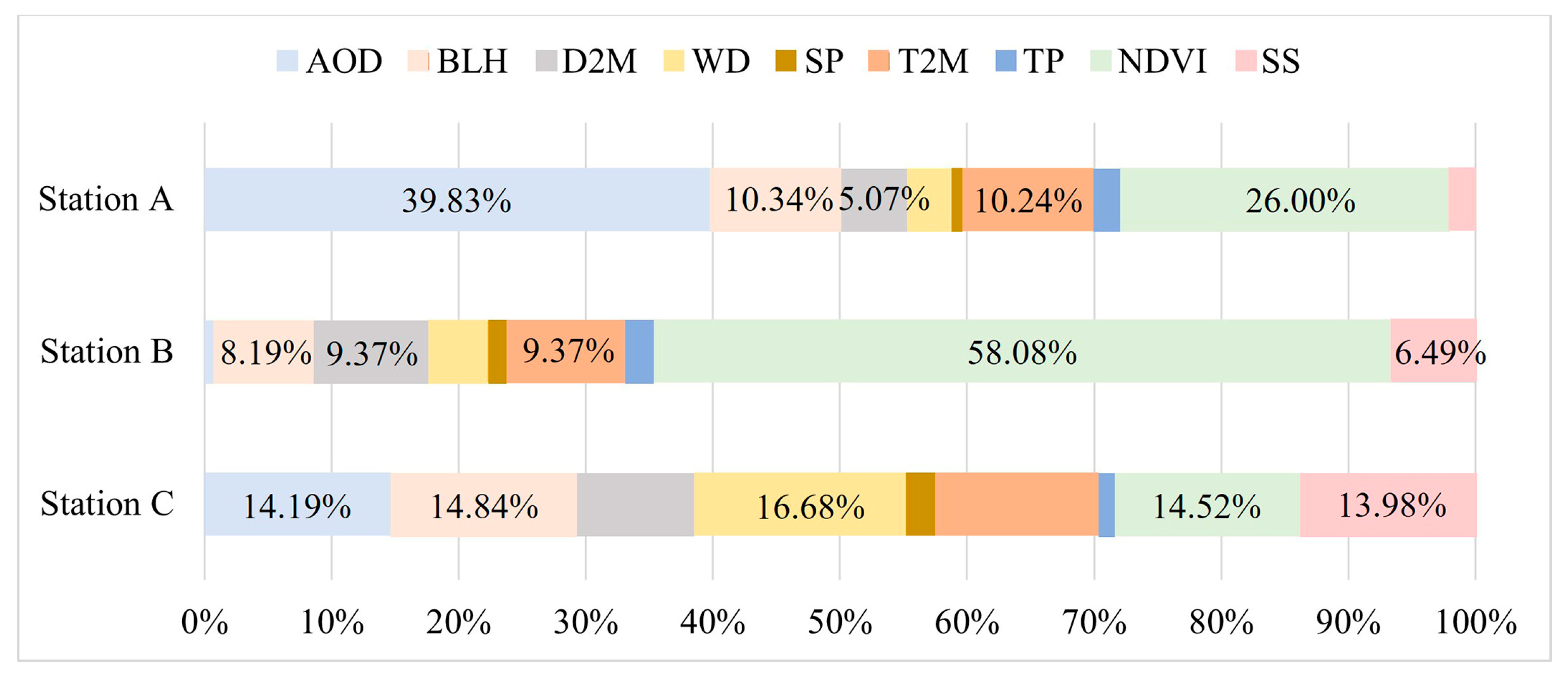
4.4.1. Overall Forecasting
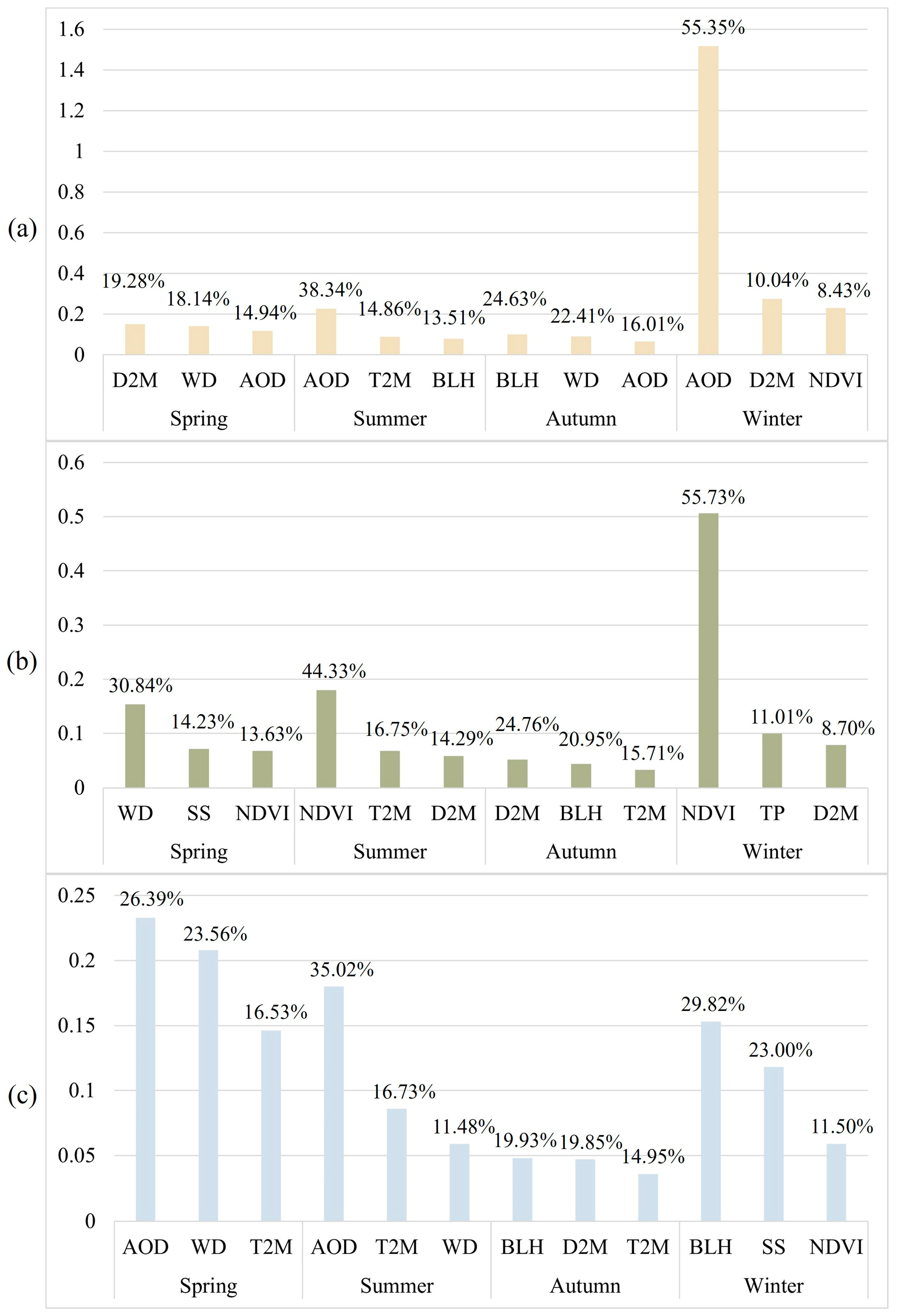
4.4.2. Seasonal Forecasting
5. Discussion
6. Conclusions
- (1)
- Temporally, PM2.5 in Xinjiang exhibits significant seasonal variations, forming a U-shaped pattern on annual and monthly scales. Spatially, the annual average concentration of PM2.5 in Xinjiang shows a trend of being higher in the southwest and lower in the northeast. The PM2.5 concentration in this region demonstrates notable spatiotemporal variations.
- (2)
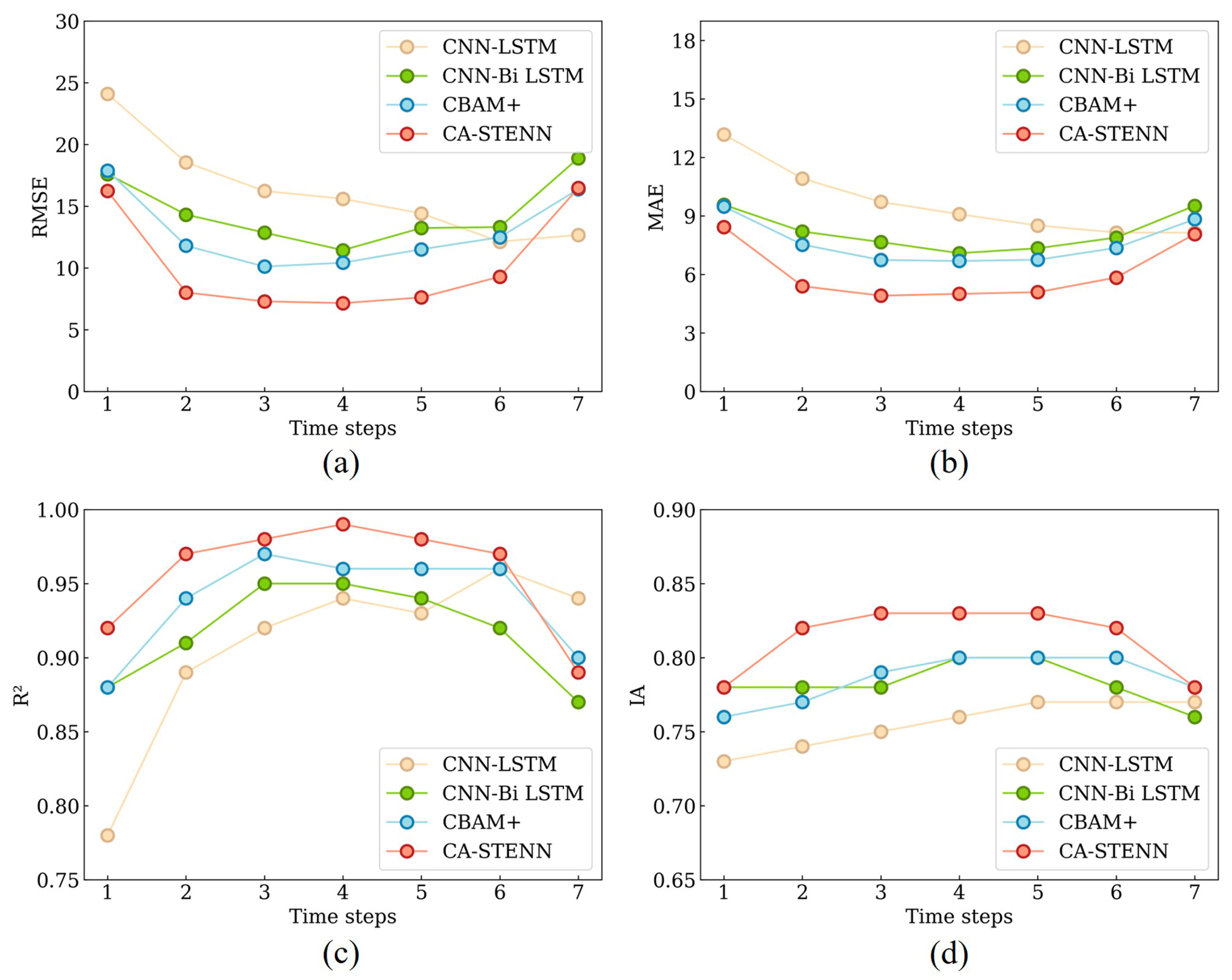
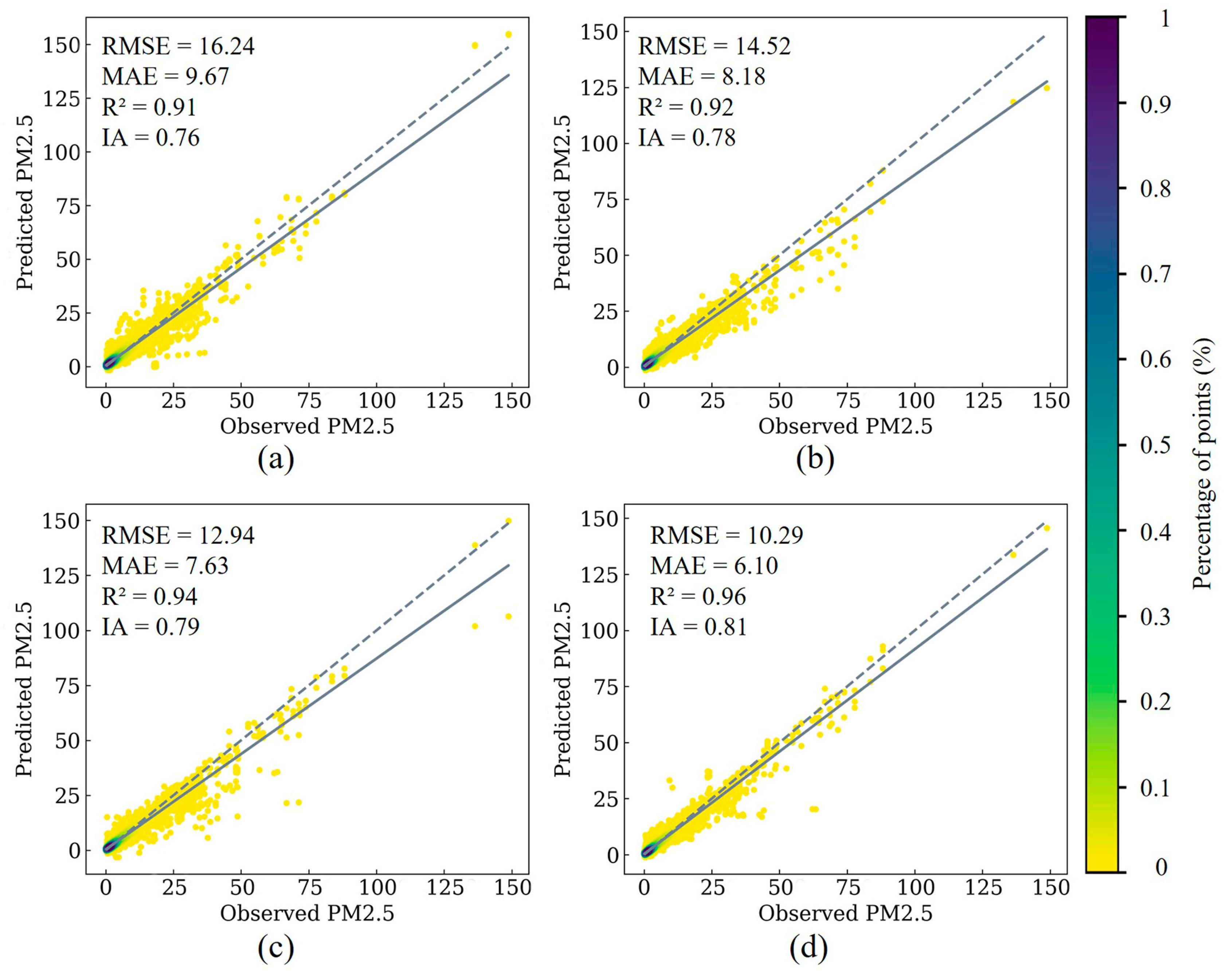
- STWNN demonstrates significantly improved predictive accuracy compared with most previous models (CNN–LSTM, CNN–Bi-LSTM, and CBAM+). Performance is relatively enhanced for seasonal predictions compared with the overall predictions. STWNN is considered the top-performing model for overall and seasonal predictions. Error pattern analysis further indicates that STWNN (0.006, p < 0.05) captures spatial heterogeneity, exhibiting strong spatiotemporal adaptability.
- (3)
- This study introduces SHAP methods for in-depth analysis of the STWNN prediction model, enhancing its interpretability and credibility. SHAP reveals the importance and spatiotemporal variation of key factors affecting PM2.5 predictions. Results indicate that AOD, BLH, and NDVI are the most influential feature variables in generating PM2.5 in Xinjiang.
Author Contributions
Funding
Institutional Review Board Statement
Informed Consent Statement
Data Availability Statement
Conflicts of Interest
References
- Chen, F.; Chen, Z. Cost of Economic Growth: Air Pollution and Health Expenditure. Sci. Total Environ. 2021, 755, 142543. [Google Scholar] [CrossRef] [PubMed]
- Li, W.; Tian, A.; Shi, Y.; Chen, B.; Ji, R.; Ge, J.; Su, X.; Pu, B.; Lei, L.; Ma, R.; et al. Associations of Long-Term Fine Particulate Matter Exposure with All-Cause and Cause-Specific Mortality: Results from the ChinaHEART Project. Lancet Reg. Health West. Pac. 2023, 41, 100908. [Google Scholar] [CrossRef] [PubMed]
- Liu, Y.; Zhou, Y.; Lu, J. Exploring the Relationship between Air Pollution and Meteorological Conditions in China under Environmental Governance. Sci. Rep. 2020, 10, 14518. [Google Scholar] [CrossRef] [PubMed]
- Foley, K.M.; Roselle, S.J.; Appel, K.W.; Bhave, P.V.; Pleim, J.E.; Otte, T.L.; Mathur, R.; Sarwar, G.; Young, J.O.; Gilliam, R.C.; et al. Incremental Testing of the Community Multiscale Air Quality (CMAQ) Modeling System Version 4.7. Geosci. Model Dev. 2010, 3, 205–226. [Google Scholar] [CrossRef]
- Tie, X.; Madronich, S.; Li, G.H.; Ying, Z.; Zhang, R.; Garcia, A.R.; Lee-Taylor, J.; Liu, Y. Characterizations of Chemical Oxidants in Mexico City: A Regional Chemical Dynamical Model (WRF-Chem) Study. Atmos. Environ. 2007, 41, 1989–2008. [Google Scholar] [CrossRef]
- Shi, L.; Zhang, H.; Xu, X.; Han, M.; Zuo, P. A Balanced Social LSTM for PM2.5 Concentration Prediction Based on Local Spatiotemporal Correlation. Chemosphere 2022, 291, 133124. [Google Scholar] [CrossRef] [PubMed]
- Yan, R.; Liao, J.; Yang, J.; Sun, W.; Nong, M.; Li, F. Multi-Hour and Multi-Site Air Quality Index Forecasting in Beijing Using CNN, LSTM, CNN-LSTM, and Spatiotemporal Clustering. Expert. Syst. Appl. 2021, 169, 114513. [Google Scholar] [CrossRef]
- Wang, J.; Wu, T.; Mao, J.; Chen, H. A Forecasting Framework on Fusion of Spatiotemporal Features for Multi-Station PM2.5. Expert. Syst. Appl. 2024, 238, 121951. [Google Scholar] [CrossRef]
- Schaap, M.; Apituley, A.; Timmermans, R.M.A.; Koelemeijer, R.B.A.; De Leeuw, G. Atmospheric Chemistry and Physics Exploring the Relation between Aerosol Optical Depth and PM 2.5 at Cabauw, the Netherlands. Atmos. Chem. Phys. 2009, 9, 909–925. [Google Scholar] [CrossRef]
- Engel-Cox, J.A.; Holloman, C.H.; Coutant, B.W.; Hoff, R.M. Qualitative and Quantitative Evaluation of MODIS Satellite Sensor Data for Regional and Urban Scale Air Quality. Atmos. Environ. 2004, 38, 2495–2509. [Google Scholar] [CrossRef]
- Xiao, Q.; Wang, Y.; Chang, H.H.; Meng, X.; Geng, G.; Lyapustin, A.; Liu, Y. Full-Coverage High-Resolution Daily PM2.5 Estimation Using MAIAC AOD in the Yangtze River Delta of China. Remote Sens. Environ. 2017, 199, 437–446. [Google Scholar] [CrossRef]
- Zhang, T.; Zhu, Z.; Gong, W.; Zhu, Z.; Sun, K.; Wang, L.; Huang, Y.; Mao, F.; Shen, H.; Li, Z.; et al. Estimation of Ultrahigh Resolution PM2.5 Concentrations in Urban Areas Using 160 m Gaofen-1 AOD Retrievals. Remote Sens. Environ. 2018, 216, 91–104. [Google Scholar] [CrossRef]
- Feng, L.; Wang, Y.; Zhang, Z.; Du, Q. Geographically and Temporally Weighted Neural Network for Winter Wheat Yield Prediction. Remote Sens. Environ. 2021, 262, 112514. [Google Scholar] [CrossRef]
- O’SULLIVAN, D. Geographically Weighted Regression: The Analysis of Spatially Varying Relationships, by A. S. Fotheringham, C. Brunsdon, and M. Charlton. Geogr. Anal. 2003, 35, 272–275. [Google Scholar] [CrossRef]
- Dai, Z.; Wu, S.; Wang, Y.; Zhou, H.; Zhang, F.; Huang, B.; Du, Z. Geographically Convolutional Neural Network Weighted Regression: A Method for Modeling Spatially Non-Stationary Relationships Based on a Global Spatial Proximity Grid. Int. J. Geogr. Inf. Sci. 2022, 36, 2248–2269. [Google Scholar] [CrossRef]
- Hu, X.; Waller, L.A.; Lyapustin, A.; Wang, Y.; Al-Hamdan, M.Z.; Crosson, W.L.; Estes, M.G.; Estes, S.M.; Quattrochi, D.A.; Puttaswamy, S.J.; et al. Estimating Ground-Level PM2.5 Concentrations in the Southeastern United States Using MAIAC AOD Retrievals and a Two-Stage Model. Remote Sens. Environ. 2014, 140, 220–232. [Google Scholar] [CrossRef]
- Li, R.; Gong, J.; Chen, L.; Wang, Z. Estimating Ground-Level PM2.5 Using Fine-Resolution Satellite Data in the Megacity of Beijing, China. Aerosol Air Qual. Res. 2015, 15, 1347–1356. [Google Scholar] [CrossRef]
- Wu, J.; Yao, F.; Li, W.; Si, M. VIIRS-Based Remote Sensing Estimation of Ground-Level PM2.5 Concentrations in Beijing–Tianjin–Hebei: A Spatiotemporal Statistical Model. Remote Sens. Environ. 2016, 184, 316–328. [Google Scholar] [CrossRef]
- Hu, X.; Waller, L.A.; Lyapustin, A.; Wang, Y.; Liu, Y. 10-Year Spatial and Temporal Trends of PM2.5 Concentrations in the Southeastern US Estimated Using High-Resolution Satellite Data. Atmos. Chem. Phys. 2014, 14, 6301–6314. [Google Scholar] [CrossRef]
- He, Q.; Huang, B. Satellite-Based Mapping of Daily High-Resolution Ground PM2.5 in China via Space-Time Regression Modeling. Remote Sens. Environ. 2018, 206, 72–83. [Google Scholar] [CrossRef]
- Fotheringham, A.S.; Crespo, R.; Yao, J. Geographical and Temporal Weighted Regression (GTWR). Geogr. Anal. 2015, 47, 431–452. [Google Scholar] [CrossRef]
- Zhao, Z.; Xu, Z.; Hu, C.; Wang, K.; Ding, X. Geographically Weighted Neural Network Considering Spatial Heterogeneity for Landslide Susceptibility Mapping: A Case Study of Yichang City, China. Catena 2024, 234, 107590. [Google Scholar] [CrossRef]
- Liu, J.; Weng, F.; Li, Z. Satellite-Based PM2.5 Estimation Directly from Reflectance at the Top of the Atmosphere Using a Machine Learning Algorithm. Atmos. Environ. 2019, 208, 113–122. [Google Scholar] [CrossRef]
- Stafoggia, M.; Bellander, T.; Bucci, S.; Davoli, M.; de Hoogh, K.; de’ Donato, F.; Gariazzo, C.; Lyapustin, A.; Michelozzi, P.; Renzi, M.; et al. Estimation of Daily PM10 and PM2.5 Concentrations in Italy, 2013–2015, Using a Spatiotemporal Land-Use Random-Forest Model. Environ. Int. 2019, 124, 170–179. [Google Scholar] [CrossRef] [PubMed]
- Wu, Y.; Guo, J.; Zhang, X.; Tian, X.; Zhang, J.; Wang, Y.; Duan, J.; Li, X. Synergy of Satellite and Ground Based Observations in Estimation of Particulate Matter in Eastern China. Sci. Total Environ. 2012, 433, 20–30. [Google Scholar] [CrossRef] [PubMed]
- Li, T.; Shen, H.; Zeng, C.; Yuan, Q.; Zhang, L. Point-Surface Fusion of Station Measurements and Satellite Observations for Mapping PM2.5 Distribution in China: Methods and Assessment. Atmos. Environ. 2017, 152, 477–489. [Google Scholar] [CrossRef]
- Wang, Z.; Hu, B.; Huang, B.; Ma, Z.; Biswas, A.; Jiang, Y.; Shi, Z. Predicting Annual PM2.5 in Mainland China from 2014 to 2020 Using Multi Temporal Satellite Product: An Improved Deep Learning Approach with Spatial Generalization Ability. ISPRS J. Photogramm. Remote Sens. 2022, 187, 141–158. [Google Scholar] [CrossRef]
- Yang, J.; Yan, R.; Nong, M.; Liao, J.; Li, F.; Sun, W. PM2.5 Concentrations Forecasting in Beijing through Deep Learning with Different Inputs, Model Structures and Forecast Time. Atmos. Pollut. Res. 2021, 12, 101168. [Google Scholar] [CrossRef]
- Yang, Q.; Yuan, Q.; Yue, L.; Li, T.; Shen, H.; Zhang, L. Mapping PM2.5 Concentration at a Sub-Km Level Resolution: A Dual-Scale Retrieval Approach. ISPRS J. Photogramm. Remote Sens. 2020, 165, 140–151. [Google Scholar] [CrossRef]
- Wang, W.; Mao, W.; Tong, X.; Xu, G. A Novel Recursive Model Based on a Convolutional Long Short-Term Memory Neural Network for Air Pollution Prediction. Remote Sens. 2021, 13, 1284. [Google Scholar] [CrossRef]
- Li, X.; Peng, L.; Yao, X.; Cui, S.; Hu, Y.; You, C.; Chi, T. Long Short-Term Memory Neural Network for Air Pollutant Concentration Predictions: Method Development and Evaluation. Environ. Pollut. 2017, 231, 997–1004. [Google Scholar] [CrossRef] [PubMed]
- Wang, Z.; Zhou, Y.; Zhao, R.; Wang, N.; Biswas, A.; Shi, Z. High-Resolution Prediction of the Spatial Distribution of PM2.5 Concentrations in China Using a Long Short-Term Memory Model. J. Clean. Prod. 2021, 297, 126493. [Google Scholar] [CrossRef]
- Woo, S.; Park, J.; Lee, J.-Y.; Kweon, I.S. CBAM: Convolutional Block Attention Module; Springer: Cham, Switzerland, 2018. [Google Scholar]
- Li, D.; Liu, J.; Zhao, Y. Prediction of Multi-Site PM2.5 Concentrations in Beijing Using CNN-Bi LSTM with CBAM. Atmosphere 2022, 13, 1719. [Google Scholar] [CrossRef]
- Huang, C.J.; Kuo, P.H. A Deep Cnn-Lstm Model for Particulate Matter (PM2.5) Forecasting in Smart Cities. Sensors 2018, 18, 2220. [Google Scholar] [CrossRef] [PubMed]
- Su, Y.; Li, J.; Liu, L.; Guo, X.; Huang, L.; Hu, M. Application of CNN-LSTM Algorithm for PM2.5 Concentration Forecasting in the Beijing-Tianjin-Hebei Metropolitan Area. Atmosphere 2023, 14, 1392. [Google Scholar] [CrossRef]
- Ding, C.; Wang, G.; Zhang, X.; Liu, Q.; Liu, X. A Hybrid CNN-LSTM Model for Predicting PM2.5 in Beijing Based on Spatiotemporal Correlation. Environ. Ecol. Stat. 2021, 28, 503–522. [Google Scholar] [CrossRef]
- Wang, Z.; Li, R.; Chen, Z.; Yao, Q.; Gao, B.; Xu, M.; Yang, L.; Li, M.; Zhou, C. The Estimation of Hourly PM2.5 Concentrations across China Based on a Spatial and Temporal Weighted Continuous Deep Neural Network (STWC-DNN). ISPRS J. Photogramm. Remote Sens. 2022, 190, 38–55. [Google Scholar] [CrossRef]
- Li, T.; Shen, H.; Yuan, Q.; Zhang, L. A Locally Weighted Neural Network Constrained by Global Training for Remote Sensing Estimation of PM. IEEE Trans. Geosci. Remote Sens. 2022, 60, 1–13. [Google Scholar] [CrossRef]
- Xue, Y.; Li, Y.; Guang, J.; Tugui, A.; She, L.; Qin, K.; Fan, C.; Che, Y.; Xie, Y.; Wen, Y.; et al. Hourly PM2.5 Estimation over Central and Eastern China Based on Himawari-8 Data. Remote Sens. 2020, 12, 855. [Google Scholar] [CrossRef]
- Qi, Y.; Li, Q.; Karimian, H.; Liu, D. A Hybrid Model for Spatiotemporal Forecasting of PM 2.5 Based on Graph Convolutional Neural Network and Long Short-Term Memory. Sci. Total Environ. 2019, 664, 1–10. [Google Scholar] [CrossRef]
- Li, T.; Zhang, C.; Shen, H.; Yuan, Q.; Zhang, L. Real-Time and Seamless Monitoring of Ground-Level Pm2.5 Using Satellite Remote Sensing. arXiv 2018, arXiv:1803.03409. [Google Scholar] [CrossRef]
- Quan, W.; Xia, N.; Guo, Y.; Hai, W.; Song, J.; Zhang, B. PM2.5 Concentration Assessment Based on Geographical and Temporal Weighted Regression Model and MCD19A2 from 2015 to 2020 in Xinjiang, China. PLoS ONE 2023, 18, e0285610. [Google Scholar] [CrossRef] [PubMed]
- Jin, X.Y.; Ding, J.; Ge, X.; Liu, J.; Xie, B.; Zhao, S.; Zhao, Q. Machine Learning Driven by Environmental Covariates to Estimate High-Resolution PM2.5 in Data-Poor Regions. PeerJ 2022, 10, e13203. [Google Scholar] [CrossRef] [PubMed]
- Ren, M.; Sun, W.; Chen, S. Combining Machine Learning Models through Multiple Data Division Methods for PM2.5 Forecasting in Northern Xinjiang, China. Environ. Monit. Assess. 2021, 193, 476. [Google Scholar] [CrossRef] [PubMed]
- Wang, Y.; Zhang, J.; Bai, Z.; Yang, W.; Zhang, H.; Mao, J.; Sun, Y.L.; Ma, Z.; Xiao, J.; Gao, S.; et al. Background Concentrations of PMs in Xinjiang, West China: An Estimation Based on Meteorological Filter Method and Eckhardt Algorithm. Atmos. Res. 2019, 215, 141–148. [Google Scholar] [CrossRef]
- Wang, J.; Christopher, S.A. Intercomparison between Satellite-Derived Aerosol Optical Thickness and PM2.5 Mass: Implications for Air Quality Studies. Geophys. Res. Lett. 2003, 30, 2095. [Google Scholar] [CrossRef]
- Li, R.; Mei, X.; Chen, L.; Wang, Z.; Jing, Y.; Wei, L. Influence of Spatial Resolution and Retrieval Frequency on Applicability of Satellite-Predicted Pm2.5 in Northern China. Remote Sens. 2020, 12, 736. [Google Scholar] [CrossRef]
- Chen, Z.; Chen, D.; Zhao, C.; Kwan, M.-P.; Cai, J.; Zhuang, Y.; Zhao, B.; Wang, X.; Chen, B.; Yang, J.; et al. Influence of Meteorological Conditions on PM2.5 Concentrations across China: A Review of Methodology and Mechanism. Environ. Int. 2020, 139, 105558. [Google Scholar] [CrossRef] [PubMed]
- Liu, Y.; Paciorek, C.J.; Koutrakis, P. Estimating Regional Spatial and Temporal Variability of PM2.5 Concentrations Using Satellite Data, Meteorology, and Land Use Information. Environ. Health Perspect. 2009, 117, 886–892. [Google Scholar] [CrossRef] [PubMed]
- Lu, D.; Mao, W.; Yang, D.; Zhao, J.; Xu, J. Effects of Land-Use and Landscape Pattern on PM2.5 in Yangtze River Delta in China. Atmos. Pollut. Res. 2018, 9, 705–713. [Google Scholar] [CrossRef]
- Claridge, D.E.; Chen, H. Missing Data Estimation for 1–6 h Gaps in Energy Use and Weather Data Using Different Statistical Methods. Int. J. Energy Res. 2006, 30, 1075–1091. [Google Scholar] [CrossRef]
- Moran, P.A.P. Notes on Continuous Stochastic Phenomena; Oxford University Press: Oxford, UK, 2014; Volume 11. [Google Scholar]
- Anselin, L. Local Indicators of Spatial Association—LISA. Geogr. Anal. 1995, 27, 93–115. [Google Scholar] [CrossRef]
- Li, T.; Shen, H.; Yuan, Q.; Zhang, X.; Zhang, L. Estimating Ground-Level PM2.5 by Fusing Satellite and Station Observations: A Geo-Intelligent Deep Learning Approach. Geophys. Res. Lett. 2017, 44, 11985–11993. [Google Scholar] [CrossRef]
- Xue, T.; Zheng, Y.; Tong, D.; Zheng, B.; Li, X.; Zhu, T.; Zhang, Q. Spatiotemporal Continuous Estimates of PM2.5 Concentrations in China, 2000–2016: A Machine Learning Method with Inputs from Satellites, Chemical Transport Model, and Ground Observations. Environ. Int. 2019, 123, 345–357. [Google Scholar] [CrossRef] [PubMed]
- Zhou, P.; Shi, W.; Tian, J.; Qi, Z.; Li, B.; Hao, H.; Xu, B. Attention-Based Bidirectional Long Short-Term Memory Networks for Relation Classification; Association for Computational Linguistics: New Brunswick, NJ, USA, 2016. [Google Scholar]
- Qin, D.; Yu, J.; Zou, G.; Yong, R.; Zhao, Q.; Zhang, B. A Novel Combined Prediction Scheme Based on CNN and LSTM for Urban PM2.5 Concentration. IEEE Access 2019, 7, 20050–20059. [Google Scholar] [CrossRef]
- Lundberg, S.M.; Allen, P.G.; Lee, S.-I. A Unified Approach to Interpreting Model Predictions. In Proceedings of the Advances in Neural Information Processing Systems 30 (NIPS 2017), Long Beach, CA, USA, 4–9 December 2017. [Google Scholar]
- Yang, Y.; Mei, G.; Izzo, S. Revealing Influence of Meteorological Conditions on Air Quality Prediction Using Explainable Deep Learning. IEEE Access 2022, 10, 50755–50773. [Google Scholar] [CrossRef]
- Boulesteix, A.L.; Bender, A.; Bermejo, J.L.; Strobl, C. Random Forest Gini Importance Favours SNPs with Large Minor Allele Frequency: Impact, Sources and Recommendations. Brief. Bioinform. 2012, 13, 292–304. [Google Scholar] [CrossRef]
- Wei, J.; Li, Z.; Lyapustin, A.; Sun, L.; Peng, Y.; Xue, W.; Su, T.; Cribb, M. Reconstructing 1-Km-Resolution High-Quality PM2.5 Data Records from 2000 to 2018 in China: Spatiotemporal Variations and Policy Implications. Remote Sens. Environ. 2021, 252, 112136. [Google Scholar] [CrossRef]
- Chen, S.; Tong, B.; Russell, L.M.; Wei, J.; Guo, J.; Mao, F.; Liu, D.; Huang, Z.; Xie, Y.; Qi, B.; et al. Lidar-Based Daytime Boundary Layer Height Variation and Impact on the Regional Satellite-Based PM2.5 Estimate. Remote Sens. Environ. 2022, 281, 113224. [Google Scholar] [CrossRef]
- Zheng, B.; Zhang, Q.; Zhang, Y.; He, K.B.; Wang, K.; Zheng, G.J.; Duan, F.K.; Ma, Y.L.; Kimoto, T. Heterogeneous Chemistry: A Mechanism Missing in Current Models to Explain Secondary Inorganic Aerosol Formation during the January 2013 Haze Episode in North China. Atmos. Chem. Phys. 2015, 15, 2031–2049. [Google Scholar] [CrossRef]
- Wang, J.; Ogawa, S. Effects of Meteorological Conditions on PM2.5 Concentrations in Nagasaki, Japan. Int. J. Environ. Res. Public. Health 2015, 12, 9089–9101. [Google Scholar] [CrossRef]
- Gao, S.; Cheng, X.; Yu, J.; Chen, L.; Sun, Y.; Bai, Z.; Xu, H.; Azzi, M.; Zhao, H. Meteorological Influences on PM2.5 Variation in China Using a Hybrid Model of Machine Learning and the Kolmogorov-Zurbenko Filter. Atmos. Pollut. Res. 2023, 14, 101905. [Google Scholar] [CrossRef]


| Type | Variable | Unit | Spatial Resolution | Temporal Resolution |
|---|---|---|---|---|
| Pollutant | PM2.5 | ug/m3 | Station | 1 h |
| Optical | AOD | N/A | 1 km | 1 day |
| Meteorology | BLH | m | 0.25° | 1 h |
| D2M | k | 0.25° | 1 h | |
| WD | m/s | 0.25° | 1 h | |
| SP | pa | 0.25° | 1 h | |
| T2M | k | 0.25° | 1 h | |
| TP | m | 0.25° | 1 h | |
| Land-related | NDVI | N/A | 1 km | 16 days |
| Longitude | ° | N/A | N/A | |
| Latitude | ° | N/A | N/A |
| Parameters | Value |
|---|---|
| N (SS) | 3 |
| Kernel size of CNN | 4 × 4 |
| Convolution channels | 32 |
| Convolution layer | 3 |
| Channel convolution kernel size | 3 × 3 |
| Bi-LSTM nodes | 256, 128 |
| Bi-LSTM layer | 2 |
| Fully connected layer nodes | 46 |
| Learning rate | Adam |
| Batch size | 8 |
| Epochs | 1000 |
| n | RMSE | MAE | R2 | IA |
|---|---|---|---|---|
| 1 | 13.23 | 7.79 | 0.94 | 0.79 |
| 2 | 13.24 | 7.66 | 0.93 | 0.79 |
| 3 | 10.29 | 6.1 | 0.96 | 0.81 |
| 4 | 13.26 | 7.9 | 0.94 | 0.78 |
| 5 | 12.89 | 7.08 | 0.94 | 0.79 |
| STWNN | RMSE | MAE | R2 | IA |
|---|---|---|---|---|
| Overall | 10.29 | 6.10 | 0.96 | 0.81 |
| Spring | 12.48 | 5.71 | 0.96 | 0.85 |
| Summer | 10.99 | 5.68 | 0.96 | 0.81 |
| Autumnn | 4.56 | 2.38 | 0.95 | 0.89 |
| Winter | 7.99 | 5.64 | 0.96 | 0.87 |
Disclaimer/Publisher’s Note: The statements, opinions and data contained in all publications are solely those of the individual author(s) and contributor(s) and not of MDPI and/or the editor(s). MDPI and/or the editor(s) disclaim responsibility for any injury to people or property resulting from any ideas, methods, instructions or products referred to in the content. |
© 2024 by the authors. Licensee MDPI, Basel, Switzerland. This article is an open access article distributed under the terms and conditions of the Creative Commons Attribution (CC BY) license (https://creativecommons.org/licenses/by/4.0/).
Share and Cite
Wu, Y.; Xu, Z.; Xu, L.; Wei, J. An Improved Deep Learning Approach Considering Spatiotemporal Heterogeneity for PM2.5 Prediction: A Case Study of Xinjiang, China. Atmosphere 2024, 15, 460. https://doi.org/10.3390/atmos15040460
Wu Y, Xu Z, Xu L, Wei J. An Improved Deep Learning Approach Considering Spatiotemporal Heterogeneity for PM2.5 Prediction: A Case Study of Xinjiang, China. Atmosphere. 2024; 15(4):460. https://doi.org/10.3390/atmos15040460
Chicago/Turabian StyleWu, Yajing, Zhangyan Xu, Liping Xu, and Jianxin Wei. 2024. "An Improved Deep Learning Approach Considering Spatiotemporal Heterogeneity for PM2.5 Prediction: A Case Study of Xinjiang, China" Atmosphere 15, no. 4: 460. https://doi.org/10.3390/atmos15040460
APA StyleWu, Y., Xu, Z., Xu, L., & Wei, J. (2024). An Improved Deep Learning Approach Considering Spatiotemporal Heterogeneity for PM2.5 Prediction: A Case Study of Xinjiang, China. Atmosphere, 15(4), 460. https://doi.org/10.3390/atmos15040460