Assessing the Potential for Photochemical Reflectance Index to Improve the Relationship between Solar-Induced Chlorophyll Fluorescence and Gross Primary Productivity in Crop and Soybean

Abstract

Photosynthesis is influenced by dynamic energy allocation under various environmental conditions. Solar-induced chlorophyll fluorescence (SIF), an important pathway for dissipating absorbed energy, has been extensively used to evaluate gross primary productivity (GPP). However, the potential for photochemical reflectance index (PRI), as an indicator of non-photochemical quenching (NPQ), to improve the SIF-based GPP estimation, has not been thoroughly investigated. In this study, using continually tower-based observations, we examined how PRI affected the link between SIF and GPP for corn and soybean at half-hourly and daily timescales. The relationship of GPP to SIF and PRI is impacted by stress indicated by vapor pressure deficit (VPD) and crop water stress index (CWSI). Moreover, the ratio of GPP to SIF of corn was more sensitive to PRI compared to soybean. Whether in Pearson or Partial correlation analysis, the relationships of PRI to the ratio of GPP to SIF were almost all significant, regardless of controlling structural-physiological (stomatal conductance, vegetation indices) and environmental variables (light intensity, etc.). Therefore, PRI significantly affects the SIF–GPP relationship for corn (r > 0.31, p < 0.01) and soybean (r > 0.22, p < 0.05). After combining SIF and PRI using the multi-variable linear model, the GPP estimation has been largely improved (the coefficient of determination, abbreviated as R², increased from 0.48 to 0.49 to 0.78 to 0.84 and the Root Mean Square Error, abbreviated as RMSE, decreased from 6.38 to 10.22 to 3.56 to 6.60 $\mathsf{\mu }\mathrm{m}\mathrm{o}\mathrm{l} {\mathrm{C}\mathrm{O}}_2·{\mathrm{m}}^{-2}·{\mathrm{s}}^{-1}$ for corn, R² increased from 0.54 to 0.62 to 0.78 to 0.82 and RMSE decreased from 6.25 to 9.59 to 4.34 to 6.60 $\mathsf{\mu }\mathrm{m}\mathrm{o}\mathrm{l} {\mathrm{C}\mathrm{O}}_2·{\mathrm{m}}^{-2}·{\mathrm{s}}^{-1}$ for soybean). It suggests that better GPP estimations for corn and soybean can be obtained when SIF is combined with PRI.

1. Introduction

Plant gross primary productivity (GPP) is the largest terrestrial carbon flux in the carbon cycle and is essential for regulating climatic and environmental changes on Earth [1,2]. To estimate GPP at in situ or regional scales, the vegetation indices, the physically processed model, and the light-use efficiency model have been suggested [3]. However, the drawbacks of using a lot of computing power and the absence of description of different photosynthetic processes limit the instantaneous accuracy of GPP estimation and make it challenging to track the dynamic variations of GPP in response to environmental changes.

It has been established that an energy dissipated pathway known as solar-induced chlorophyll fluorescence (SIF), which is directly related to the light reactions, is a superior way to monitor GPP dynamics, particularly under stressful conditions [4]. The chlorophyll molecules get excited as a result of absorbing photosynthetically active radiation (APAR). Three processes—photochemical quenching (PQ), non-radiative decay or non-photochemical quenching (NPQ), and fluorescence—can be used to dissipate the excitation energy [5]. The three energy-dissipating pathways compete with one another and display various patterns in response to the constantly changing external environment. SIF and GPP have an inherent theoretical foundation for coupling since APAR drives both SIF and GPP. In reality, the mechanism for using SIF to predict GPP is the link between the linear electron transfer rate (ETR) coupled with carboxylation processes and SIF [6]. According to the light-use-efficiency framework, GPP is computed as the product of APAR and light use efficiency (${LUE}_p$), which is expressed as follows:

$$GPP=APAR\times {LUE}_p$$

(1)

Likewise, canopy observed SIF at a certain direction (${SIF}_c$) can be represented as the product of APAR and the apparent yield for fluorescence, which consists of the escaping probability ($f_{esc}$) at the same direction and the photosystem fluorescence yield (${\Phi }_f$):

$${SIF}_c=APAR\times {\Phi }_f\times f_{esc}$$

(2)

Due to the complex horizontal and vertical structures of the canopy, the emitted SIF by leaves would experience the scattering of the reabsorption effects before sensors capture [7,8]. Additionally, because of the limited field of view (FOV) of the sensors, the hemispherical SIF emission can only be captured in the observation direction. Based on a multi-angle observational experiment, Liu et al. [9] revealed that SIF and reflectance have an angle effect that is similar. Numerous studies have shown that using the spectral invariant theory, the escaping probability of SIF at one angle can be approximately estimated by the canopy measured reflectance at the same angle divided by the product of its interception and leaf albedo [10,11,12,13]. To obtain the total SIF (${SIF}_t$) with more physiological information, the impacts of observed angle and canopy structure should be eliminated:

$${SIF}_t=\frac{{SIF}_c}{f_{esc}}$$

(3)

As a result, the relationship between ${LUE}_p$ and ${\Phi }_f$ is the primary factor for linking GPP to SIF. However, the aforementioned LUE framework for linking SIF to GPP has clear disadvantages in describing various photosynthetic processes because it simplifies the photosynthetic process, including the light and dark reactions, which may differ in response to environmental stress [6].

Environmental variables such as air temperature, soil moisture, and light intensity have an influence on the SIF–GPP relationship. Despite the fact that APAR drives both SIF and GPP, some studies found there was a stronger relationship of APAR to SIF than that of APAR to GPP, and the ratio of GPP to SIF decreased with light intensity. These findings may be related to the differences between light and dark reactions or the irregularly varied proportion of energy allocated to SIF and photosynthesis [14]. Despite the fact that SIF can monitor the downregulation of GPP in response to drought conditions at both leaf and canopy levels, water deficit also affects the link of SIF to GPP [15]. Likewise, the SIF–GPP relationship is also somewhat impacted by the photochemistry activities and the kinetics of enzymes involved in carbon reactions, which are both affected by temperature [16]. The SIF–GPP relationship can be altered by the dynamic energy distribution among three energy dissipation pathways in response to various temperature conditions. Additionally, the SIF–GPP relationship depends heavily on the chlorophyll content, which could explain why SIF and GPP have different growth peaks [17]. Plants with the two distinct photosynthetic pathways, C3 and C4, are typically regarded as two major plant functional types (PFT) in climate-carbon models because of their significant differences in environmental requirements and global change feedback. C4 plants have higher resource-use efficiency and potential productivity because they have evolved from the C4 route to adapt to high light intensity, high temperature, and dryness through C4 photosynthesis. In C4 species, the effect of diffusional pathways on the SIF–GPP relationship is mitigated by the cooperation of mesophyll and bundle sheath cells to concentrate CO₂ near Rubisco. The fact that distinct PFTs have different metabolic pathways may explain why there are differences in the slopes between SIF and GPP for these PFTs [9].

SIF, a single energy dissipation pathway, is insufficient to effectively account for the dynamic fluctuations in GPP under stress. As one of three pathways for consuming the solar energy absorbed by leaves, NPQ may thus play a controlled role in the distribution of energy between fluorescence and PQ [18]. The downregulation of photosynthetic efficiency at diurnal timescales is often correlated with the degree of epoxidation in the xanthophyll pigments, which increases under stress in leaves [19]. Under stress, xanthophyll de-epoxidation typically causes a rise in NPQ. Some investigations have discovered that the photochemical reflectance index (PRI), which often exhibits a negative connection with NPQ, might describe the epoxidation status of xanthophyll pigments [20]. Variations in PRI can well represent changes in NPQ generated by the xanthophyll cycle in response to the external environment because of sluggish adjustments in pigment pools at diurnal timescales. However, at seasonal timescales, the changes in the carotenoid and chlorophyll pigment pools in leaves can also contribute to the differences in PRI [21,22]. Therefore, at a specific chlorophyll content level, PRI can be utilized to characterize NPQ fluctuations at an instantaneous or daily scale, and it is important to thoroughly investigate the potential effects of PRI variation on the SIF–GPP relationship.

Under the premise of some aspects of the information regarding NPQ that can be estimated from PRI, it makes sense to study the influences of PRI on the SIF-based GPP estimation. Wang et al. [18] used MODIS PRI, OCO-2 SIF observations, and contemporaneous flux data from EC locations to evaluate the value of PRI for the SIF-based GPP estimation. However, because of various data sources and broad spatial scales, the conclusions are highly unclear. Recently, a large amount of continuously tower-based observations can offer us trustworthy data to study the SIF–GPP relationship and its reaction to various environmental conditions [2,19,23]. To measure radiance from a downwelling and upwelling direction, a number of tower-based spectral systems with a bi-hemispherical or hemispherical-conical setup have been developed. According to Miao et al. [24], some spectral systems (e.g., FluoSpec2) contain two subsystems, one for SIF retrieval and the other for calculating vegetation indices (VI), such as the normalized difference vegetation index (NDVI), PRI. Therefore, we may explore the potential influences of PRI on the SIF–GPP relationship at diurnal and seasonal scales using the continuous observations. In addition, the information from reflectance-based PRI and SIF can be used to estimate GPP at global scales in the future thanks to the launch of the European Space Agency’s (ESA) Fluorescence Explorer (FLEX) mission [11,25]. Although the fact that the combination of SIF, PRI, and structure information has been proven to be beneficial for quantifying GPP based on airborne or satellite observations, the potential impact of PRI on the relationship of GPP to SIF for C3 and C4 crops has yet to be investigated based on tower-based measurements.

According to the key hypotheses and the theoretical foundation proposed by Wang et al. [18], the usefulness of combining the information of NPQ reflected by PRI with ${SIF}_t$ to improve GPP estimation was examined for soybean (a C3 crop) and corn (a C4 crop) crops based on tower-based measurements in this study. The specific issues to be addressed in detail including: (1) How might PRI affect the ${SIF}_t$–GPP relationships? (2) How might these relationships differ for C3 (soybean) and C4 (corn) crops? (3) Is it possible to increase the accuracy of the GPP estimation by combining PRI and ${SIF}_t$?

2. Materials and Methods

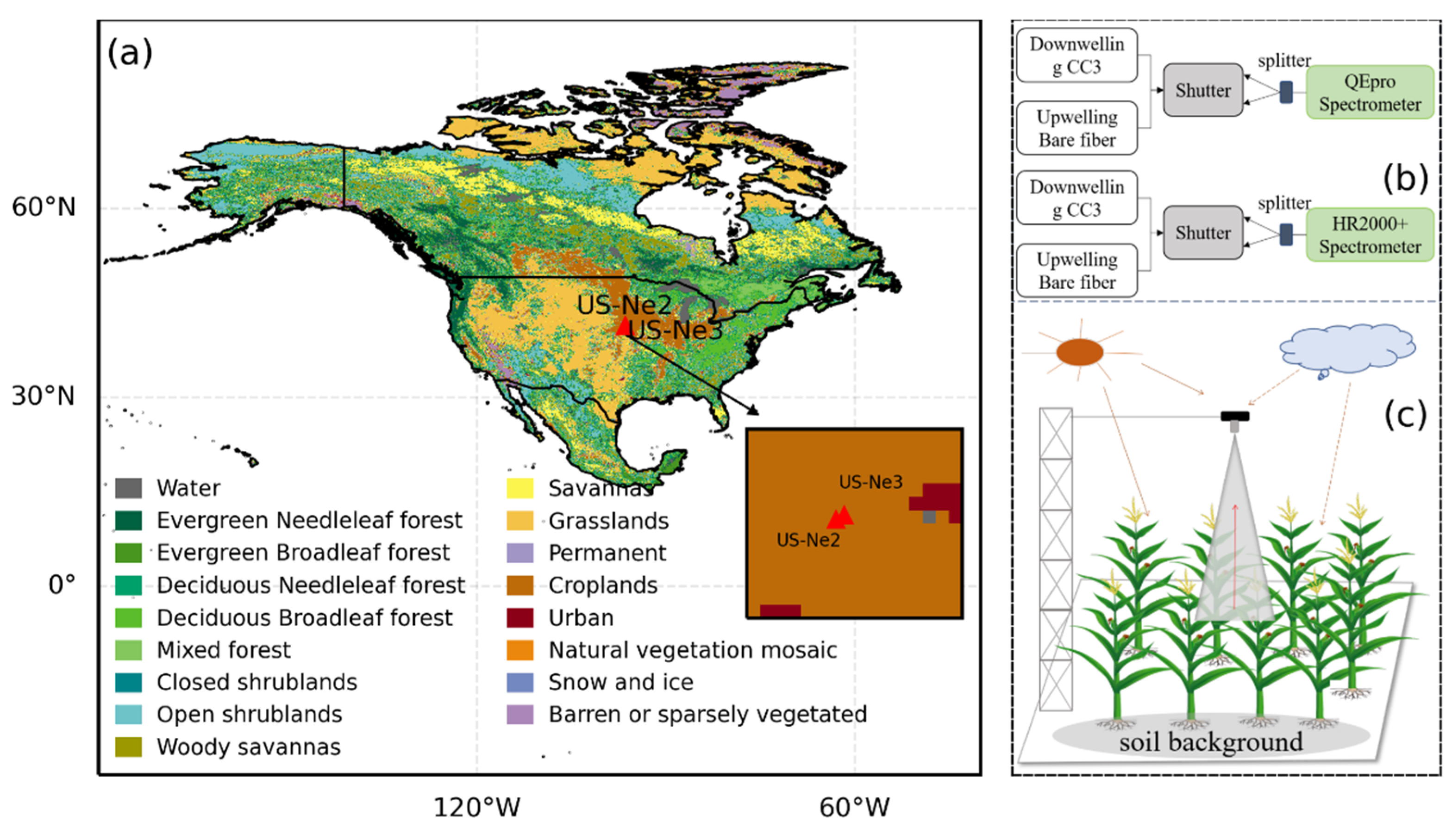
2.1. Site Description

This study used an open-access dataset, which was collected at the US-Ne2 (41.1649° N, 96.4701° W) and US-Ne3 (41.1797° N, 96.4397° W) sites in Lincoln, NE, USA [26]. Two FluoSpec2 systems were installed near planting and uninstalled after the harvest in order to collect data over the whole growing season. US-Ne2 and US-Ne3 sites, which generally use corn-soybean rotation, are located in the US Corn Belt (Figure 1). In general, soybean (Glycine max) and corn (Zea mays) were typically sowed in May and harvested in October. The cultivar of corn is molars corn. The variety of soybean is transgenic soybean with weed resistance. The two locations are not more than 500 m above sea level (a.s.l). The terrain is flat and productive with organic matters. The soil is a deep silty clay loam. It has a humid continental climate with a hot summer and a humid-cold winter. In addition, these sites have a summertime average temperature of about 25 °C and an abundant rainfall of about 788.89 mm with high air humidity.

2.2. Spectral and Flux Measurements

The FluoSpec2 consists of two subsystems: a directional-hemispherical system for SIF retrieval and a hyperspectral observational system for calculating vegetation indices. Each subsystem consists of a spectrometer, a splitting fiber, an inline shutter, and two fibers. These fibers are utilized to capture downwelling irradiance and upwelling canopy reflected radiance, respectively. The cosine corrector (CC3, Ocean Optics) attached to the irradiance fiber is used to collect downwelling solar energy at a field of view (FOV) of 180°, while the bare fiber is designed as a FOV of 25° to collect the canopy radiance at the nadir. The end of the fibers was positioned at a 5 m tower above the ground, with a 2.2 m diameter sample area on the ground. The directional-hemispherical system collects data by the QEPRO spectrometer, which has a Full Width Half Maximum (FWHM) of 0.15 nm and covers a wavelength range from 730 nm to 780 nm. The hyperspectral observational system measures data by the HR2000+ spectrometer, which has a wavelength coverage from 350 nm to 1100 nm and has a FWHM of 1.1 nm. A laptop coordinates two subsystems to execute data collection automatically.

The carbon dioxide (CO₂) exchange between the atmosphere and crops was measured by the eddy covariance (EC) method. The CO₂ flux measured system consists of a CO₂/H₂O open-path infrared gas analyzer (IRGA) and a three-dimensional ultrasonic anemometer. The IRGA continually collected CO₂ and water vapor turbulence data with a frequency of around 10 Hz. The collected raw EC data can be used to extract the latent heat (LE), soil heat flux beneath the canopy (G), sensible heat (H), Obukhov length (L), and friction velocity (u*). The measured variables can be utilized to characterize the plant stress status, such as LE which can be a potential indicator for water stress. The measuring height of the EC instruments for soybean at the US-Ne2 and US-Ne3 sites was maintained at 3 m for the duration of the growing season; for corn, it was at 3 m when the canopy height was less than 1 m and it rose to 6 m as the canopy height grew until the end of the growing season. According to Wu et al. [27], the SIF–GPP relationships were not substantially changed after upscaling nadir SIF to GPP footprint at the crop sites planted with corn and soybean. In addition, the half-hourly mean and daily mean data were processed using the averaging approach proposed by Hu et al. [28].

Moreover, an automatic weather station (AWS) is capable of continually measuring climatic variables like air temperature (Ta), the photosynthetically active radiation (PAR), relative humidity (RH), precipitation, and air pressure, among others. Suyker and Verma [29] provide comprehensive information on the EC and meteorological measurements for the US-Ne2 and US-Ne3 sites. To match the flux observations, we calculated the 30 min average of PAR and all other meteorological variables.

2.3. SIF Retrievals and Downscaling

The upwelling radiance includes solar-induced chlorophyll fluorescence in addition to radiance reflected by foliage and soil background. Because of the specific absorption by atmospheric molecules, the SIF emitted by leaves contributes significantly more to the reflected radiance in the atmospheric absorption regions than the atmospheric window does [30,31]. Therefore, it provides us with an approach to retrieve SIF in the telluric O₂ absorption bands. Based on the presumption that the fluorescence and reflectance in the retrieval bands obey a specific law of change, numerous methods for SIF retrieval have been proposed [32]. In this study, we used the retrieved SIF results based on the spectral fitting approach (SFM) with the assumption that fluorescence and reflectance exhibit a nonlinear pattern with wavelength, which can better utilize the features in fitting the window [17,33]. The specific equation for SFM is as follows:

$$L\left(\lambda \right)=f(m, \Delta \lambda )\times \frac{E\left(\lambda \right)}{\pi }+f(n, \Delta \lambda )$$

(4)

where $L\left(\lambda \right)$ is the reflected radiance by canopy; $E\left(\lambda \right)$ represents the downwelling irradiance from sky; $f$ is the fitted function based on the assumption that fluorescence and reflectance obey a certain law for change; $\Delta \lambda$ is the width of the fitting window; and $m$ and $n$ represent the reflectance shape and fluorescence shape, respectively.

The fPAR can be calculated using observations of the four PAR components or estimated using radiative transfer models or vegetation indices [34]. The measured fPAR contains a significant amount of missing and incorrect data since the instrument calibration was not completed in a timely manner, the mounting location was not typical of the entire canopy, and the instrument malfunctioned due to adverse weather. Therefore, this study used the fPAR calculated by the red-edge normalized difference vegetation index [21]. Then, the $f_{esc}$ at the near-infrared band can be approximately equal to ${\rho }_{NIR}$ multiplied by the normalized vegetation index (NDVI) divided by fPAR:

$$f_{esc}(NIR)\approx \frac{{\rho }_{NIR}\times NDVI}{ fPAR}$$

(5)

where $f_{esc}\left(NIR\right)$ represents the $f_{esc}$ at the near-infrared band. Finally, the ${SIF}_t$ can be obtained by the ${SIF}_c$ divided by $f_{esc}$ (Equation (3)). For better handling of the missing or incorrect data, the linear interpolation approach was utilized to obtain the gap filling of the fPAR and other variables derived from it.

2.4. Calculation of PRI

The extra energy will be mostly dissipated as a result of the reduction in decreasing energy sinks, and its amount can be calculated by measuring the degree to which the pigments from the xanthophyll cycle (such as zeaxanthin) are de-epoxidized [14,35]. The reversible NPQ closely relates to zeaxanthin changes, which PRI may identify at a strong absorption band of approximately 531 nm. The PRI is frequently employed as a stand-in for NPQ under various environmental conditions [36]:

$$PRI=\frac{{\rho }_{531}-{\rho }_{570}}{{\rho }_{531}+{\rho }_{570}}$$

(6)

where ${\rho }_{531}$ and ${\rho }_{570}$ are reflectance at 531 nm and 570 nm, respectively.

2.5. Indicator for Stress

For the purpose of identifying the growth condition of vegetation under stress, numerous stress indices have been established. The Crop Water Stress Index (CWSI), a useful indicator for tracking crop drought, has been extensively utilized to track the occurrence of drought for C3 and C4 croplands [37]. Either a theoretical or empirical methodology can be used to determine CWSI. The canopy temperatures under well-watered and non-transpiring conditions are essential variables that must be entered into the empirical approach. Because there were no data of canopy temperature, this study used a theoretical method to calculate CWSI [38]:

$$CWSI=1-\frac{ET}{{ET}_p}$$

(7)

where $ET$ and ${ET}_p$ are the actual and potential crop evapotranspiration, respectively ($\mathrm{W}{\mathrm{m}}^{-2}$). The ${ET}_p$ refers to conditions where soil moisture satisfies plant water uptake. Based on the Priestley–Taylor equation, the ${ET}_p$ can be expressed as follows [39]:

$${ET}_p=a\frac{\Delta R_n}{\Delta +\gamma }$$

(8)

where, in addition to the equilibrium term, the constant $a$ is set to 1.26 and accounts for the evaporation resulting from the humidity deficit; $\Delta$ is the slope of the saturation vapor pressure curve ($\mathrm{k}\mathrm{P}\mathrm{a}·{\mathrm{K}}^{-1}$); $R_n$ indicates the net radiation ($\mathrm{W}{\mathrm{m}}^{-2}$); and $\gamma$ represents the psychrometric constant ($\mathrm{P}\mathrm{a}·{\mathrm{K}}^{-1}$) which is affected by the air pressure [40]. In addition, this study also used vapor pressure deficit (VPD) to represent the dry status of the atmosphere.

2.6. Estimation of Canopy Stomatal Conductance

The canopy stomatal conductance ($G_s$) can describe the level of stomatal opening across the entire canopy, which regulates the gas exchange (e.g., CO₂ and H₂O) between the atmosphere and leaves. Based on the Penman–Monteith (PM) equation [41,42], the eddy covariance data ban be used to calculate Gs:

$$G_s=\frac{\gamma g_{a}LE}{\Delta \left(R_n-G\right)+\rho c_p{g}_{a}VPD-\left(\Delta +\gamma \right)LE}$$

(9)

where $\rho$ represents the air density ($\mathrm{k}\mathrm{g}·{\mathrm{m}}^{-3}$); $c_p$ represents the air’s specific heat capacity ($\mathrm{k}\mathrm{J}·{\mathrm{k}\mathrm{g}}^{-1}·{\mathrm{K}}^{-1}$); and $g_a$ indicates the conductance to describe aerodynamics ($\mathrm{m}·{\mathrm{s}}^{-1}$), which can be calculated using anemometer height, zero-pane displacement, roughness lengths for H and momentum, and the corresponding stability correction factors. Gs is closely related to the carbon reaction process of photosynthesis and is sensitive to environmental changes.

2.7. Analysis

According to Wang et al. [18] and Ma et al. [43], this study also used a multi-variable linear model to analyze the performance of GPP estimation using PRI and ${SIF}_t$:

$$GPP=a{SIF}_t+bPRI+c$$

(10)

where $a$, $b$ and c are parameters fitted through the use of the continuously observed measurements in regression analysis based on the least square method. Using linear regression analysis, the relationship between GPP and ${SIF}_t$ as well as PRI could be investigated.

Additionally, a partial correlation analysis was carried out to examine the influence of PRI on the ${SIF}_t$–GPP relationship by controlling various environmental parameters (such as PAR, air temperature, and CWSI), the structural (such as NIRv and NDVI), and physiological indicators (such as Gs). The regression equation can be established initially when examining the partial correlation between variables Y and X₁. Using X₂, X₃, X_n, and so on, the variables Y and X₁ are stated linearly as follows:

$$\left\{\begin{array}{c}Y=\tilde{X}{\theta }_Y+e_Y\\ X_1=\tilde{X}{\theta }_{X_1}+e_{X_1}\\ \tilde{X}=[X_2,X_3, \dots X_n]\end{array}\right.$$

(11)

The parameter identification process can then be carried out using the least squares (LS) method:

$$\left\{\begin{array}{c}{\theta }_Y={\left({\tilde{X}}^T\tilde{X}\right)}^{-1}{\tilde{X}}^{T}Y\\ {\theta }_{X_1}={\left({\tilde{X}}^T\tilde{X}\right)}^{-1}{\tilde{X}}^T{X}_1\end{array}\right.$$

(12)

The correlation coefficient, or R value, is the determination index that is employed. The residual error of the established model can be expressed as follows:

$$\left\{\begin{array}{c}{e}_Y=Y-\tilde{X}{\left({\tilde{X}}^T\tilde{X}\right)}^{-1}{\tilde{X}}^{T}Y\\ e_{X_1}=X_1-\tilde{X}{\left({\tilde{X}}^T\tilde{X}\right)}^{-1}{\tilde{X}}^T{X}_1\end{array}\right.$$

(13)

where the portions of variables $Y$ and $X_1$ that are unaffected by $\tilde{X}$. The conventional correlation analysis between $e_Y$ and $e_{X_1}$ is equal to the partial correlation analysis between variables $Y$ and $X_1$. The clearness index (CI) is used to characterize different sky conditions [32]. To reduce the impact of weather conditions and growth periods, the measured data with NDVI < 0.70 and CI < 0.55 were excluded in the analysis.

3. Results

3.1. Changes of PRI, SIF and GPP for Corn and Soybean

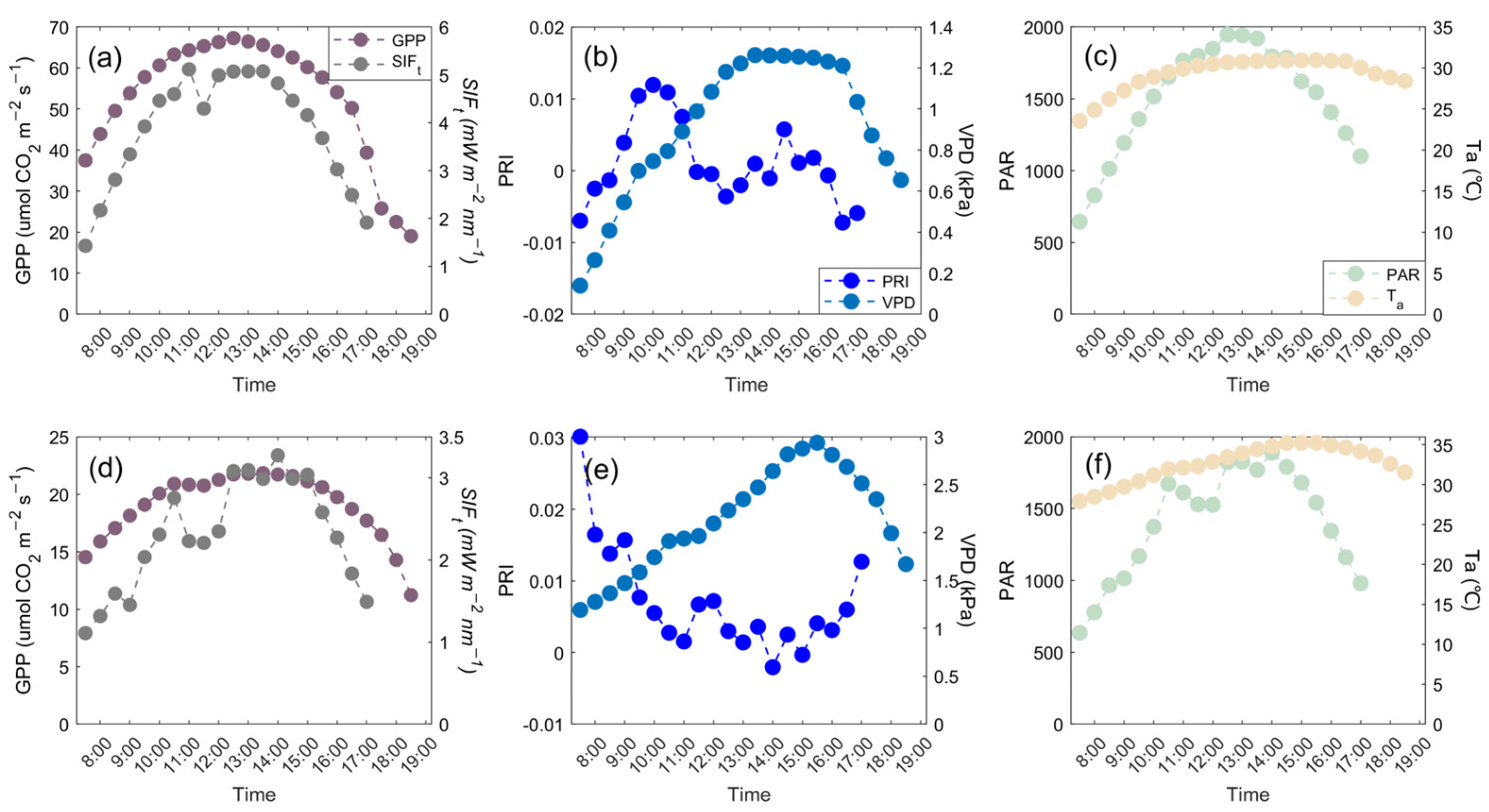
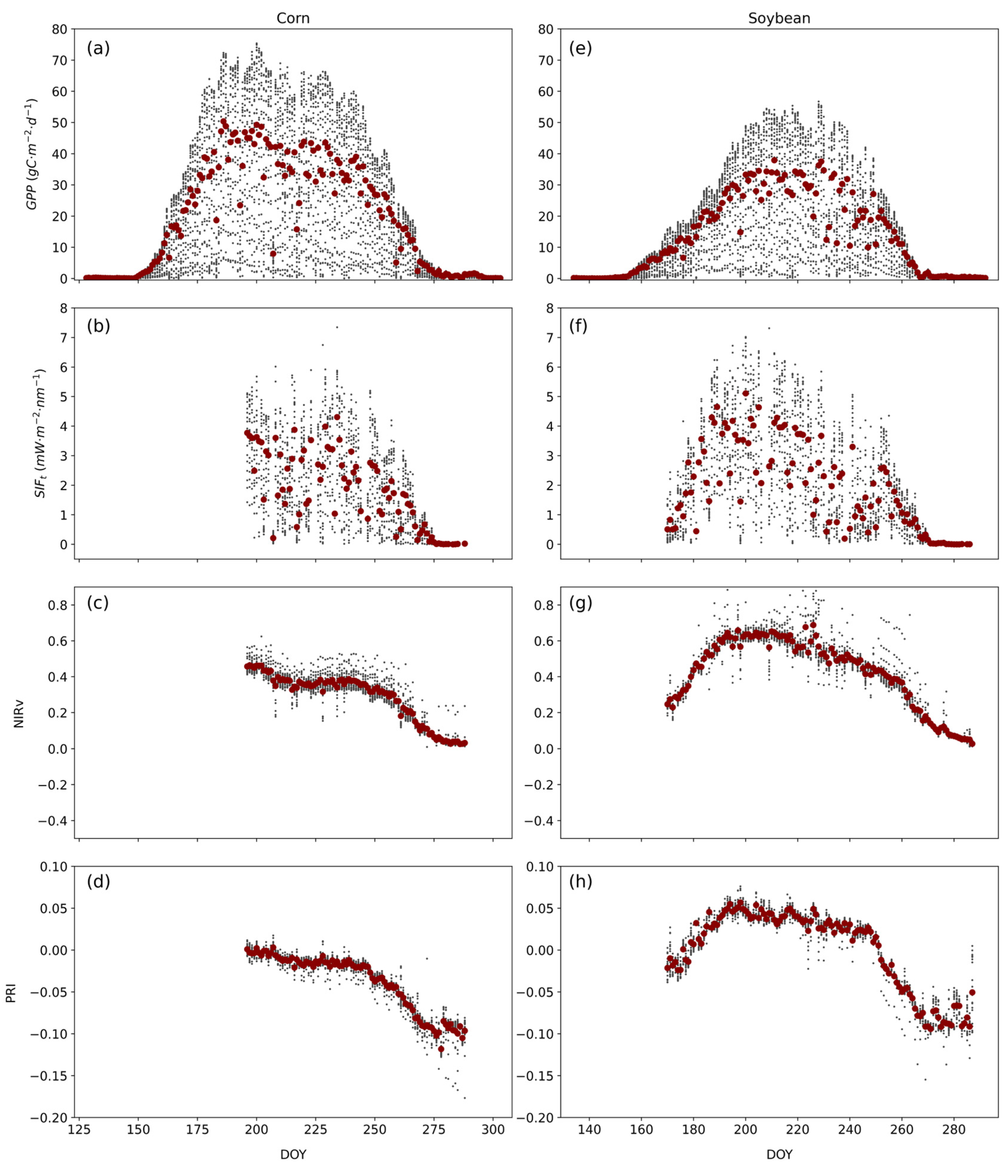
3.1.1. Seasonal Changes of PRI, SIF and GPP

Based on tower-based measurements, it is possible to identify the precise driving mechanisms for the diurnal changes in ${SIF}_t$ and GPP. At the US-N2 site, there was a “hump-shape” diurnal pattern of SIF and GPP for corn (DOY 196 in 2017) and for soybean (DOY 180 in 2018) (Figure 2a,d). Strong diurnal patterns were seen in the SIF and GPP, with a constant increase in the morning and a subsequent fall after solar noon, mostly due to incoming radiation (PAR, Figure 2c and Figure 3f). Both GPP and SIF are driven by PAR. However, PRI exhibited a “bowl-shaped” diurnal pattern. Due to that, VPD increases until the afternoon and NPQ is inversely related to PRI; it can be inferred that a relatively larger portion of energy will be dissipated by NPQ when crops suffer from stress at some extent compared to that when crops do not experience stress (Figure 2b,e). The diurnal changes of PAR and Ta were also shown in Figure 2c,f.

3.1.2. Seasonal Changes of PRI, SIF and GPP

Figure 3 displays the measured data for two consecutive growth periods (one is for corn; the other is for soybean) at the US-Ne2 site. The observed data at the US-Ne3 site can be found in Figure S1. It can be shown that for both corn and soybean, ${SIF}_t$ and GPP followed similar seasonal patterns. PRI showed an obvious seasonal shift, which may also contain information about energy allocation changes. In order to reduce the influences of chlorophyll content and canopy structure on PRI, we only used measured data at the growth peak period with NDVI greater than 0.70 for subsequent analysis.

3.2. Special Role of PRI in the SIF–GPP Relationship for Corn and Soybean

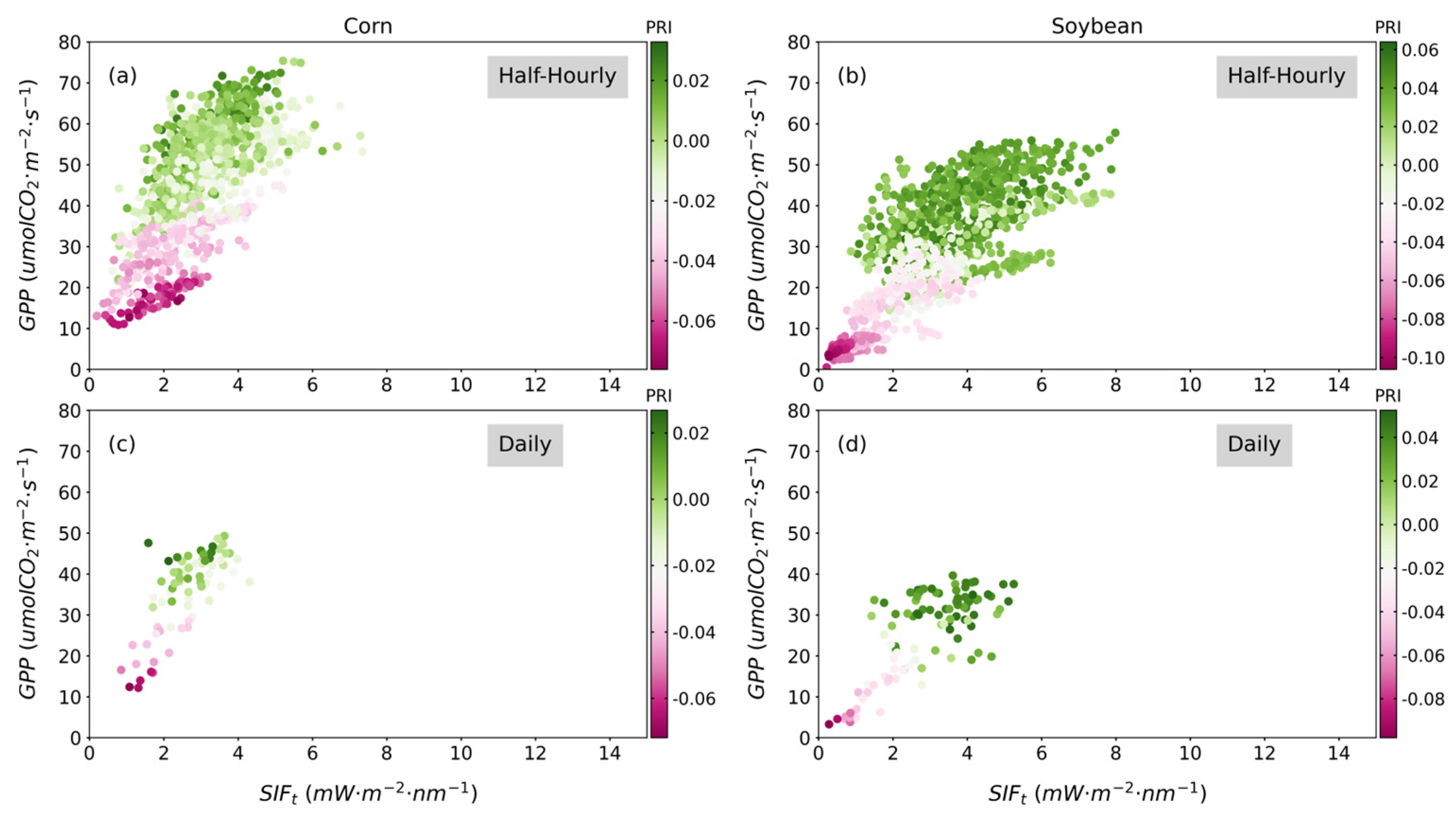
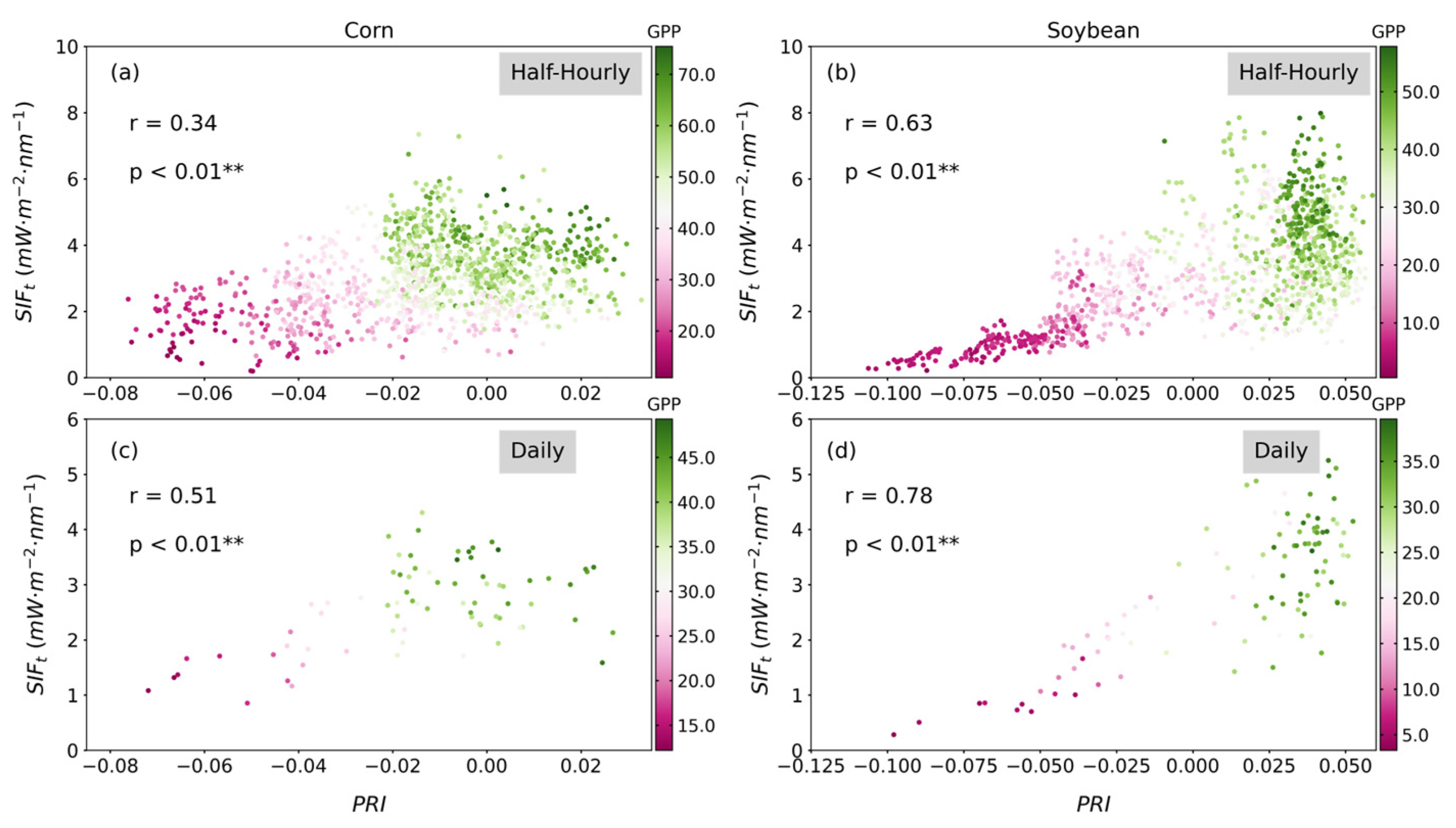
3.2.1. Linear Relationship of SIF to GPP for Corn and Soybean

For corn and soybean, we examined the association between ${SIF}_t$ and GPP. At the half-hourly and daily timescales, ${SIF}_t$ exhibited a strong connection with GPP for both corn and soybean (R² = 0.48–0.62, p < 0.01;

Table 1. Regression relationship between ${SIF}_t$ and GPP for corn and soybean. ${GPP}_{pre}$ represents the predicted GPP.

Crops	Timescale	Linear Model	R2	RMSE	r	p
Corn	Half-hourly	${GPP}_{pre}=8.87\times {SIF}_t+20.29$	0.48	10.22	0.69	<0.01
	Daily	${GPP}_{pre}=8.38\times {SIF}_t+13.93$	0.49	6.38	0.70	<0.01
Soybean	Half-hourly	${GPP}_{pre}=6.45\times {SIF}_t+8.85$	0.54	9.59	0.73	<0.01
	Daily	${GPP}_{pre}=6.57\times {SIF}_t+5.23$	0.62	6.25	0.79	<0.01

). It is worthy to note that the slope of the linear ${SIF}_t$–GPP relationship for corn ranged from 8.38 to 8.87 ($\mathsf{\mu }\mathrm{m}\mathrm{o}\mathrm{l} {\mathrm{C}\mathrm{O}}_2·{\mathrm{m}}^{-2}·{\mathrm{s}}^{-1}$), whereas the slopes for soybean ranged from 6.45 to 6.57 ($\mathsf{\mu }\mathrm{m}\mathrm{o}\mathrm{l} {\mathrm{C}\mathrm{O}}_2·{\mathrm{m}}^{-2}·{\mathrm{s}}^{-1}$).

From Figure 4, it can be seen that the slopes of the ${SIF}_t$–GPP relationship generally have a lower value at the lower PRI than that at the higher PRI. It is critical to combine information from ${SIF}_t$ and PRI in order to calculate GPP accurately.

3.2.2. Relationships between PRI and SIF for Corn and Soybean

Due to the importance of SIF and NPQ as key energy dissipation pathways other than PQ, it is crucial to comprehend the potential association between SIF and NPQ in order to more accurately estimate GPP. NPQ can be represented by PRI using remote sensing methods. At half-hourly and daily timescales, there is a substantial correlation between ${SIF}_t$ and PRI for corn and soybean (Figure 5). However, PRI has a stronger correlation with ${SIF}_t$ for soybean (0.63 for half-hourly data and 0.78 for daily data) than that for corn (0.34 for half-hourly data and 0.51 for daily data). It suggests that for soybean, SIF is more prone to be influenced by PRI.

Additionally, ${SIF}_t$ and GPP had a lower value at lower PRI (Figure 5) and the slopes of the ${SIF}_t$–GPP relationship varied with PRI (Figure 4). It indicates that the allocated energy to GPP and ${SIF}_t$ fluctuates dynamically with NPQ and the ratio of GPP to ${SIF}_t$ has a higher value when NPQ decreases. Therefore, the potential fluctuations in energy for NPQ should be taken into account in the ${SIF}_t$-based GPP estimation.

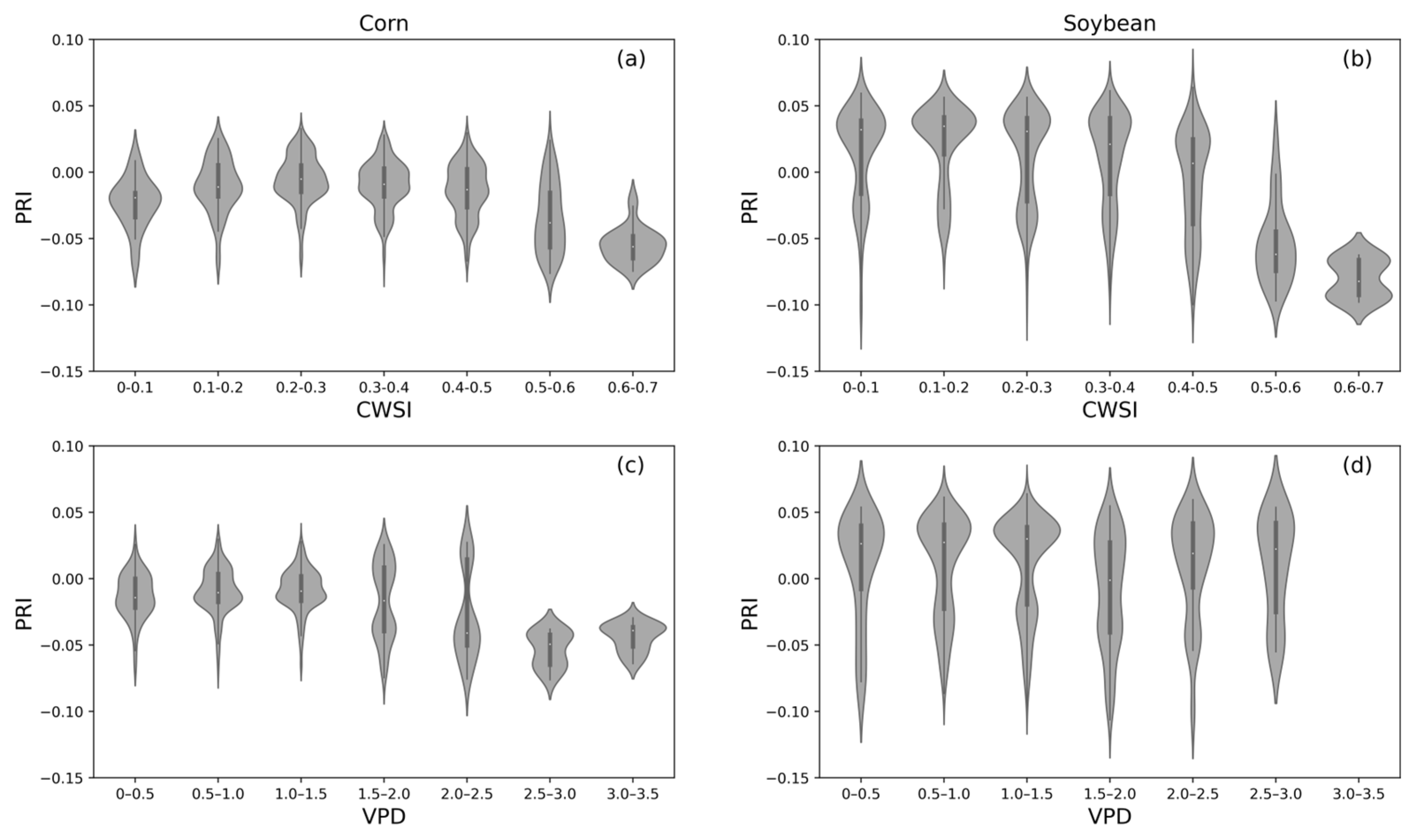
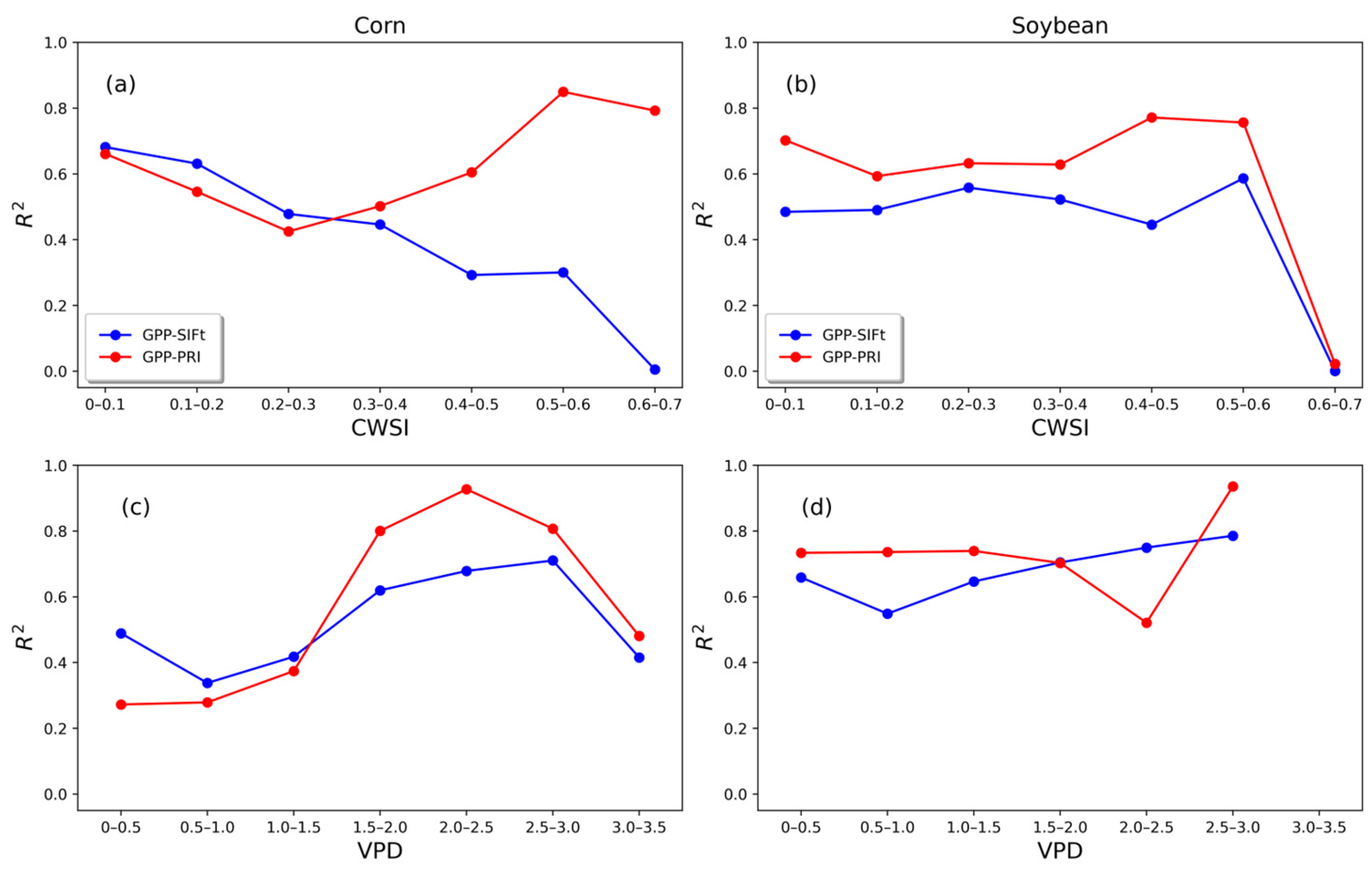
3.2.3. Impact of PRI on the SIF–GPP Relationship under Different Stress Conditions

In this study, in order to better explore the impact of PRI on the SIF–GPP relationship under different stress conditions, we considered two stress indicators, including CWSI and VPD. CWSI can reflect the stressed status of crops in response to water deficit. Water deficit affects crops’ physical–physiological activities (e.g., photosynthesis and transpiration), among which the stomatal conductance is an important adaptation mechanism to environment. Additionally, we used VPD to represent the degree of dryness of the air.

Figure 6a,b shows that for both corn and soybean, PRI falls with increasing CWSI. In reaction to stress, a plant will dissipate more energy absorbed by chlorophyll molecules through NPQ. The reduction in energy allocated for photosynthesis or the stomatal responses to stress may be the causes of GPP downregulation. As ${SIF}_t$ or NPQ are a component of the light reactions other than those that are related to the dark reactions, the incongruity of light and dark reactions is a potential factor that could influence the GPP estimation based on ${SIF}_t$ and PRI. Despite a slight decline of PRI with VPD for soybean, PRI showed an obvious decreasing tendency with increasing VPD for corn (Figure 6c,d).

In addition, using correlation coefficients, we also analyzed the impacts of CWSI and VPD on the relationships between GPP and ${SIF}_t$ as well as PRI (Figure 7). For corn and soybean, the GPP–${SIF}_t$ relationship exhibited a gradually downward trend along with CWSI (Figure 7a,b). The GPP–${SIF}_t$ relationships for corn exhibited a more pronounced decline than those for soybean with an increase in CWSI. The GPP–PRI relationship resembled a flat lying “S” shape with increasing CWSI. When CWSI was higher than 0.6, there was a downward tendency in these correlation coefficients. Figure 7c,d also depict the impact of VPD on the relationship of GPP to PRI and ${SIF}_t$.

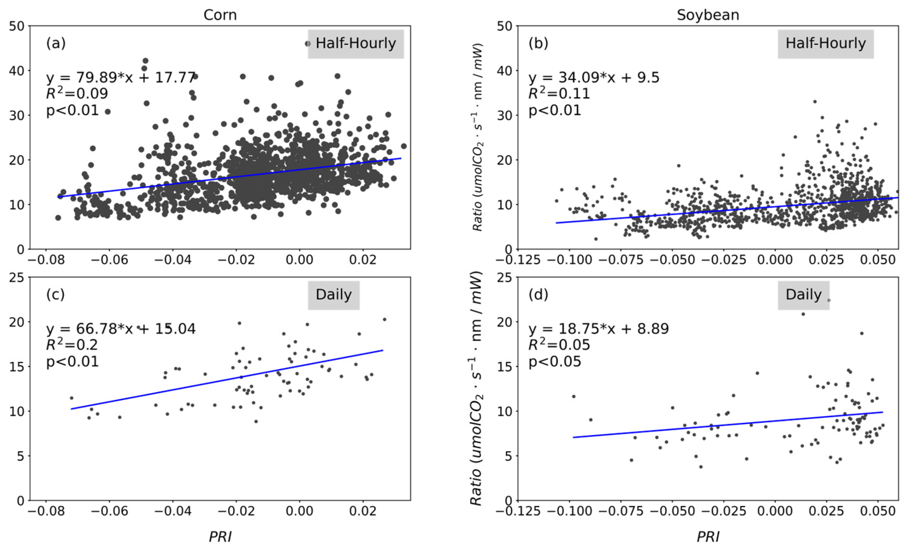
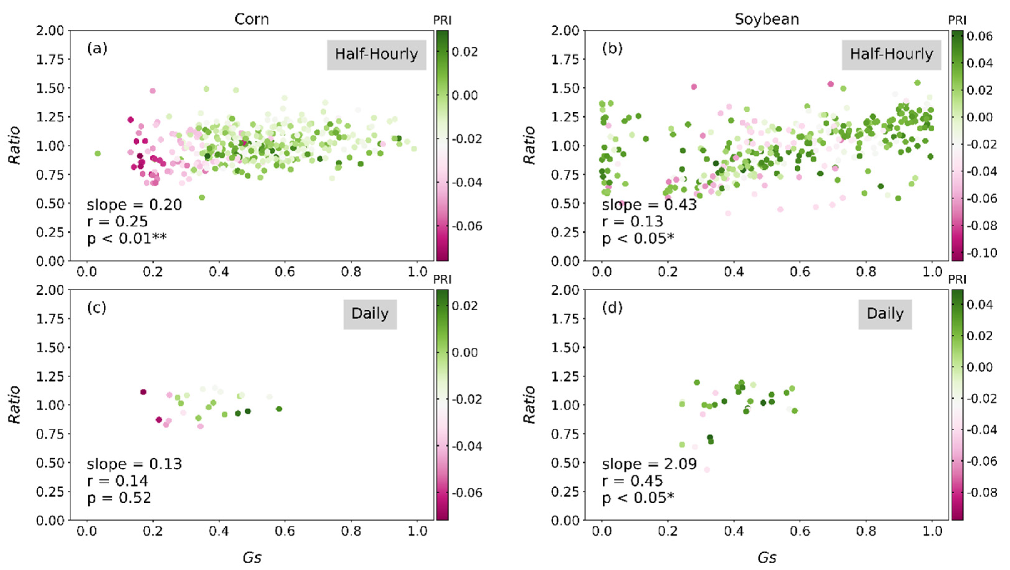
3.2.4. Partial Correlation Analysis between the Ratio of GPP to SIF and PRI

As shown by the results above, PRI plays an important role in the ${SIF}_t$–GPP relationship. For corn and soybean, the ratio of GPP to ${SIF}_t$ increases with PRI (Figure 8). In contrast to soybean, corn showed a clear upward tendency of the ratio of GPP to ${SIF}_t$ with PRI. It can be interpreted that ${SIF}_t$ is more sensitive to PRI for soybean (Figure 8) and that the division of GPP by SIF reduces some impacts of PRI on the ratio of GPP to ${SIF}_t$ for soybean.

It is worthy to note that complex structural-physiological factors and environmental factors have an influence on the ${SIF}_t$–GPP relationship. To better interpreter the potential impact of PRI on the ${SIF}_t$–GPP relationship, the correlation of PRI with the ratio of GPP to ${SIF}_t$ and its relationship to other influencing variables should be analyzed in detail.

In this study, we used Partial correlation analysis to distinguish the impacts of environmental variables (PAR, Ta, VPD, CWSI) and structural-physiological factors (Gs, NIRv, NDVI) on the relationship of PRI and the ratio of GPP to ${SIF}_t$ (

Table 2. Correlation coefficients for the links between PRI and the ratio of GPP to ${SIF}_t$ for corn and soybean at half-hourly timescales. The control variables are included in parenthesis, and the Pearson and Partial correlation coefficients are provided.

Crops	Timescales	Pearson’s Coefficient of Correlation	Partial Correlation Coefficient
			Physiology	Structure		Environment
			(Gs)	(NIRv)	(NDVI)	(PAR)	(Ta)	(VPD)	(CWSI)
Corn	Half-hourly	0.31 **	0.33 **	0.02	0.28 **	0.45 **	0.30 **	0.26 **	0.27 **
	Daily	0.45 **	0.51 **	0.23 *	0.56 **	0.56 **	0.41 **	0.47 **	0.45 **
Soybean	Half-hourly	0.33 **	0.31 **	0.13 **	0.06 *	0.45 **	0.45 **	0.33 **	0.25 **
	Daily	0.22 *	0.19 *	0.24 *	–0.02	0.45 **	0.34 **	0.18	0.23 *

“*” is the significance level of 0.05 and “**” represents the significance level of 0.01.

). By controlling the structural variables (NIRv, NDVI), the PRI is less strongly correlated with the ratio of GPP to ${SIF}_t$ than it is with other variables (Gs, PAR, etc.). It can be explained by the fact that PRI contains some information about structure or chlorophyll content. In addition, NDVI or NIRv is also related to leaf growth and leaf age, which affect the dynamic variations in NPQ. It should be noted that the relationships between the ratio of GPP to ${SIF}_t$ and PRI were significant when Gs was controlled for both corn and soybean, which may be due to the fact that PRI contains some information about plant responses to stress (Figure 6) and that there was no severe stress for the crops that could have caused an imbalance between the light and dark reactions. Overall, the relationships between PRI and the ratio of GPP to ${SIF}_t$ were almost all significant in both the Partial and Pearson correlation analyses, regardless of controlling structural-physiological and environmental variables.

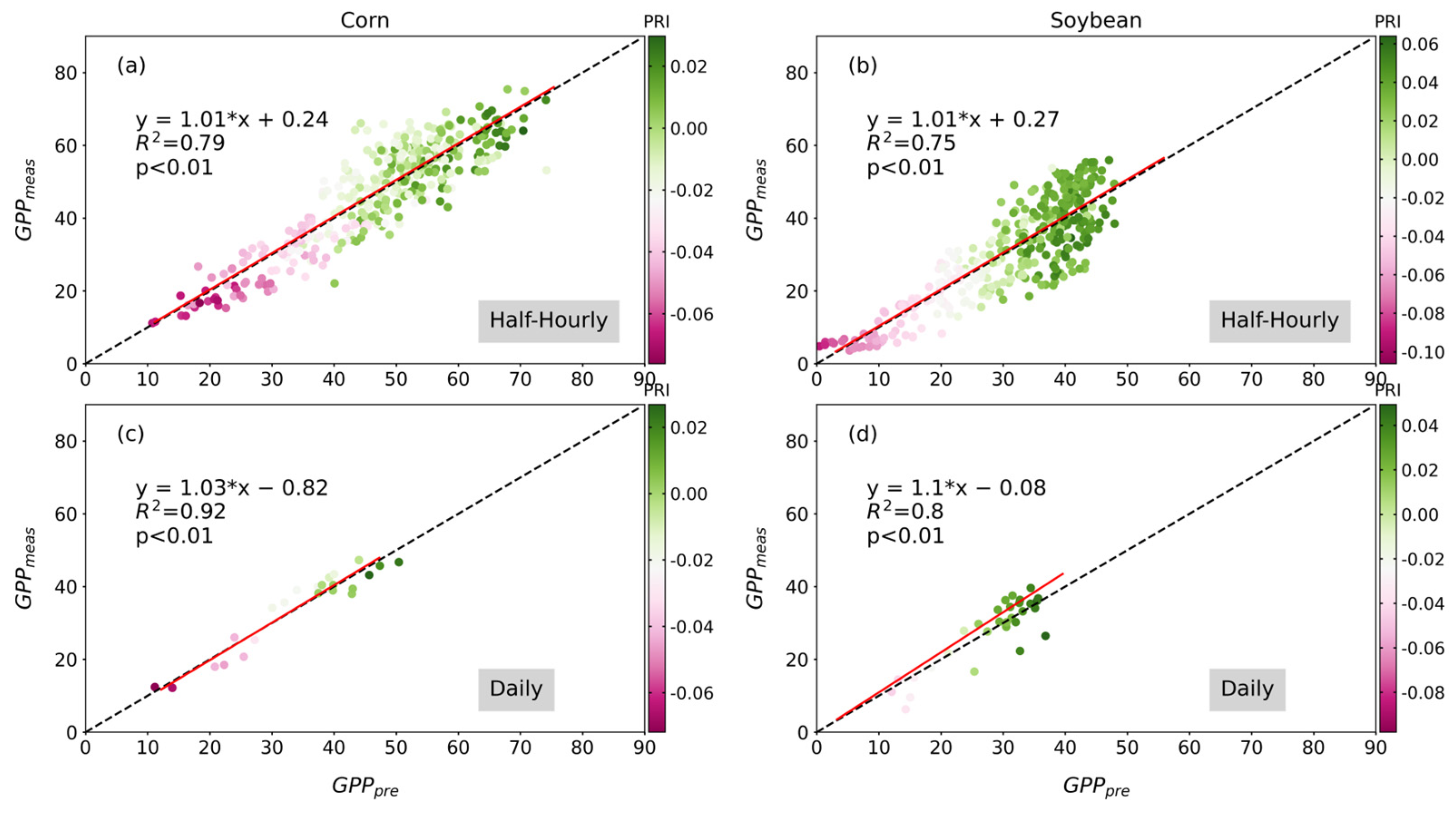
3.3. Improvement of GPP Estimation Using a Combination of SIF and PRI for Corn and Soybean

At half-hourly and daily timescales, the impact of PRI on the ${SIF}_t$–GPP relationship was evaluated for corn and soybean. The measured data was randomly divided into two parts: 70% of the measured data is utilized for modeling and the remaining 30% of the measured data is performed for validation. The multi-variable regression results are displayed in

Table 3. Multiple-variable GPP regression model based on SIF and PRI.

Crops	Timescale	Multi-Variable Linear Model	R2	RMSE	p
Corn	Half-hourly	$GPP=6.32\times {SIF}_t+389.88\times PRI+32.71$	0.78	6.60	<0.01
	Daily	$GPP=4.89\times {SIF}_t+287.46\times PRI+27.01$	0.84	3.56	<0.01
Soybean	Half-hourly	$GPP=2.87\times {SIF}_t+230.13\times PRI+19.00$	0.78	6.60	<0.01
	Daily	$GPP=0.95\times {SIF}_t+218.85\times PRI+19.39$	0.82	4.34	<0.01

. After combining ${SIF}_t$ and PRI, the slopes between GPP and ${SIF}_t$ for corn (4.89–6.32) were also higher than those for soybean (0.95–2.87), and there is a good GPP estimation accuracy with higher R² values (0.78) and lower RMSE (6.60 $\mathsf{\mu }\mathrm{m}\mathrm{o}\mathrm{l} {\mathrm{C}\mathrm{O}}_2·{\mathrm{m}}^{-2}{\mathrm{s}}^{-1}$) at half-hourly timescales as well as with higher R² values (0.82–0.84) and lower RMSE (3.56–4.3 $\mathsf{\mu }\mathrm{m}\mathrm{o}\mathrm{l} {\mathrm{C}\mathrm{O}}_2·{\mathrm{m}}^{-2}{\mathrm{s}}^{-1}$) at daily timescales. These results suggest that fluorescence and PRI should be considered in the GPP estimation model.

It is worthy to note that the slope of the ${SIF}_t$–GPP relationship differs between corn (a C4 crop) and soybean (a C3 crop), with a higher slope for corn than that for soybean. In comparison to the GPP estimation model based solely on ${SIF}_t$, the GPP estimation model based on both ${SIF}_t$ and PRI has a lower value of fitted coefficients between ${SIF}_t$ and GPP (Table 1 and Table 3).

The remaining 30% of the data was used for validating the above equations. Figure 9 shows the relationships between true GPP obtained from EC measurements (${GPP}_{meas}$) and the modeled GPP (${GPP}_{pre}$). At half-hourly and daily timescales, the slopes of the regression lines for both corn and soybean were approximately equal to 1. There are higher R² values for corn (0.79–0.92) and soybean (0.75–0.80). Therefore, PRI can be used to improve the ${SIF}_t$-based GPP estimation.

In addition, we investigate the effects of Gs on the GPP estimation. From Figure 10, we can see that the ratio of ${GPP}_{meas}$ to ${GPP}_{pre}$ correlated to Gs for corn (r = 0.25, p < 0.01) and soybean (r = 0.13, p < 0.05) at half-hourly timescales. The effects of soil water content (SWC) on the GPP estimation can be found in Figure S4. At daily timescales, the ratio of ${GPP}_{meas}$ to ${GPP}_{pre}$ was not correlated with Gs for corn (r = 0.14, p = 0.52), while it was relatively significantly related to Gs for soybean (r = 0.45, p < 0.05).

4. Discussion

4.1. Uncertainties of the GPP Estimation Based on PRI and SIF

In this study, we assessed the potential of PRI to improve the relationship between SIF and GPP for corn and soybean. The relationships of GPP to SIF and PRI are influenced by structural and physical-physiological factors. Canopy structure affects the estimation of $f_{esc}$, which further affects the estimates of the total SIF [8]. The canopy-observed SIF at a solid viewing angle has an angle effect. Therefore, it is necessary to convert the canopy-observed SIF at a solid viewing angle into the total SIF at the hemisphere [4]. Although the ratio of NIRv to fPAR can be as an approximation of the $f_{esc}$ at the near-infrared band, the influences of complex structure and soil background on the $f_{esc}$ have not been well explored [7,11]. In addition, a single-wavelength SIF cannot well characterize the broadband SIF covering the 650 nm to 800 nm spectral range [35]. The observed SIF not only contains contributions from PSII but also from PSI, while only SIF emitted from PSII is directly related to light reactions. Hitherto, there are no methods available to distinguish PSI and PSII fluorescence at leaf or canopy levels [6]. In this study, to lessen the impact of the canopy structure, we only explored the GPP–${SIF}_t$ relationships using data with NDVI greater than 0.7.

This study used PRI as an indicator of NPQ, which has demonstrated that PRI can track the dynamic changes of NPQ in previous studies, especially at short-time timescales [44]. Although this study assessed the role of PRI in regulating the SIF–GPP relationship, it depends on whether PRI is a good proxy for NPQ. Due to the fact that there are three main energy dissipated pathways, it is reasonable to combine the information from SIF and NPQ to improve GPP estimation. The intricate interplay of environmental factors (e.g., air temperature, light intensity, and water availability) have an impact on how SIF and NPQ are linked to GPP. NPQ and SIF tend to increase with PAR [45]. Low temperature may cause NPQ to increase whereas SIF may show a fall trend, provided that it does not cause damage to chlorophyll molecules [19]. According to some studies conducted in hot environments, the NPQ rises as temperature rises but SIF exhibits the opposite pattern [45,46]. Moreover, water stress made NPQ increase and might decrease SIF [47,48]. Overall, SIF and NPQ react differently to variable environmental conditions, and they have a comprehensive impact on PQ changes. As a result, the combination of SIF and NPQ has a special ability to indicate PQ dynamics under complex environmental conditions.

It is worthy to note that the decoupling of light reactions and dark reactions in response to stress may also alter the relationships of GPP to NPQ and SIF [35]. The stomatal conductance controlling the sink of CO₂ and the loss of H₂O may be more sensitive to stress conditions than the light reactions. Helm et al. [47] found that the stomata responded sensitively to the water deficit, as demonstrated by the stomatal conductance and the net photosynthetic carbon assimilation that decreased, whereas the SIF responded to water stress in eastern cottonwood less strongly. Kimm et al. [46] reported that both fluorescence quantum efficiency and stomatal conductance declined in response to water stress and NPQ exhibited an upregulated trend [15]. Magney et al. [19] found that the SIF yield showed a substantial reduction in the winter due to sustained NPQ and deactivation of the photosystems. Under stress, chlorophyll molecules typically are unable to fully utilize the solar energy they have taken in for CO₂ fixation. The photochemical activities will be damaged if the additional absorbed energy cannot be efficiently dissipated [31]. NPQ generally upregulated in response to environmental stress, while Gs showed a down-regulated trend under stress conditions [35]. The rate at which the products of electron transport—ATP and NADPH—are consumed in the dark processes is influenced by the CO₂ partial pressure in the stroma, which is determined by CO₂ diffusional resistances in the stomata and mesophylls. Feedback from the dark to light processes may therefore have an impact on how much energy is distributed across PQ, SIF, and NPQ [6]. It indicates that NPQ not only regulates the quantum yield of photochemistry and fluorescence quantum efficiency occurring in light reactions, but also can reflect some information of dark reaction in response to stress conditions. In this study, the ratio of ${GPP}_{meas}$ to ${GPP}_{meas}$ was related to Gs for corn (r = 0.25, p < 0.01) and soybean (r = 0.13, p < 0.05) at half-hourly timescales (Figure 10). Therefore, the relationships of GPP to SIF and PRI are affected by the plant physiological status in response to stress conditions, especially the incongruity of dark reactions and light reactions.

The regulated NPQ was affected by the xanthophyll cycle, which can be detected by canopy reflectance of 531 nm at short-time timescales [22]. However, the seasonal variations in PRI were largely influenced by changes in pigment pools (e.g., chlorophyll content) and the reliability of using PRI to indicate NPQ needs to be further investigated. Magney et al. [19] reported that the plant adaptation to winter not only corresponds to the changes in the xanthophyl cycle, but also variation of a variety of carotenoids (e.g., lutein and beta-carotene), which may play a photoprotective role for plants in response to low temperature. The intricate interplay of environmental factors (e.g., air temperature, light intensity, and water availability) have an impact on how SIF and PRI are linked to GPP [33,47]. Moreover, the canopy reflectance was influenced by the solar viewing geometry, canopy structure and soil background, which further affects the calculation of the PRI and the linkage of PRI to NPQ [49]. In this study, we found that the slopes of the ${SIF}_t$–GPP relationship change with PRI using tower-based measurements (Figure 4). PRI can be used to improve the ${SIF}_t$-based GPP estimation (Figure 9). Nevertheless, the potential underlying mechanisms for linking PRI to NPQ at canopy scale need to be explored further.

4.2. Limitations and Implications

In this study, we found that corn showed a more prone upward trend in the ratio of GPP to ${SIF}_t$ with rising PRI than soybean (Figure 5 and Figure 8). The SIF–GPP relationship’s slope varies depending on the biome or plant functional type (PFT), according to a number of recent research [3,4,50,51,52,53,54]. The photosynthesis of C3 and C4 plants, for instance, showed different patterns in response to environmental conditions. Because C4 plants have evolved from the C4 route to adapt to high light intensity, high temperature, and dryness through C4 photosynthesis, they have improved resource-use efficiency and potential productivity. C4 crops are more suited to warm climates than C3 crops are, and they can withstand greater temperatures and stronger light [9]. The SIF–GPP relationship was highly dependent on the PFT. In addition, as different varieties may respond differently to environmental factors, it would be beneficial to consider the effects of the specific cultivars or genotypes [55,56,57]. Overall, it suggests that different PFTs may perform differently when utilizing PRI to enhance the ${SIF}_t$–GPP relationship. In addition, although this study has demonstrated that PRI can be used to improve the ${SIF}_t$-based GPP estimation, the results were only applicable to two crops, one is corn and the other is soybean. The separation of sunlit/shaded and diffuse/direct beam radiation among the multilayer canopy structure is important for understanding the relationships of GPP to SIF and PRI [7,35]. To comprehend and forecast the complicated dynamics of SIF emission, more efforts will be required.

In this study, we used CWSI and VPD to assess the effects of stress conditions on the GPP estimation based on ${SIF}_t$ and PRI. The results show that the GPP–${SIF}_t$ and GPP–PRI relationships are influenced by environmental stress (Figure 6; Table 2). However, the influences of the environmental stress on the GPP estimation based on PRI and ${SIF}_t$ should be further investigated from leaf to canopy scales [18,43]. Therefore, in order to develop a more accurate GPP estimation model, more leaf and canopy observation experiments should be carried out in the future.

5. Conclusions

In this study, based on tower-based measurements for corn (a C4 crop) and soybean (a C3 crop), we investigated the special role of PRI in improving the ${SIF}_t$-based GPP estimation at half-hourly and daily timescales. Drought stress, as reflected by CWSI and VPD, has an impact on the coupling of GPP to ${SIF}_t$ and PRI. Corn showed a more pronounced upward trend in the ratio of GPP to ${SIF}_t$ with rising PRI than soybean. Whether in Pearson or Partial correlation analysis, the relationships of PRI to the ratio of GPP to ${SIF}_t$ were almost all significant, regardless of controlling structural-physiological (stomatal conductance, vegetation indices) and environmental variables (light intensity, temperature, etc.). Therefore, PRI has a significant influence on the ${SIF}_t$–GPP relationship for corn and soybean. In order to develop a more accurate GPP estimation model, the better proxy of NPQ should be explored in addition to PRI and more leaf and canopy observation experiments should be carried out in the future.

References

1. Beer, C.; Reichstein, M.; Tomelleri, E.; Ciais, P.; Jung, M.; Carvalhais, N.; Rödenbeck, C.; Arain, M.A.; Baldocchi, D.; Bonan, G.B. Terrestrial Gross Carbon Dioxide Uptake: Global Distribution and Covariation with Climate. Science 2010, 329, 834–838. [Google Scholar] [CrossRef] [PubMed]
2. Jeong, S.; Ryu, Y.; Dechant, B.; Li, X.; Kong, J.; Choi, W.; Kang, M.; Yeom, J.; Lim, J.; Jang, K. Tracking Diurnal to Seasonal Variations of Gross Primary Productivity Using a Geostationary Satellite, GK-2A Advanced Meteorological Imager. Remote Sens. Environ. 2023, 284, 113365. [Google Scholar] [CrossRef]
3. Sun, Y.; Wen, J.; Gu, L.; Joiner, J.; Chang, C.Y.; van Der Tol, C.; Porcar-Castell, A.; Magney, T.; Wang, L.; Hu, L.; et al. From Remotely-Sensed Solar-Induced Chlorophyll Fluorescence to Ecosystem Structure, Function, and Service: Part II-Harnessing Data. Glob. Chang. Biol. 2023, 29, 2893–2925. [Google Scholar] [CrossRef] [PubMed]
4. Guanter, L.; Bacour, C.; Schneider, A.; Aben, I.; van Kempen, T.A.; Maignan, F.; Retscher, C.; Köhler, P.; Frankenberg, C.; Joiner, J. The TROPOSIF Global Sun-Induced Fluorescence Dataset from the Sentinel-5P TROPOMI Mission. Earth Syst. Sci. Data 2021, 13, 5423–5440. [Google Scholar] [CrossRef]
5. Baker, N.R. Chlorophyll Fluorescence: A Probe of Photosynthesis in Vivo. Annu. Rev. Plant Biol. 2008, 59, 89–113. [Google Scholar] [CrossRef] [PubMed]
6. Gu, L.; Han, J.; Wood, J.D.; Chang, C.Y.-Y.; Sun, Y. Sun-induced Chl Fluorescence and Its Importance for Biophysical Modeling of Photosynthesis Based on Light Reactions. New Phytol. 2019, 223, 1179–1191. [Google Scholar] [CrossRef] [PubMed]
7. Dechant, B.; Ryu, Y.; Badgley, G.; Köhler, P.; Rascher, U.; Migliavacca, M.; Zhang, Y.; Tagliabue, G.; Guan, K.; Rossini, M. NIRVP: A Robust Structural Proxy for Sun-Induced Chlorophyll Fluorescence and Photosynthesis across Scales. Remote Sens. Environ. 2022, 268, 112763. [Google Scholar] [CrossRef]
8. Liu, X.; Guanter, L.; Liu, L.; Damm, A.; Malenovsky, Z.; Rascher, U.; Peng, D.; Du, S.; Gastellu-Etchegorry, J.-P. Downscaling of Solar-Induced Chlorophyll Fluorescence from Canopy Level to Photosystem Level Using a Random Forest Model. Remote Sens. Environ. 2019, 231, 110772. [Google Scholar] [CrossRef]
9. Liu, L.; Guan, L.; Liu, X. Directly Estimating Diurnal Changes in GPP for C3 and C4 Crops Using Far-Red Sun-Induced Chlorophyll Fluorescence. Agric. For. Meteorol. 2017, 232, 1–9. [Google Scholar] [CrossRef]
10. Badgley, G.; Field, C.B.; Berry, J.A. Canopy Near-Infrared Reflectance and Terrestrial Photosynthesis. Sci. Adv. 2017, 3, e1602244. [Google Scholar] [CrossRef] [PubMed]
11. Braghiere, R.K.; Wang, Y.; Doughty, R.; Sousa, D.; Magney, T.; Widlowski, J.-L.; Longo, M.; Bloom, A.A.; Worden, J.; Gentine, P. Accounting for Canopy Structure Improves Hyperspectral Radiative Transfer and Sun-Induced Chlorophyll Fluorescence Representations in a New Generation Earth System Model. Remote Sens. Environ. 2021, 261, 112497. [Google Scholar] [CrossRef]
12. Yang, P.; van der Tol, C. Linking Canopy Scattering of Far-Red Sun-Induced Chlorophyll Fluorescence with Reflectance. Remote Sens. Environ. 2018, 209, 456–467. [Google Scholar] [CrossRef]
13. Zeng, Y.; Badgley, G.; Dechant, B.; Ryu, Y.; Chen, M.; Berry, J.A. A Practical Approach for Estimating the Escape Ratio of Near-Infrared Solar-Induced Chlorophyll Fluorescence. Remote Sens. Environ. 2019, 232, 111209. [Google Scholar] [CrossRef]
14. Rajewicz, P.A.; Zhang, C.; Atherton, J.; Van Wittenberghe, S.; Riikonen, A.; Magney, T.; Fernandez-Marin, B.; Plazaola, J.I.G.; Porcar-Castell, A. The Photosynthetic Response of Spectral Chlorophyll Fluorescence Differs across Species and Light Environments in a Boreal Forest Ecosystem. Agric. For. Meteorol. 2023, 334, 109434. [Google Scholar] [CrossRef]
15. Chen, J.; Liu, X.; Du, S.; Ma, Y.; Liu, L. Effects of Drought on the Relationship between Photosynthesis and Chlorophyll Fluorescence for Maize. IEEE J. Sel. Top. Appl. Earth Obs. Remote Sens. 2021, 14, 11148–11161. [Google Scholar] [CrossRef]
16. Chen, J.; Liu, X.; Ma, Y.; Liu, L. Effects of Low Temperature on the Relationship between Solar-Induced Chlorophyll Fluorescence and Gross Primary Productivity across Different Plant Function Types. Remote Sens. 2022, 14, 3716. [Google Scholar] [CrossRef]
17. Wu, G.; Jiang, C.; Kimm, H.; Wang, S.; Bernacchi, C.; Moore, C.E.; Suyker, A.; Yang, X.; Magney, T.; Frankenberg, C.; et al. Difference in Seasonal Peak Timing of Soybean Far-Red SIF and GPP Explained by Canopy Structure and Chlorophyll Content. Remote Sens. Environ. 2022, 279, 113104. [Google Scholar] [CrossRef]
18. Wang, X.; Chen, J.M.; Ju, W. Photochemical Reflectance Index (PRI) can Be Used to Improve the Relationship between Gross Primary Productivity (GPP) and Sun-Induced Chlorophyll Fluorescence (SIF). Remote Sens. Environ. 2020, 246, 111888. [Google Scholar] [CrossRef]
19. Magney, T.S.; Bowling, D.R.; Logan, B.A.; Grossmann, K.; Stutz, J.; Blanken, P.D.; Burns, S.P.; Cheng, R.; Garcia, M.A.; Kohler, P.; et al. Mechanistic Evidence for Tracking the Seasonality of Photosynthesis with Solar-Induced Fluorescence. Proc. Natl. Acad. Sci. USA 2019, 116, 11640–11645. [Google Scholar] [CrossRef] [PubMed]
20. Sukhova, E.; Sukhov, V. Connection of the Photochemical Reflectance Index (PRI) with the Photosystem II Quantum Yield and Nonphotochemical Quenching Can Be Dependent on Variations of Photosynthetic Parameters among Investigated Plants: A Meta-Analysis. Remote Sens. 2018, 10, 771. [Google Scholar] [CrossRef]
21. Gitelson, A.; Viña, A.; Solovchenko, A.; Arkebauer, T.; Inoue, Y. Derivation of Canopy Light Absorption Coefficient from Reflectance Spectra. Remote Sens. Environ. 2019, 231, 111276. [Google Scholar] [CrossRef]
22. Gitelson, A.A.; Gamon, J.A.; Solovchenko, A. Multiple Drivers of Seasonal Change in PRI: Implications for Photosynthesis 2. Stand Level. Remote Sens. Environ. 2017, 190, 198–206. [Google Scholar] [CrossRef]
23. Du, S.; Liu, X.; Chen, J.; Duan, W.; Liu, L. Addressing Validation Challenges for TROPOMI Solar-Induced Chlorophyll Fluorescence Products Using Tower-Based Measurements and an NIRv-Scaled Approach. Remote Sens. Environ. 2023, 290, 113547. [Google Scholar] [CrossRef]
24. Miao, G.; Guan, K.; Yang, X.; Bernacchi, C.J.; Berry, J.A.; DeLucia, E.H.; Wu, J.; Moore, C.E.; Meacham, K.; Cai, Y.; et al. Sun-Induced Chlorophyll Fluorescence, Photosynthesis, and Light Use Efficiency of a Soybean Field from Seasonally Continuous Measurements. J. Geophys. Res. Biogeosci. 2018, 123, 610–623. [Google Scholar] [CrossRef]
25. Drusch, M.; Moreno, J.; Del Bello, U.; Franco, R.; Goulas, Y.; Huth, A.; Kraft, S.; Middleton, E.M.; Miglietta, F.; Mohammed, G.; et al. The FLuorescence EXplorer Mission Concept-ESA’s Earth Explorer 8. IEEE Trans. Geosci. Remote Sens. 2017, 55, 1273–1284. [Google Scholar] [CrossRef]
26. Wu, G.; Guan, K.; Kimm, H.; Miao, G.; Jiang, C. SIF and Vegetation Indices in the US Midwestern Agroecosystems, 2016–2021; ORNL DAAC: Oak Ridge, TN, USA, 2023. [Google Scholar]
27. Wu, G.; Guan, K.; Jiang, C.; Kimm, H.; Miao, G.; Yang, X.; Bernacchi, C.J.; Sun, X.; Suyker, A.E.; Moore, C.E. Can Upscaling Ground Nadir SIF to Eddy Covariance Footprint Improve the Relationship between SIF and GPP in Croplands? Agric. For. Meteorol. 2023, 338, 109532. [Google Scholar] [CrossRef]
28. Hu, J.; Liu, L.; Guo, J.; Du, S.; Liu, X. Upscaling Solar-Induced Chlorophyll Fluorescence from an Instantaneous to Daily Scale Gives an Improved Estimation of the Gross Primary Productivity. Remote Sens. 2018, 10, 1663. [Google Scholar] [CrossRef]
29. Suyker, A.E.; Verma, S.B. Gross Primary Production and Ecosystem Respiration of Irrigated and Rainfed Maize-Soybean Cropping Systems over 8 Years. Agric. For. Meteorol. 2012, 165, 12–24. [Google Scholar] [CrossRef]
30. Porcar-Castell, A. A High-Resolution Portrait of the Annual Dynamics of Photochemical and Non-Photochemical Quenching in Needles of Pinus Sylvestris. Physiol. Plant. 2011, 143, 139–153. [Google Scholar] [CrossRef] [PubMed]
31. Porcar-Castell, A.; Malenovsky, Z.; Magney, T.; Van Wittenberghe, S.; Fernandez-Marin, B.; Maignan, F.; Zhang, Y.; Maseyk, K.; Atherton, J.; Albert, L.P.; et al. Chlorophyll a Fluorescence Illuminates a Path Connecting Plant Molecular Biology to Earth-System Science. Nat. Plants 2021, 7, 998–1009. [Google Scholar] [CrossRef] [PubMed]
32. Chang, C.Y.; Guanter, L.; Frankenberg, C.; Köhler, P.; Gu, L.; Magney, T.S.; Grossmann, K.; Sun, Y. Systematic Assessment of Retrieval Methods for Canopy Far-red Solar-induced Chlorophyll Fluorescence Using High-frequency Automated Field Spectroscopy. J. Geophys. Res. Biogeosci. 2020, 125, e2019JG005533. [Google Scholar] [CrossRef]
33. Wu, L.; Zhang, X.; Rossini, M.; Wu, Y.; Zhang, Z.; Zhang, Y. Physiological Dynamics Dominate the Response of Canopy Far-Red Solar-Induced Fluorescence to Herbicide Treatment. Agric. For. Meteorol. 2022, 323, 109063. [Google Scholar] [CrossRef]
34. Zhang, Z.; Zhang, Y.; Porcar-Castell, A.; Joiner, J.; Guanter, L.; Yang, X.; Migliavacca, M.; Ju, W.; Sun, Z.; Chen, S.; et al. Reduction of Structural Impacts and Distinction of Photosynthetic Pathways in a Global Estimation of GPP from Space-Borne Solar-Induced Chlorophyll Fluorescence. Remote Sens. Environ. 2020, 240, 111722. [Google Scholar] [CrossRef]
35. Sun, Y.; Gu, L.; Wen, J.; van Der Tol, C.; Porcar-Castell, A.; Joiner, J.; Chang, C.Y.; Magney, T.; Wang, L.; Hu, L.; et al. From Remotely Sensed Solar-Induced Chlorophyll Fluorescence to Ecosystem Structure, Function, and Service: Part I-Harnessing Theory. Glob. Chang. Biol. 2023, 29, 2926–2952. [Google Scholar] [CrossRef] [PubMed]
36. Cochavi, A.; Amer, M.; Stern, R.; Tatarinov, F.; Migliavacca, M.; Yakir, D. Differential Responses to Two Heatwave Intensities in a Mediterranean Citrus Orchard Are Identified by Combining Measurements of Fluorescence and Carbonyl Sulfide (COS) and CO2 Uptake. New Phytol. 2021, 230, 1394–1406. [Google Scholar] [CrossRef] [PubMed]
37. Testi, L.; Goldhamer, D.A.; Iniesta, F.; Salinas, M. Crop Water Stress Index Is a Sensitive Water Stress Indicator in Pistachio Trees. Irrig. Sci. 2008, 26, 395–405. [Google Scholar] [CrossRef]
38. Jackson, R.D.; Idso, S.B.; Reginato, R.J.; Pinter, P.J., Jr. Canopy Temperature as a Crop Water Stress Indicator. Water Resour. Res. 1981, 17, 1133–1138. [Google Scholar] [CrossRef]
39. Priestley, C.H.B.; Taylor, R.J. On the Assessment of Surface Heat Flux and Evaporation Using Large-Scale Parameters. Mon. Weather Rev. 1972, 100, 81–92. [Google Scholar] [CrossRef]
40. Zhang, K.; Kimball, J.S.; Mu, Q.; Jones, L.A.; Goetz, S.J.; Running, S.W. Satellite Based Analysis of Northern ET Trends and Associated Changes in the Regional Water Balance from 1983 to 2005. J. Hydrol. 2009, 379, 92–110. [Google Scholar] [CrossRef]
41. Li, X.; Gentine, P.; Lin, C.; Zhou, S.; Sun, Z.; Zheng, Y.; Liu, J.; Zheng, C. A Simple and Objective Method to Partition Evapotranspiration into Transpiration and Evaporation at Eddy-Covariance Sites. Agric. For. Meteorol. 2019, 265, 171–182. [Google Scholar] [CrossRef]
42. Penman, H.L. Natural Evaporation from Open Water, Hare Soil and Grass. Proc. R. Soc. Lond. Ser. A Math. Phys. Sci. 1948, 193, 120–145. [Google Scholar] [CrossRef]
43. Ma, L.; Sun, L.; Wang, S.; Chen, J.; Chen, B.; Zhu, K.; Amir, M.; Wang, X.; Liu, Y.; Wang, P.; et al. Analysis on the Relationship between Sun-Induced Chlorophyll Fluorescence and Gross Primary Productivity of Winter Wheat in Northern China. Ecol. Indic. 2022, 139, 108905. [Google Scholar] [CrossRef]
44. Chou, S.; Chen, J.M.; Yu, H.; Chen, B.; Zhang, X.; Croft, H.; Khalid, S.; Li, M.; Shi, Q. Canopy-Level Photochemical Reflectance Index from Hyperspectral Remote Sensing and Leaf-Level Non-Photochemical Quenching as Early Indicators of Water Stress in Maize. Remote Sens. 2017, 9, 794. [Google Scholar] [CrossRef]
45. Dang, C.; Shao, Z.; Huang, X.; Zhuang, Q.; Cheng, G.; Qian, J. Vegetation Greenness and Photosynthetic Phenology in Response to Climatic Determinants. Front. For. Glob. Chang. 2023, 6, 1172220. [Google Scholar] [CrossRef]
46. Kimm, H.; Guan, K.; Burroughs, C.H.; Peng, B.; Ainsworth, E.A.; Bernacchi, C.J.; Moore, C.E.; Kumagai, E.; Yang, X.; Berry, J.A.; et al. Quantifying High-temperature Stress on Soybean Canopy Photosynthesis: The Unique Role of Sun-induced Chlorophyll Fluorescence. Glob. Chang. Biol. 2021, 27, 2403–2415. [Google Scholar] [CrossRef] [PubMed]
47. Helm, L.T.; Shi, H.; Lerdau, M.T.; Yang, X. Solar-induced Chlorophyll Fluorescence and Short-term Photosynthetic Response to Drought. Ecol. Appl. 2020, 30, e02101. [Google Scholar] [CrossRef] [PubMed]
48. Lin, J.; Zhou, L.; Wu, J.; Han, X.; Zhao, B.; Chen, M.; Liu, L. Water Stress Significantly Affects the Diurnal Variation of Solar-Induced Chlorophyll Fluorescence (SIF): A Case Study for Winter Wheat. Sci. Total Environ. 2024, 908, 168256. [Google Scholar] [CrossRef] [PubMed]
49. Atherton, J.; Nichol, C.J.; Porcar-Castell, A. Using Spectral Chlorophyll Fluorescence and the Photochemical Reflectance Index to Predict Physiological Dynamics. Remote Sens. Environ. 2016, 176, 17–30. [Google Scholar] [CrossRef]
50. Guanter, L.; Zhang, Y.; Jung, M.; Joiner, J.; Voigt, M.; Berry, J.A.; Frankenberg, C.; Huete, A.R.; Zarco-Tejada, P.; Lee, J.-E.; et al. Global and Time-Resolved Monitoring of Crop Photosynthesis with Chlorophyll Fluorescence. Proc. Natl. Acad. Sci. USA 2014, 111, E1327–E1333. [Google Scholar] [CrossRef] [PubMed]
51. Damm, A.; Guanter, L.; Paul-Limoges, E.; Van Der Tol, C.; Hueni, A.; Buchmann, N.; Eugster, W.; Ammann, C.; Schaepman, M.E. Far-Red Sun-Induced Chlorophyll Fluorescence Shows Ecosystem-Specific Relationships to Gross Primary Production: An Assessment Based on Observational and Modeling Approaches. Remote Sens. Environ. 2015, 166, 91–105. [Google Scholar] [CrossRef]
52. Parazoo, N.C.; Bowman, K.; Fisher, J.B.; Frankenberg, C.; Jones, D.B.A.; Cescatti, A.; Pérez-Priego, Ó.; Wohlfahrt, G.; Montagnani, L. Terrestrial Gross Primary Production Inferred from Satellite Fluorescence and Vegetation Models. Glob. Chang. Biol. 2014, 20, 3103–3121. [Google Scholar] [CrossRef] [PubMed]
53. Verrelst, J.; Rivera, J.P.; Van Der Tol, C.; Magnani, F.; Mohammed, G.; Moreno, J. Global Sensitivity Analysis of the SCOPE Model: What Drives Simulated Canopy-Leaving Sun-Induced Fluorescence? Remote Sens. Environ. 2015, 166, 8–21. [Google Scholar] [CrossRef]
54. Liu, Z.; Zhao, F.; Liu, X.; Yu, Q.; Wang, Y.; Peng, X.; Cai, H.; Lu, X. Direct Estimation of Photosynthetic CO2 Assimilation from Solar-Induced Chlorophyll Fluorescence (SIF). Remote Sens. Environ. 2022, 271, 112893. [Google Scholar] [CrossRef]
55. De Queiroz Otone, J.D.; Theodoro, G.D.F.; Santana, D.C.; Teodoro, L.P.R.; De Oliveira, J.T.; De Oliveira, I.C.; Da Silva Junior, C.A.; Teodoro, P.E.; Baio, F.H.R. Hyperspectral Response of the Soybean Crop as a Function of Target Spot (Corynespora Cassiicola) Using Machine Learning to Classify Severity Levels. AgriEngineering 2024, 6, 330–343. [Google Scholar] [CrossRef]
56. Patinni, I.R.G.; De Andrade, C.A.; Campos, C.N.S.; Teodoro, L.P.R.; Andrade, S.M.; Roque, C.G.; Da Silva Junior, C.A.; Teodoro, P.E. Agronomic Performance and Water-use Efficiency of F3 Soybean Populations Grown under Contrasting Base Saturation. J Agron. Crop Sci. 2020, 206, 806–814. [Google Scholar] [CrossRef]
57. Santana, D.C.; Teodoro, L.P.R.; Baio, F.H.R.; Santos, R.G.D.; Coradi, P.C.; Biduski, B.; Silva Junior, C.A.D.; Teodoro, P.E.; Shiratsuchi, L.S. Classification of Soybean Genotypes for Industrial Traits Using UAV Multispectral Imagery and Machine Learning. Remote Sens. Appl. Soc. Environ. 2023, 29, 100919. [Google Scholar] [CrossRef]
Figure 1. Information of the two field sites deployed with FluoSpec2 systems. (a) The specific location for US-Ne2 and US-Ne3 sites; (b) a simple schematic diagram of a FluoSpec2 system consisted of a QEPRO spectrometer and a HR2000+ spectrometer; (c) a conceptual field deployment for spectral measurements.
Atmosphere 15 00463 g001
Figure 2. Diurnal changes of GPP (purple lines) and S I F t (grey lines) for corn ((a), DOY 196 in 2017) and soybean ((d), DOY 180 in 2018) crops at US-Ne2 sites based on tower-based measurements; (b) and (e), respectively, represents the diurnal changes of PRI (blue lines) and VPD (light bule lines) for corn and soybean; (c) and (f), respectively, indicates the diurnal changes of PAR (green lines) and Ta (yellow lines) for corn and soybean.
Atmosphere 15 00463 g002
Figure 3. Seasonal variations of GPP (a,e), S I F t (b,f), NIRv (c,g) and PRI (d,h) for corn and soybean at US-Ne2 site. The measured data at US-Ne3 site can be found in Figure S1. The black scatters represent half-hourly data, while the red ones indicate the daily-averaged data.
Atmosphere 15 00463 g003
Figure 4. Relationships between S I F t and GPP for corn ((a) for half-hourly data; (c) for daily data) and soybean ((b) for half-hourly data; (d) for daily data). Table 1 lists the corresponding regression coefficients. The color bar on the right indicates the magnitude of PRI.
Atmosphere 15 00463 g004
Figure 5. Relationships between PRI and S I F t for corn ((a) for half-hourly data; (c) for daily data) and soybean ((b) for half-hourly data; (d) for daily data). The Pearson correlation coefficient and the significance level were given. A significance level of 0.01 is represented by **. The color bar indicates the magnitude of GPP. The solid black line is the fitted curve.
Atmosphere 15 00463 g005
Figure 6. The first row shows violins of the PRI at 0.1 intervals of CWSI ((a) for corn, (b) for soybean), and the second row represents violins of the PRI at 0.5 intervals of VPD ((c) for corn, (d) for soybean).
Atmosphere 15 00463 g006
Figure 7. The influences of CWSI on the relationships between GPP and S I F t as well as PRI for corn (a) and soybean (b). (c,d) represent the effects of VPD on the relationships between GPP and S I F t as well as PRI for corn and soybean, respectively. The blue line shows the GPP– S I F t relationship, the red line shows the GPP–PRI relationship. CWSI was distinguished as a 0.1 interval. VPD was distinguished as a 0.5 interval.
Atmosphere 15 00463 g007
Figure 8. Relationships between the ratio of GPP to S I F t and PRI for corn ((a) for half-hourly data; (c) for daily data) and soybean ((b) for half-hourly data; (d) for daily data). The blue line is the trend line, and the shaded area represents the 95% confidence interval.
Atmosphere 15 00463 g008
Figure 9. Validation of the GPP estimation accuracy based on S I F t and PRI at half-hourly and daily timescales. G P P m e a s represents the EC measured GPP. G P P p r e represents the GPP predicted by S I F t and PRI. The validation findings for corn at half-hourly and daily timescales are shown in (a,c), respectively. (b,d) illustrate the results for soybean at half-hourly and daily timescales, respectively. The PRI value is depicted by the color bar. The best-fit line is shown by the solid red line, while the short-dashed line is the 1:1 line.
Atmosphere 15 00463 g009
Figure 10. Relationship between the ratio of G P P m e a s to G P P m e a s and Gs based on the validated dataset. (a,c) represent the relationship between the ratio to Gs for corn at half-hourly and daily timescales, respectively, while (b,d) indicate the relationship between the ratio to Gs for soybean at half-hourly and daily timescales. The color bar indicates the magnitude of PRI. “*” is the significance level of 0.05 and “**” represents the significance level of 0.01.
Atmosphere 15 00463 g010