Identification of Actual Irrigated Areas in Tropical Regions Based on Remote Sensing Evapotranspiration

Abstract

Amidst global climate change and unsustainable human exploitation of water resources, water has emerged as a critical factor constraining global agricultural food production and ecological environments. Particularly in agricultural powerhouses like China, irrigation water accounts for a significant portion of freshwater resource utilization. However, the inefficiency of irrigation water usage has become a weak link in water resource management. To better assess irrigation water efficiency, an accurate estimation of regional irrigated areas is urgently needed. This study proposes a method for identifying actual irrigated areas based on remote sensing-derived evapotranspiration (ET) to address the challenge of accurately interpreting irrigated areas in tropical regions. Using Yunnan Province’s Yuanmou irrigation district as a case study, this research combined ground monitoring data and remote sensing data to identify actual irrigated areas through ET inversion and downscaling methods using the Penman–Monteith–Leuning (PML) model. In 2023, the total irrigated area interpreted from remote sensing in the study area was approximately 15,000 hm², with a comparison against validation points revealing an extraction error of 16%. The small error indicates that this method can effectively enhance the reliability of monitoring actual irrigated areas, thus providing valuable data support for agricultural irrigation water management.

1. Introduction

With the global impact of climate change and human-induced overexploitation and irrational utilization of water resources, water has emerged as a crucial constraint on worldwide agricultural food production, influencing the ecological environment significantly [1]. Agricultural irrigation constitutes the largest share of human freshwater usage, playing a pivotal role in the global hydrological cycle [2]. China, being an agricultural powerhouse, relies heavily on irrigation, accounting for over 60% of the total water consumption; yet, overall irrigation efficiency remains suboptimal, representing a relatively weak link in the efficient utilization and high-quality development of water resources [3]. Since the end of the last century, China has actively pursued the development of water-saving irrigation in agriculture and the water-saving transformation of large irrigation areas. There is a growing emphasis on the assessment of irrigation efficiency, making it imperative to accurately estimate regional irrigated areas to better evaluate the impact of water-saving irrigation measures on irrigation areas and water consumption [4].

In the realm of modern agricultural management, the accurate acquisition of the spatial distribution and area information of irrigated areas is pivotal for efficient data support in the rational allocation, scheduling, and management of water resources in irrigation zones, thereby enhancing water use efficiency and irrigation management standards [5,6,7]. Satellite remote sensing technology is considered among the most effective means of earth observation and comprehensive ground information acquisition. With the birth and development of various civilian satellites featuring high spatiotemporal and spectral resolutions, coupled with advancements in quantitative remote sensing technology, the application scope, breadth, and research depth of remote sensing in agriculture have continuously expanded [8,9]. Data products such as remote sensing evapotranspiration (ET) and soil moisture content have become increasingly rich. The identification of actual irrigated areas through remote sensing information has emerged as a new focal point in research on modern agriculture.

At present, there are two main applications of remote sensing for identifying irrigated areas. The first approach involves analyzing land use and crop structure information within irrigation zones, combined with a control range of irrigation projects, to estimate potential irrigated areas or controlled irrigation areas. The identification of actual irrigated areas is then achieved by discerning differences in crop vigor [10,11]. The second approach relies on monitoring changes in remote sensing soil moisture content to determine actual irrigated areas. This method utilizes multi-temporal remote sensing image data to invert soil moisture content, analyzing and comparing the characteristics of soil moisture changes to obtain the actual irrigated area for each irrigation cycle [12,13,14,15,16]. However, both methods encounter challenges when applied in tropical regions. For the first method, in tropical areas characterized by abundant rainfall, ample heat, and vigorous vegetation growth, it is difficult to distinguish between irrigated and non-irrigated areas solely based on planting structure and crop growth, as the differences in crop growth between irrigated and non-irrigated areas are not significant. As for the second method, in densely vegetated tropical regions, optical remote sensing data are hindered by vegetation cover, making it challenging to accurately reflect information on soil moisture content, thereby impacting the precision of soil moisture retrieval. Additionally, in tropical regions with abundant precipitation, it is sometimes challenging to differentiate whether changes in soil moisture content are caused by irrigation or rainfall [17]. These challenges underline the need for region-specific adaptations and enhancements in remote sensing-based methods for the accurate identification of irrigated areas in tropical climates. Overcoming these limitations is crucial for advancing the effectiveness of water resource management and irrigation practices in such regions.

ET is a critical component of the global water cycle. In the water balance of agricultural fields, the majority of supplemental water is consumed in the form of ET. Therefore, ET is often considered essential management data in agricultural water-saving practices. The advancement of remote sensing technology has enabled the retrieval of regional ET using remote sensing data [18]. Estimated regional ET is commonly regarded as crop water consumption and is utilized for estimating irrigation water requirements, evaluating irrigation efficiency, and monitoring crop water status and yield estimation [2,19,20,21]. The inversion of ET typically does not consider the influence of vegetation cover. Moreover, on long time scales, it is possible to eliminate the impact of rainfall on irrigation identification by subtracting the cumulative amount of effective rainfall from the cumulative amount of ET, thereby reflecting variations in irrigation water volume [22,23]. The response characteristics of ET to irrigation [24] make it applicable for identifying irrigated areas. Current research primarily focuses on predicting crop water requirements and estimating irrigation water consumption. This characteristic holds potential for application in the identification of irrigated areas; yet, research on using ET for identifying irrigated areas is limited, primarily consisting of qualitative studies [24,25,26]. In summary, ET exhibits distinctive responses to irrigation, and its inversion remains unaffected by high vegetation cover. Furthermore, the deduction of effective rainfall can mitigate the impact of rainfall on irrigation identification. Therefore, based on ET, it is feasible to identify irrigated areas in tropical regions.

Fields serve as the fundamental water consumption units in agricultural water resource management, with farmers determining various water management practices at the field scale, such as irrigation frequency, irrigation volume per event, and the selection of irrigation methods. Other agricultural measures are similarly implemented at the field level, including choices regarding land use types and crop types, all of which can influence field-level ET and consequently lead to differences in ET among fields [27]. However, coarse spatial resolution data contain a higher proportion of mixed pixels, which can affect the accuracy of identifying actual irrigated areas. Therefore, to improve the identification accuracy of actual irrigated areas within the irrigation district, further downscaling of ET retrieval results is necessary.

This study aimed to utilize remote sensing ET inversion to propose a method for identifying actual irrigated areas based on remote sensing ET data. The objective was to address the challenges associated with remote sensing interpretation of actual irrigated areas in tropical regions, specifically focusing on resolving difficulties encountered in the remote sensing analysis of actual irrigated areas at an annual temporal scale. The proposed method seeks to effectively enhance the reliability of monitoring actual irrigated areas.

2. Materials and Methods

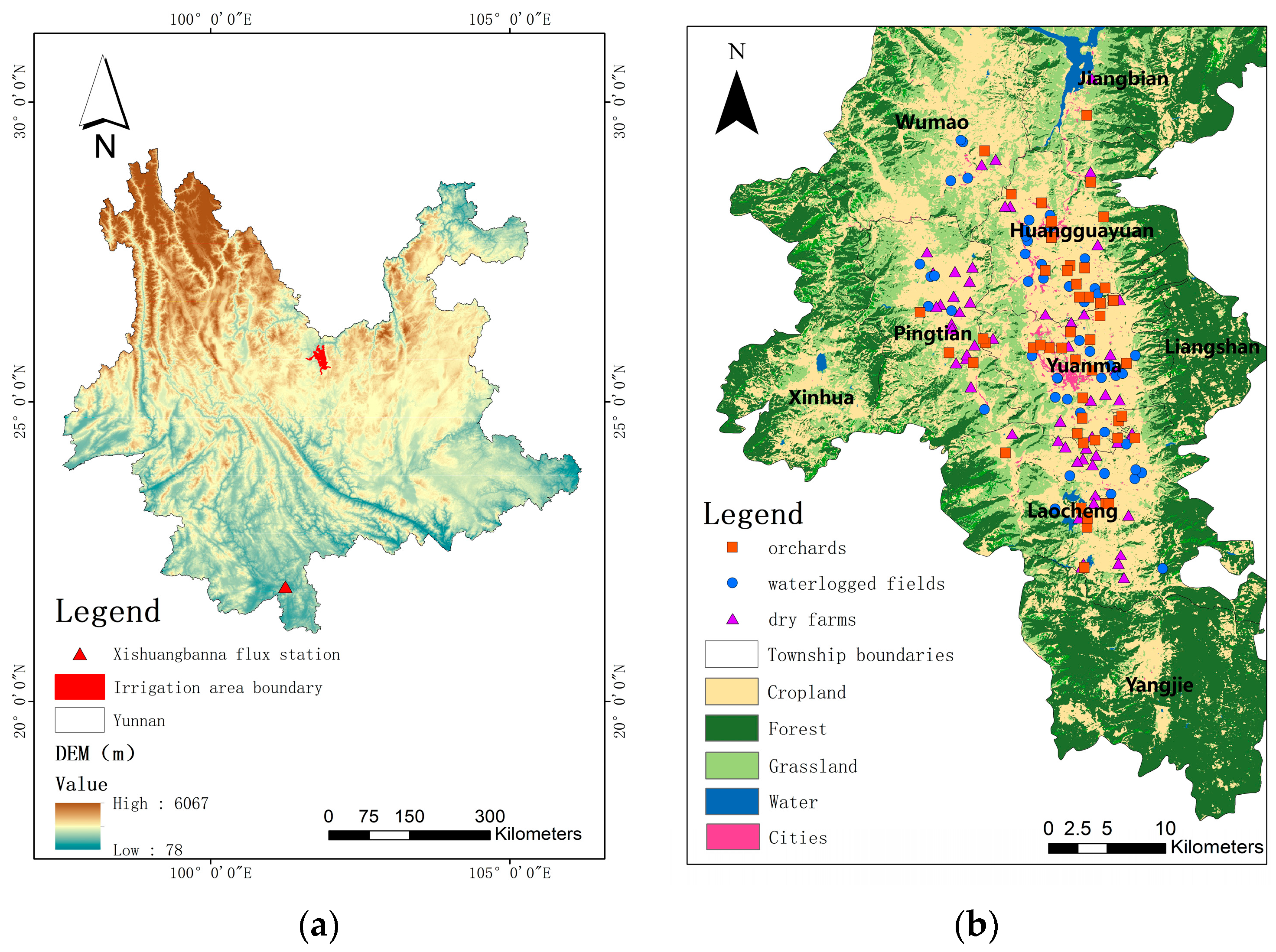
2.1. Study Area

This study focused on the Yuanmou Irrigation District as the research area (Figure 1). Located in Yuanmou County, Yunnan Province, the Yuanmou Irrigation District lies within the Jinsha River dry and hot valley region in the central Yunnan Plateau, characterized by a tropical climate. Regional soil types are predominantly loamy. The average annual rainfall is 642 mm, the average elevation is 1100 m, and the annual average temperature in the county is 21.9 °C, with extreme maximum temperatures reaching 43 °C. Benefiting from abundant solar radiation, suitable elevation, a hot climate, and the absence of a winter season throughout the year, it is often referred to as a “natural greenhouse.” This region is suitable for the growth of various plants and serves as a production base for developing tropical cash crops, early winter vegetables, and flowers.

The irrigation district covers seven townships in Yuanmou County, with a total population of 208,000. Major crops include rice, wheat, and corn, while economic crops mainly consist of vegetables, melons, and fruits. The water conservancy construction in the irrigation district adopts a combination of storage, diversion, and lifting methods, forming an irrigation system primarily based on headwater reservoirs and main trunk canals, supplemented by numerous water sources and canals under joint scheduling. The total land area of the irrigation district is 121,300 hm², with a cultivated area of 22,353 hm², a designed irrigation area of 21,333 hm², and an effective irrigated area of 20,600 hm².

2.2. Ground Monitoring Data

In this study, the meteorological data utilized were derived from climatic observation stations. These data encompassed variables such as temperature, pressure, relative humidity, precipitation, and wind speed. To achieve a spatial scale of 500 m, the station data were interpolated using the inverse distance weighting method. The land use data employed in this research were sourced from the “China 1985–2022 Annual Land Cover Dataset” released by Yang and Huang from Wuhan University (https://zenodo.org/records/8176941 (accessed on 1 February 2024)) [28]. Similarly, the land use data were resampled to a spatial scale of 500 m. These datasets were utilized for the estimation of ET using the Penman–Monteith–Leuning (PML) model. Furthermore, this study employed a combination of field surveys and visual interpretation to acquire 150 data points representing different types of cultivated land within the irrigation district. The cultivated land types included waterlogged fields, dry farms, and orchards. This study also utilized a dataset of carbon and water fluxes observed in the Xishuangbanna tropical seasonal rainforest from 2013 to 2015 (http://www.csdata.org/p/866/ (accessed on 14 March 2024)) [29] to validate the accuracy of ET inversion results and perform a sensitivity analysis of the parameters of PML model. The dataset was generated based on the Xishuangbanna Tropical Seasonal Rainforest Ecological Station (21°55′ N, 101°15′ E). This station is equipped with a flux tower, where an open-path eddy covariance flux system and a multi-layer micrometeorological observation system are installed for data monitoring purposes.

2.3. Remote Sensing Data

The computation of ET based on the PML model primarily relied on MODIS (https://www.earthdata.nasa.gov/ (accessed on 1 February 2024)) Leaf Area Index (LAI) data from the MCD15A2H product. The LAI product is a synthetic product with an 8-day temporal resolution and a spatial resolution of 500 m. Savitzky–Golay filtering interpolation was applied to obtain a daily data sequences. Radiation flux data from the ERA5 (https://cds.climate.copernicus.eu/cdsapp#!/home (accessed on 6 February 2024)) atmospheric reanalysis dataset were also utilized. This dataset includes surface net shortwave radiation and surface net longwave radiation, which are crucial for the calculation of ET. The spatial resolution of these flux data was 0.25°, and a third-order convolution interpolation method was employed to resample the data to a spatial resolution of 500 m. Sentinel-2 data (https://code.earthengine.google.com/ (accessed on 3 February 2024)) were used for bands 2, 3, 4, 8, and 11, primarily for calculating the normalized difference vegetation index (NDVI) and land surface water index (LSWI), which are essential for the downscaling calculation of ET. In addition to these datasets, MODIS ET data (MOD16A2) were employed for the accuracy assessment of the inverted ET results. This comprehensive approach involving multiple datasets contributed to a robust and accurate estimation of ET in the study area.

2.4. Methods

2.4.1. Penman–Monteith–Leuning Model

In this study, we employed the Penman–Monteith–Leuning (PML) model, which incorporates canopy retention evaporation [30] and distinguishes surface ET into three components: interception from vegetation canopy (E_i), soil evaporation (E_s), and vegetation transpiration (E_c). The primary equation used by the model is as follows [30,31,32]. The first term on the right represents the heat flux corresponding to E_i, the second term represents the heat flux corresponding to E_c, and the third term represents the heat flux corresponding to E_s:

$$\lambda E=F_i+\frac{\epsilon A_c+({\rho }_a{C}_p/\gamma )D_a{G}_a}{\epsilon +1+G_a/G_c}+\frac{f\epsilon A_s}{\epsilon +1}$$

(1)

in which $\lambda$ is the latent heat of the vaporization of water, MJ·kg⁻¹; $E$ is ET, mm·day⁻¹; $F_i$ is the heat flux corresponding to E_i, obtained by inverting the Penman–Monteith equation [33], MJ·m⁻²·day⁻¹; $\epsilon =s/\gamma$, where s is the slope of the temperature-saturated water pressure curve, kPa·°C⁻¹; $\gamma$ is the psychrometric constant, kPa·°C⁻¹; $A_c$ is the energy absorbed by the canopy, MJ·m⁻²·day⁻¹; ${\rho }_a$ is the density of the air, g·m⁻³; $C_p$ is the specific heat of the air at constant pressure, J·g⁻¹·°C⁻¹; $D_a$ is the vapor pressure deficit of the air, kPa; $G_a$ is the aerodynamic conductance, m·s⁻¹; $G_c$ is the canopy conductance, m·s⁻¹; $f$ is the soil evaporation coefficient, which is set as 0.6; and $A_s$ is the energy absorbed by the soil, MJ·m⁻²·day⁻¹.

This study enhanced the PML model using the vegetation canopy interception model developed by Duan et al. [32] to compute E_i. This model represents canopy interception as a function of LAI, with the calculation method as follows:

$$E_i=S_{max}\left[1-e^{-0.04LAI\frac{P_{cum}}{S_{max}}}\right]$$

(2)

where $S_{max}$ is the retention capacity, mm·day⁻¹; $LAI$ is the leaf area index, m²·m⁻²; and $P_{cum}$ is the daily precipitation, mm·day⁻¹.

2.4.2. ET Downscales

In order to enhance the accuracy of ET inversion results at the field scale, this study employed the ET downscaling method proposed by Ma et al. [27]. The crop growth conditions and field moisture, correlated with crop transpiration capacity based on stomatal behavior and soil moisture status, collectively influence on-field ET. In our investigation, we disregarded the potential horizontal vapor transport from adjacent fields. Based on the two classes of virtually unchanged and field-variant parameters that influenced ET, the ET capacity of each field could be evaluated. Thus, we could assume that, between adjacent fields within a coarse ET pixel, some allocation factors derived from the field-variant parameters could be regarded as equivalent to the ET capacity of each field. The relation above can be summarized using the following equation [27]:

$${\mathrm{E}\mathrm{T}}_{{\mathrm{f}\mathrm{i}\mathrm{e}\mathrm{l}\mathrm{d}}_1}:{\mathrm{E}\mathrm{T}}_{{\mathrm{f}\mathrm{i}\mathrm{e}\mathrm{l}\mathrm{d}}_2}:\cdots {\mathrm{E}\mathrm{T}}_{{\mathrm{f}\mathrm{i}\mathrm{e}\mathrm{l}\mathrm{d}}_i}=A{F}_{fiel{d}_1}:A{F}_{fiel{d}_2}:\cdots A{F}_{fiel{d}_i}$$

(3)

where ${\mathrm{E}\mathrm{T}}_{{\mathrm{f}\mathrm{i}\mathrm{e}\mathrm{l}\mathrm{d}}_i}$ represents the ET of the ith field (i = 1, 2, ··· n) within each coarse ET pixel and $A{F}_{fiel{d}_i}$ represents the allocation factor of the field i (i = 1, 2, ··· n) within each coarse ET pixel. Additionally, the relationship between the ET of field i and the coarse ET pixel can be expressed as follows [27]:

$$\frac{{\mathrm{E}\mathrm{T}}_{{\mathrm{f}\mathrm{i}\mathrm{e}\mathrm{l}\mathrm{d}}_i}}{{\mathrm{E}\mathrm{T}}_{\mathrm{c}\mathrm{o}\mathrm{a}\mathrm{r}\mathrm{s}\mathrm{e}}}=\frac{A{F}_{fiel{d}_i}}{A{F}_{\mathrm{c}\mathrm{o}\mathrm{a}\mathrm{r}\mathrm{s}\mathrm{e}}}$$

(4)

where $A{F}_{\mathrm{c}\mathrm{o}\mathrm{a}\mathrm{r}\mathrm{s}\mathrm{e}}$ represents the mean allocation factor of the coarse pixel and ${\mathrm{E}\mathrm{T}}_{\mathrm{c}\mathrm{o}\mathrm{a}\mathrm{r}\mathrm{s}\mathrm{e}}$ represents the ET value of a coarse resolution pixel. With Equation (4), each field ET within the coarse ET pixel can be calculated based on the allocation factor, which can also be regarded as the allocation of the coarse pixel-level (500 m level) ET to the farm-level (10 m level) ET.

The following section describes how the field allocation factor was derived. The Priestley–Taylor (PT) equation is suitable for estimating ET under ample soil moisture conditions [34,35], such as in irrigated agricultural fields. The PT equation is independent of surface resistance and aerodynamic resistance and is calculated based on meteorological data and the coefficient α. The PT equation was primarily developed to estimate potential evaporation, but, for practical ET applications, the α coefficient should be adjusted using several constraint functions, such as surface moisture, temperature, and the fraction of absorbed photosynthetically active radiation (fapar) [35]. Here, we used the vegetation cover fraction (FVC) to represent the upper limit of fapar, as done in several studies [36]. We employed the remotely sensed land surface water index (LSWI) as a constraint for soil water. LSWI is a normalized index based on the near-infrared (NIR) and short-wave infrared (SWIR) bands [37,38,39].

The PT equation can be expressed as follows [27]:

$$LE=f(lswi,fvc,t)\alpha \frac{\mathsf{\Delta }}{\mathsf{\Delta }+\gamma }(R_n-G)$$

(5)

where the coefficient α in the PT equation is initially set to 1.26 and Δ and γ are the same as in the PM equation. f(lswi) represents the surface moisture constraint, where low surface moisture conditions limit the volume of ET. f(t) represents the temperature constraint, with the optimal temperature for transpiration being the most suitable temperature for the process. f(fvc) represents the radiation constraint, where lower FVC limits the net radiation in the transpiration process.

When focusing on agricultural fields, crop transpiration is a major component of ET. Ma et al. [27] proposed the assumption that daily environmental conditions (temperature, relative humidity, wind speed, and net radiation) remain relatively constant at the field scale within coarse pixels. Based on this assumption, certain parts of the PT equation can be neglected at the field scale: Δ and γ are calculated based on relative humidity and air temperature, while Rn is mainly influenced by solar shortwave radiation, which is calculated based on sunshine duration and longwave radiation from the surface emissivity and air temperature. These meteorological components can be neglected because the vegetation types in agricultural fields are uniform and the differences in emissivity between fields are minimal. We disregarded the Rn portion of the field allocation factor, and G could be regarded as a constant part of Rn [40]; thus, G was also neglected. Based on these assumptions, a method was derived to calculate the field allocation factor using the ET constraint functions.

The field allocation factor calculation equation was as follows [27]:

$$A{F}_{fiel{d}_i}=1-max\left(min\left(\frac{FV{C}_{max}-FVC}{FV{C}_{max}-FV{C}_{min}},1\right),0\right)·max\left(min\left(\frac{LSW{I}_{max}-LSWI}{LSW{I}_{max}-LSW{I}_{min}},1\right),0\right)$$

(6)

where FVC indicates the vegetation cover fraction, LSWI indicates the land surface water index, LSWI_max indicates the high moisture condition, LSWI_min indicates the dry condition, and the FVC_max is set as 0.95.

2.4.3. Irrigation Area Identification Based on ET

Analyses of water in agricultural regions from a water balance perspective reveal that field-supplied water primarily consists of the irrigation and effective precipitation of ET. The predominant water consumption in agricultural areas is attributed to field ET, with the crop’s inherent moisture content deemed negligible. Therefore, ET can be deconstructed in terms of volume into two components: ET induced by irrigation and ET triggered by effective precipitation. The extent of irrigation is discernible within the overall ET volume.

Through water balance analysis of irrigation districts, field ET can be further decomposed into ET from precipitation and ET from irrigation. By deducting the impact of precipitation of ET through the computation of effective precipitation, the residual change in ET is attributed to irrigation-induced effective ET [23]:

$$ET=P\_eff+ET\_eff$$

(7)

where ET can be retrieved through remote sensing data, while effective precipitation ($P\_eff$) can be calculated using a specific formula. The difference between these two values yields the variation in ET induced by irrigation ($ET\_eff$).

In rainfed agriculture, effective precipitation is defined as the amount of precipitation consumed in the ET process during crop growth. In agricultural research, the portion of precipitation that forms surface runoff and infiltration is considered ineffective precipitation. We used a method commonly recommended by the U.S. Department of Agriculture Soil Conservation and the FAO CROPWAT model to calculate $P\_eff$. This method operates on a daily calculation basis. The specific formula is as follows [40,41]:

$$P\_eff=\left\{\begin{array}{c}\frac{P(4.17-0.2P)}{4.17},P<8.3 \mathrm{mm}/\mathrm{d}\\ 4.17+0.1P,P\ge 8.3 \mathrm{mm}/\mathrm{d}\end{array}\right.$$

(8)

where P represents daily precipitation in millimeters (mm).

Irrigation increases ET, but such increments are challenging to discern on a daily scale due to the multifaceted influences on ET, including meteorological elements and radiation. There are significant daily-scale fluctuations. However, over longer time scales, the impact of irrigation on crop ET becomes more apparent [22]. By calculating the effective ET, this study investigates the response of ET to agricultural irrigation at an annual scale, appropriate threshold values can typically be selected to identify the actual irrigated area for a given year.

3. Results and Discussion

3.1. Evaluation of ET Inversion Accuracy

Currently, the methods for evaluating the accuracy of ET inversion mainly include direct verification and indirect verification. The direct verification method is based on the surface ET relative true value at pixel or regional scales to verify surface ET remote sensing products. The relative true value is obtained based on observed data. In the absence of pixel- or regional-scale relative true values, the cross-validation method and the indirect verification method can be used. The cross-validation method can be applied when there are no ground observation data for surface ET in the verification area but there are already verified surface ET products.

This study first evaluated the accuracy of ET inversion using the 2013–2015 tropical seasonal rainforest carbon flux observation dataset of Xishuangbanna. Simultaneously, the sensitivity of the soil evaporation coefficient, as an important parameter in the model, on the accuracy of ET inversion was assessed. Here, we tested the sensitivity of the soil evaporation coefficient within the range of 0.5–0.8, with a step size of 0.1. The results are shown in Figure 2. The results indicate that within this range, the soil evaporation coefficient has a minor influence on the accuracy of ET inversion, with R² values consistently above 0.57. Among the tested values, the highest R² value of 0.59 was achieved when the soil evaporation coefficient was set to 0.6. Therefore, in this study, the soil evaporation coefficient was set as 0.6 for model calculations.

Due to the lack of ET data observation equipment in the study area, a cross-validation method was used to further indirectly assess the accuracy of ET inversion, and the ET product used was MODIS ET product MOD16. In order to comprehensively compare the accuracy of ET inversion results in terms of temporal and spatial scales, this study selected typical representative points on different types of farmland (waterlogged fields, dry farms, orchards) and evaluated the comparison between the ET inversion results and MOD16 for the whole year at each representative point, as shown in Figure 3. Through the analysis, it was found that the fitting results of the ET inversion results and MOD16 were good, with R² values of the three different types of farmland all above 0.7, indicating a high correlation. Among them, the fitting accuracy of the PML model’s ET inversion results for paddy fields and orchards was better than that for dry fields, with R² values above 0.8. In terms of the annual process, the change trend of the PML model’s ET inversion results was more consistent with MOD16, and the correlation in summer was better than that in winter, with the ET inversion results of the PML model in winter lower than those of MOD16. In addition, comparing the ET values of the three different types of farmland, it was found that the annual ET total of paddy fields and orchards was higher than that of dry fields, indicating that the total annual ET was affected by irrigation.

3.2. Downscaling Calculation of ET and Spatial Distribution of Annual Cumulative Effective ET

3.2.1. Downscaling Calculation of ET

To enhance the identification accuracy of actual irrigated areas within the irrigation district, we employed the ET downscaling method proposed by Ma et al. [27] to further downscale the ET retrieval results of the PML model. The investigation into ET influencing factors at the parcel scale revealed that ET was primarily influenced by meteorological conditions, such as atmospheric temperature and the saturation vapor pressure deficit. Differences in vegetation coverage affected surface net radiation, while variations in soil moisture led to differences in ET water supply. At the parcel scale, meteorological differences were relatively small. The main impacts on ET arose from surface crop growth and differences in soil moisture. Based on the concept of parcel-scale ET, this study focused on factors contributing to ET variations at the parcel scale. It calculated ET “allocation factors” [27] that measured water consumption differences between parcels and combined them with low-to-medium-resolution ET data to distribute ET at the parcel scale.

However, downsizing within a coarse-resolution pixel based on the overall and internal high-resolution pixel distribution relationship resulted in the “edge effect”. The bordering sections of adjacent coarse pixels were retained in the high-resolution result, introducing spatial result uncertainty. Therefore, prior to downsizing, a three-time convolution method was applied to smooth the 500 m scale ET inversion results, eliminating the “edge effect”. The final downscaled ET results are presented in Figure 4.

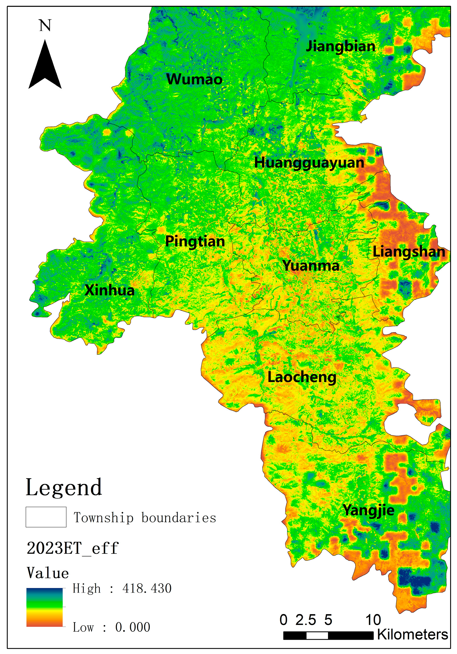
3.2.2. Spatial Distribution Characteristics of Cumulative Effective ET in 2023

Following the methodology outlined in Section 2.4.3, the cumulative annual effective ET for the study area in 2023 was computed based on the ET downscaled calculations mentioned in the preceding research. Concurrently, the effective rainfall for the study area in 2023 was calculated on an annual scale using precipitation data and Equation (8), likewise accumulated annually. Subsequently, the annual total of effective ET was obtained by subtracting the annual total of effective rainfall from the annual total of ET, as illustrated in Figure 5.

The annual total of effective ET reflected the frequency and magnitude of irrigation events and irrigation water volume in the study area in 2023. A higher annual total of effective ET indicated a greater frequency of irrigation events and a larger irrigation water volume for the year, while a lower total suggested fewer irrigation events and a smaller irrigation water volume in the area. As depicted in the figure, the annual total of effective ET in the study area in 2023 exhibited a spatial pattern of higher values in the northern region and lower values in the southern region. This distribution pattern may be attributed to the spatial characteristics of annual precipitation in the study area in 2023, where the southern region received higher annual precipitation compared to the northern region, resulting in fewer irrigation events and a lower irrigation water volume in the southern region of the study area.

3.3. Irrigation Area Identification Based on Cumulative Effective ET

Based on field surveys and visual interpretation of sample points, out of 150 recorded points, 50 were identified as non-irrigated locations. Extracting the corresponding annual total of effective ET for the year 2023 from these points, the maximum value among them was determined to be the threshold for determining the irrigation area in the study region, set as 87 mm. Thus, areas with an annual total of effective ET greater than 87 mm in 2023 were considered as experiencing irrigation. Furthermore, it was necessary to exclude areas outside the study region and regions classified as non-agricultural land use types.

Based on the extraction method proposed in this study, the actual irrigated area of the region can be extracted. The resulting map of the distribution of irrigated areas in the study area for the year 2023 is shown in Figure 6. The total irrigated area interpreted from remote sensing data for the study area in 2023 is approximately 15,000 hm². Verification was conducted using sample point data from the study area, with 100 sample points identified as irrigated locations. Upon comparing these irrigated sample points with the remotely sensed interpreted irrigated areas, 84 sample points were correctly extracted, resulting in an extraction error of 16%, which is relatively small.

3.4. Uncertainties and Limitations of This Study

This study employed the PML model inversion and ET downscale methods to estimate ET at a 10 m scale and investigated the identification of annual irrigated areas by calculating the effective ET. However, these methods entailed some uncertainties arising from parameter estimation, model assumptions, and data inputs. In this section, we aim to elucidate the uncertainties associated with each method and propose strategies to address or mitigate these uncertainties.

Firstly, the PML model is characterized by a high degree of complexity, involving numerous variables and equations for estimating ET components. Simplifications or assumptions made during model construction may introduce uncertainty. From the perspective of data input, since fine field meteorological data are not easily available, this study performed ET inversion by interpolating the data from meteorological stations, which can introduce uncertainty in ET simulation. Subsequent efforts are needed to improve the spatial and temporal accuracy of meteorological data.

There was also uncertainty in the analysis of ET due to irrigation. Firstly, the calculation of effective precipitation relied on empirical relationships. However, the accuracy of the rainfall monitoring data and the local applicability of the effective rainfall methodology adopted in this paper will have impacted the results of the effective rainfall analysis. Secondly, the definition of thresholds used for identifying irrigated areas relied on empirical analysis and spatial pattern recognition. However, uncertainties in threshold definition were influenced by factors such as data quality, spatial heterogeneity, and dynamics of the cropping structure, all of which need to be optimally adjusted in subsequent threshold analyses.

4. Conclusions

This study employed remote sensing-based ET inversion and downscaling calculations to achieve an actual irrigated area identification method at an annual temporal scale. The key findings of this approach are summarized as follows:

(1)

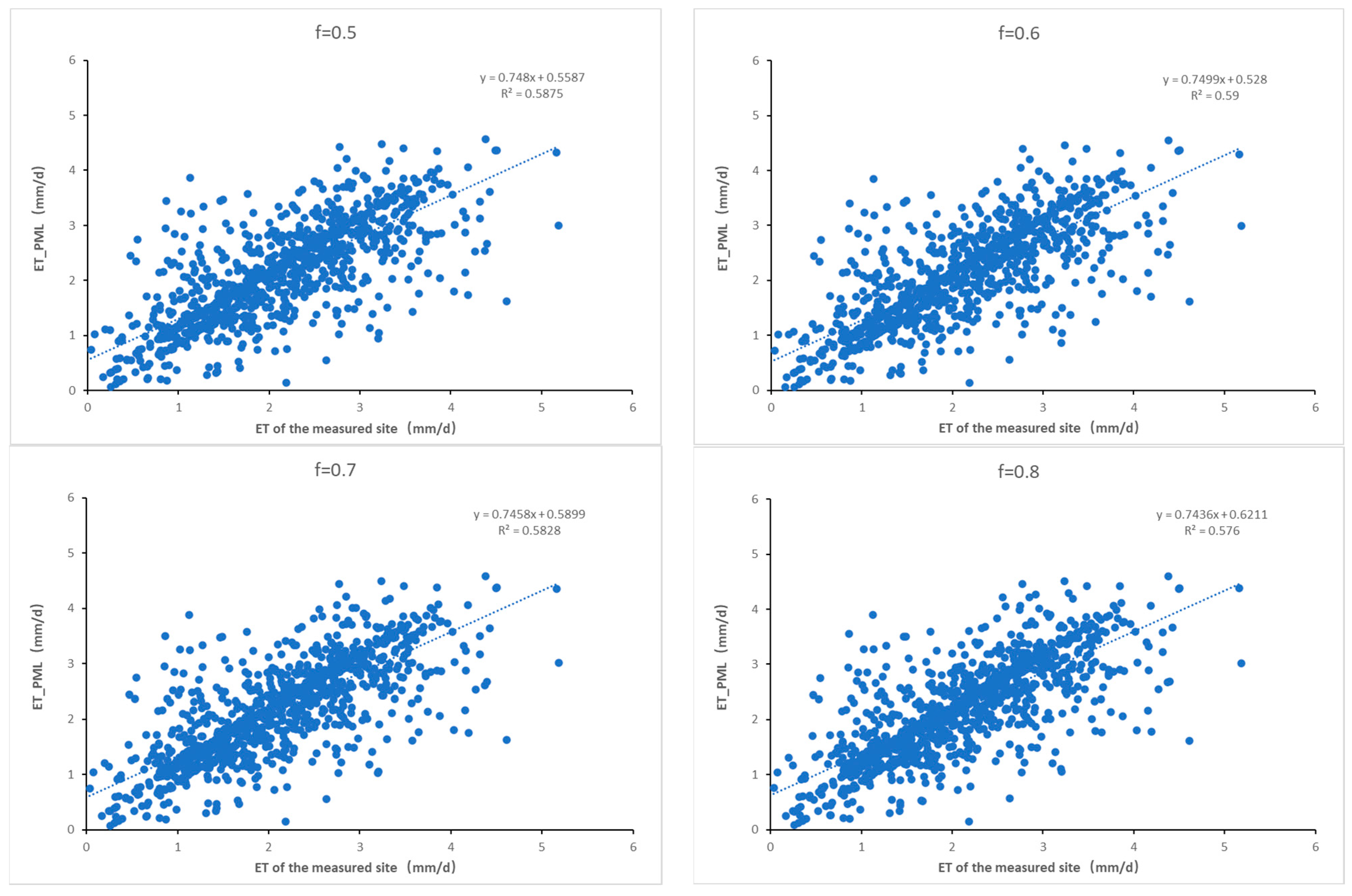
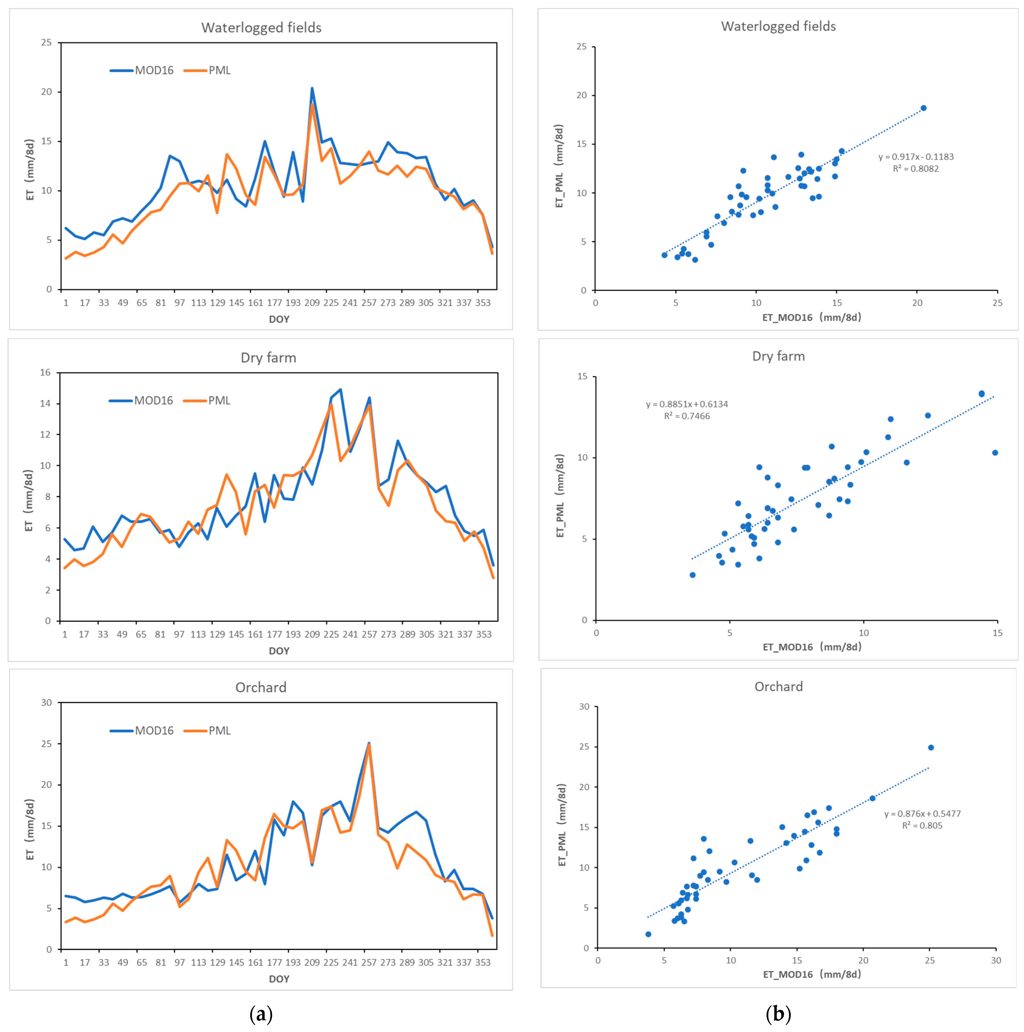
Evaluation of ET Inversion Accuracy: The evaluation of ET inversion accuracy revealed promising results. The R² between the simulation results of ET in this paper and the measured data of Xishuangbanna station was 0.59, which was in good agreement. The ET obtained in this paper was also in good agreement with the MODIS ET product, particularly evident in the fitting accuracy across different types of farmland. The R² obtained, exceeding 0.7 for all land types and surpassing 0.8 for paddy fields and orchards, underscores the reliability of the PML model in capturing ET variations.

(2)

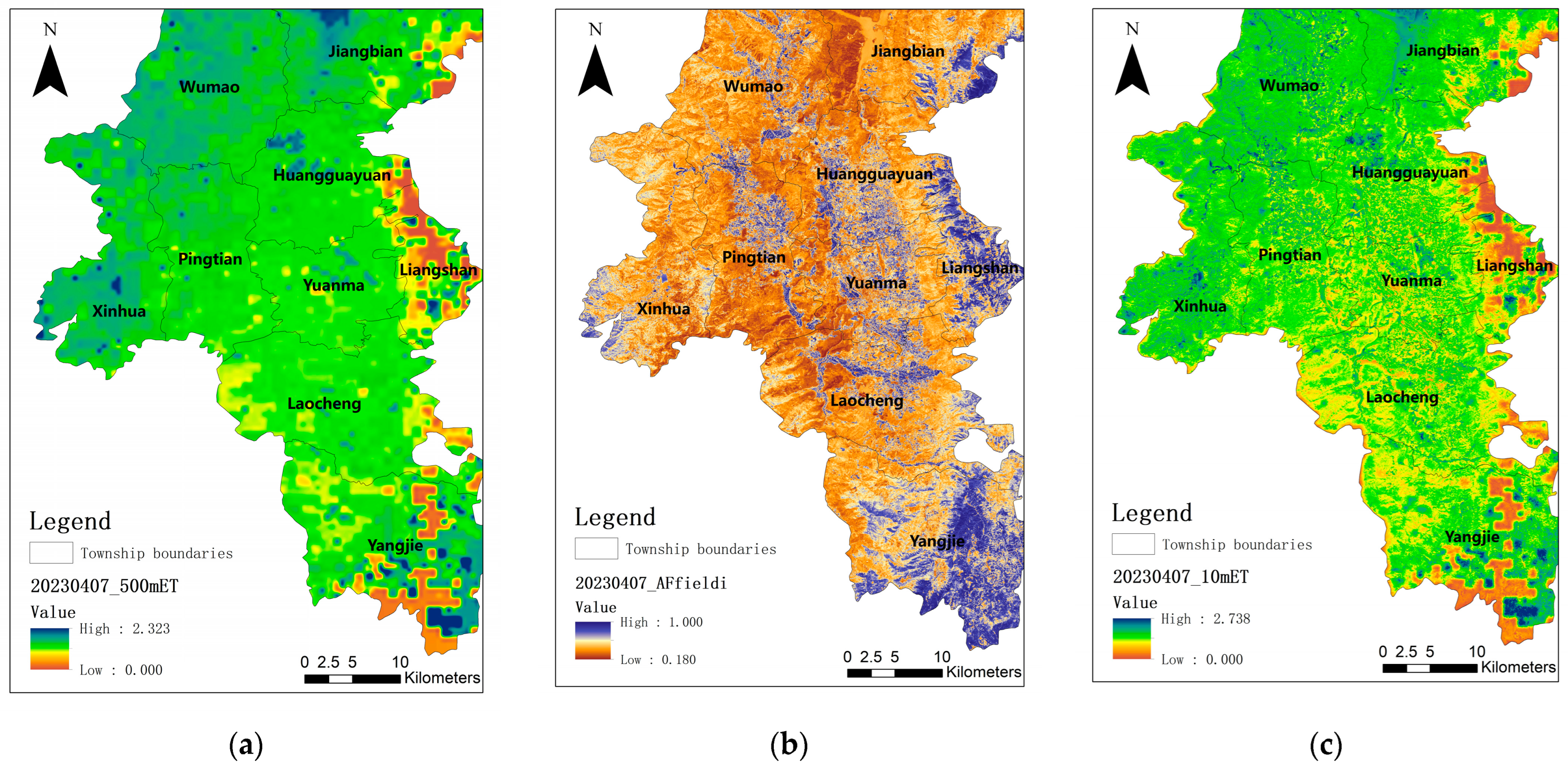
Downscaling of ET: To address the limitations posed by coarse spatial resolution, a downscaling approach was implemented, enhancing the accuracy of ET estimation at the parcel scale. By considering factors influencing ET variations at the parcel level, such as meteorological conditions and surface characteristics, this study successfully distributed ET at a finer spatial resolution of 10 m.

(3)

Spatial Distribution Characteristics of Cumulative Effective ET: The spatial distribution of cumulative effective ET in 2023 elucidated distinct patterns influenced by regional climatic factors and agricultural practices. The observed higher values in the northern region compared to the southern region corresponded with precipitation patterns, indicating a correlation between effective ET and regional climate conditions.

(4)

Irrigation Area Identification: Leveraging remote sensing data, this study identified irrigated areas based on cumulative effective ET, achieving a close approximation to actual recorded data with a small margin of error. The interpretation of remote sensing data proved effective in delineating irrigated areas, highlighting its utility in agricultural water resource management.

Despite the valuable insights gained from this research, it is essential to acknowledge the inherent limitations inherent in the methodologies employed. Challenges related to model parameter accuracy, data scale conversion, and uncertainties in remote sensing-derived ET estimation underscore the need for the ongoing refinement and validation of methodologies. Efforts to address these limitations are crucial to improve the accuracy and reliability of ET estimation and irrigation area identification and to promote agricultural water management capacity.

References

1. Leakey, A.D.B.; Ferguson, J.N.; Pignon, C.P.; Wu, A.; Jin, Z.; Hammer, G.L.; Lobell, D.B. Water Use Efficiency as a Constraint and Target for Improving the Resilience and Productivity of C3 and C4 Crops. Annu. Rev. Plant Biol. 2019, 70, 781–808. [Google Scholar] [CrossRef]
2. Elliott, J.; Deryng, D.; Müller, C.; Frieler, K.; Konzmann, M.; Gerten, D.; Glotter, M.; Flörke, M.; Wada, Y.; Best, N.; et al. Constraints and Potentials of Future Irrigation Water Availability on Agricultural Production under Climate Change. Proc. Natl. Acad. Sci. USA 2014, 111, 3239–3244. [Google Scholar] [CrossRef]
3. China Water Resources Bulletin Ministry of Water Resources of the People’s Republic of China. 2020. Available online: http://www.mwr.gov.cn/sj/tjgb/szygb/202107/t20210709_1528208.html (accessed on 3 February 2024).
4. Liu, M.; Yang, L.; Min, Q. Water-Saving Irrigation Subsidy Could Increase Regional Water Consumption. J. Clean. Prod. 2019, 213, 283–288. [Google Scholar] [CrossRef]
5. Chen, F.; Zhao, H.; Roberts, D.; Van De Voorde, T.; Batelaan, O.; Fan, T.; Xu, W. Mapping Center Pivot Irrigation Systems in Global Arid Regions Using Instance Segmentation and Analyzing Their Spatial Relationship with Freshwater Resources. Remote Sens. Environ. 2023, 297, 113760. [Google Scholar] [CrossRef]
6. Ozdogan, M.; Gutman, G. A New Methodology to Map Irrigated Areas Using Multi-Temporal MODIS and Ancillary Data: An Application Example in the Continental US. Remote Sens. Environ. 2008, 112, 3520–3537. [Google Scholar] [CrossRef]
7. Zhang, C.; Dong, J.; Ge, Q. Mapping 20 Years of Irrigated Croplands in China Using MODIS and Statistics and Existing Irrigation Products. Sci. Data 2022, 9, 407. [Google Scholar] [CrossRef]
8. Potapov, P.; Turubanova, S.; Hansen, M.C.; Tyukavina, A.; Zalles, V.; Khan, A.; Song, X.-P.; Pickens, A.; Shen, Q.; Cortez, J. Global Maps of Cropland Extent and Change Show Accelerated Cropland Expansion in the Twenty-First Century. Nat. Food 2021, 3, 19–28. [Google Scholar] [CrossRef]
9. Massari, C.; Modanesi, S.; Dari, J.; Gruber, A.; De Lannoy, G.J.M.; Girotto, M.; Quintana-Seguí, P.; Le Page, M.; Jarlan, L.; Zribi, M.; et al. A Review of Irrigation Information Retrievals from Space and Their Utility for Users. Remote Sens. 2021, 13, 4112. [Google Scholar] [CrossRef]
10. Velpuri, N.M.; Thenkabail, P.S.; Gumma, M.K.; Biradar, C.; Dheeravath, V.; Noojipady, P.; Yuanjie, L. Influence of Resolution in Irrigated Area Mapping and Area Estimation. Photogramm. Eng. Remote Sens. 2009, 75, 1383–1395. [Google Scholar] [CrossRef]
11. Ambika, A.K.; Wardlow, B.; Mishra, V. Remotely Sensed High Resolution Irrigated Area Mapping in India for 2000 to 2015. Sci. Data 2016, 3, 160118. [Google Scholar] [CrossRef]
12. Yao, Z.; Cui, Y.; Geng, X.; Chen, X.; Li, S. Mapping Irrigated Area at Field Scale Based on the OPtical TRApezoid Model (OPTRAM) Using Landsat Images and Google Earth Engine. IEEE Trans. Geosci. Remote Sens. 2022, 60, 4409011. [Google Scholar] [CrossRef]
13. Dari, J.; Quintana-Seguí, P.; Escorihuela, M.J.; Stefan, V.; Brocca, L.; Morbidelli, R. Detecting and Mapping Irrigated Areas in a Mediterranean Environment by Using Remote Sensing Soil Moisture and a Land Surface Model. J. Hydrol. 2021, 596, 126129. [Google Scholar] [CrossRef]
14. Gao, Q.; Zribi, M.; Escorihuela, M.; Baghdadi, N.; Segui, P. Irrigation Mapping Using Sentinel-1 Time Series at Field Scale. Remote Sens. 2018, 10, 1495. [Google Scholar] [CrossRef]
15. Zohaib, M.; Choi, M. Satellite-Based Global-Scale Irrigation Water Use and Its Contemporary Trends. Sci. Total Environ. 2020, 714, 136719. [Google Scholar] [CrossRef]
16. Zaussinger, F.; Dorigo, W.; Gruber, A.; Tarpanelli, A.; Filippucci, P.; Brocca, L. Estimating Irrigation Water Use over the Contiguous United States by Combining Satellite and Reanalysis Soil Moisture Data. Hydrol. Earth Syst. Sci. 2019, 23, 897–923. [Google Scholar] [CrossRef]
17. Zhang, Y.; Li, X. Analyses of Supply-Demand Balance of Agricultural Products in China and Its Policy Implication. J. Nat. Resour. 2021, 36, 1573. [Google Scholar] [CrossRef]
18. Katul, G.G.; Oren, R.; Manzoni, S.; Higgins, C.; Parlange, M.B. Evapotranspiration: A Process Driving Mass Transport and Energy Exchange in the Soil-plant-atmosphere-climate System. Rev. Geophys. 2012, 50, 2011RG000366. [Google Scholar] [CrossRef]
19. Merlin, O.; Chirouze, J.; Olioso, A.; Jarlan, L.; Chehbouni, G.; Boulet, G. An Image-Based Four-Source Surface Energy Balance Model to Estimate Crop Evapotranspiration from Solar Reflectance/Thermal Emission Data (SEB-4S). Agric. For. Meteorol. 2014, 184, 188–203. [Google Scholar] [CrossRef]
20. Idso, S.B.; Jackson, R.D.; Reginato, R.J. Estimating Evaporation: A Technique Adaptable to Remote Sensing. Science 1975, 189, 991–992. [Google Scholar] [CrossRef]
21. Jensen, M.E.; Haise, H.R. Estimating Evapotranspiration from Solar Radiation. J. Irrig. and Drain. Div. 1963, 89, 15–41. [Google Scholar] [CrossRef]
22. Geli, H.M.E.; González-Piqueras, J.; Neale, C.M.U.; Balbontín, C.; Campos, I.; Calera, A. Effects of Surface Heterogeneity Due to Drip Irrigation on Scintillometer Estimates of Sensible, Latent Heat Fluxes and Evapotranspiration over Vineyards. Water 2019, 12, 81. [Google Scholar] [CrossRef]
23. Li, X.; Zhang, Y.; Ma, N.; Zhang, X.; Tian, J.; Zhang, L.; McVicar, T.R.; Wang, E.; Xu, J. Increased Grain Crop Production Intensifies the Water Crisis in Northern China. Earth’s Future 2023, 11, e2023EF003608. [Google Scholar] [CrossRef]
24. Chemin, Y.; Platonov, A.; Ul-Hassan, M.; Abdullaev, I. Using Remote Sensing Data for Water Depletion Assessment at Administrative and Irrigation-System Levels: Case Study of the Ferghana Province of Uzbekistan. Agric. Water Manag. 2004, 64, 183–196. [Google Scholar] [CrossRef]
25. Allen, R.G.; Tasumi, M.; Morse, A.; Trezza, R. A Landsat-Based Energy Balance and Evapotranspiration Model in Western US Water Rights Regulation and Planning. Irrig. Drain. Syst. 2005, 19, 251–268. [Google Scholar] [CrossRef]
26. Alexandridis, T.K.; Panagopoulos, A.; Galanis, G.; Alexiou, I.; Cherif, I.; Chemin, Y.; Stavrinos, E.; Bilas, G.; Zalidis, G.C. Combining Remotely Sensed Surface Energy Fluxes and GIS Analysis of Groundwater Parameters for Irrigation System Assessment. Irrig. Sci. 2014, 32, 127–140. [Google Scholar] [CrossRef]
27. Ma, Z.; Wu, B.; Yan, N.; Zhu, W.; Zeng, H.; Xu, J. Spatial Allocation Method from Coarse Evapotranspiration Data to Agricultural Fields by Quantifying Variations in Crop Cover and Soil Moisture. Remote Sens. 2021, 13, 343. [Google Scholar] [CrossRef]
28. Yang, J.; Huang, X. The 30 m Annual Land Cover Datasets and Its Dynamics in China from 1985 to 2022. 2023. [Google Scholar] [CrossRef]
29. Liu, Y.; Zhang, J.; Zheng, H.; Fei, X.; Sha, L.; Zhou, W.; Zhou, L.; Deng, X.; Luo, Y.; Deng, Y.; et al. A Dataset of Carbon and Water Fluxes Observed in Xishuangbanna Tropical Seasonal Rain Forest from 2011 to 2015. 2023, 23617225 bytes, 1 files. 2023, 8. [Google Scholar] [CrossRef]
30. Leuning, R.; Zhang, Y.Q.; Rajaud, A.; Cleugh, H.; Tu, K. A Simple Surface Conductance Model to Estimate Regional Evaporation Using MODIS Leaf Area Index and the Penman-Monteith Equation. Water Resour. Res. 2008, 44, 2007WR006562. [Google Scholar] [CrossRef]
31. Leuning, R. A Critical Appraisal of a Combined Stomatal-photosynthesis Model for C3 Plants. Plant Cell Environ. 1995, 18, 339–355. [Google Scholar] [CrossRef]
32. Duan, H.; Lu, S. The Inffuence of Canopy Interception on Evapotranspiration and Energy Distribution of PML Model. China Rural. Water Hydropower 2021, 9, 80–84. [Google Scholar]
33. Zheng, C.; Jia, L.; Hu, G.; Lu, J. Earth Observations-Based Evapotranspiration in Northeastern Thailand. Remote Sens. 2019, 11, 138. [Google Scholar] [CrossRef]
34. Hao, Y.; Baik, J.; Choi, M. Developing a Soil Water Index-Based Priestley–Taylor Algorithm for Estimating Evapotranspiration over East Asia and Australia. Agric. For. Meteorol. 2019, 279, 107760. [Google Scholar] [CrossRef]
35. Fisher, J.B.; Tu, K.P.; Baldocchi, D.D. Global Estimates of the Land–Atmosphere Water Flux Based on Monthly AVHRR and ISLSCP-II Data, Validated at 16 FLUXNET Sites. Remote Sens. Environ. 2008, 112, 901–919. [Google Scholar] [CrossRef]
36. Zhang, Y.; Kong, D.; Gan, R.; Chiew, F.H.S.; McVicar, T.R.; Zhang, Q.; Yang, Y. Coupled Estimation of 500 m and 8-Day Resolution Global Evapotranspiration and Gross Primary Production in 2002–2017. Remote Sens. Environ. 2019, 222, 165–182. [Google Scholar] [CrossRef]
37. Chandrasekar, K.; Sesha Sai, M.V.R.; Roy, P.S.; Dwevedi, R.S. Land Surface Water Index (LSWI) Response to Rainfall and NDVI Using the MODIS Vegetation Index Product. Int. J. Remote Sens. 2010, 31, 3987–4005. [Google Scholar] [CrossRef]
38. Xiao, X.; Zhang, Q.; Saleska, S.; Hutyra, L.; De Camargo, P.; Wofsy, S.; Frolking, S.; Boles, S.; Keller, M.; Moore, B. Satellite-Based Modeling of Gross Primary Production in a Seasonally Moist Tropical Evergreen Forest. Remote Sens. Environ. 2005, 94, 105–122. [Google Scholar] [CrossRef]
39. Zheng, Y.; Zhang, M.; Zhang, X.; Zeng, H.; Wu, B. Mapping Winter Wheat Biomass and Yield Using Time Series Data Blended from PROBA-V 100- and 300-m S1 Products. Remote Sens. 2016, 8, 824. [Google Scholar] [CrossRef]
40. Cao, X.; Zeng, W.; Wu, M.; Guo, X.; Wang, W. Hybrid Analytical Framework for Regional Agricultural Water Resource Utilization and Efficiency Evaluation. Agric. Water Manag. 2020, 231, 106027. [Google Scholar] [CrossRef]
41. Döll, P.; Siebert, S. Global Modeling of Irrigation Water Requirements. Water Resour. Res. 2002, 38, 8-1–8-10. [Google Scholar] [CrossRef]
Figure 1. Overview of the study area. (a) Location of the Yuanmou Irrigation District in Yunnan Province, China. (b) Distribution of measured points in Yuanmou Irrigation District.
Atmosphere 15 00492 g001
Figure 2. Sensitivity of soil evaporation coefficient in the interval of 0.5–0.8.
Atmosphere 15 00492 g002
Figure 3. Precision assessment of ET inversion in PML model. (a) Temporal variations of ET at various representative points. (b) Scatter plot comparisons of ET inversion results in PML model and MOD16 product at different representative points.
Atmosphere 15 00492 g003
Figure 4. (a) The inversion results of ET at a spatial resolution of 500 m. (b) The ET allocation factors. (c) The downscaled ET outcomes at a finer spatial resolution of 10 m.
Atmosphere 15 00492 g004
Figure 5. The annual cumulative value of effective ET.
Atmosphere 15 00492 g005
Figure 6. Irrigation map interpreted by remote sensing in the study area in 2023.
Atmosphere 15 00492 g006
Disclaimer/Publisher’s Note: The statements, opinions and data contained in all publications are solely those of the individual author(s) and contributor(s) and not of MDPI and/or the editor(s). MDPI and/or the editor(s) disclaim responsibility for any injury to people or property resulting from any ideas, methods, instructions or products referred to in the content.