
Contribution of Atmospheric Factors in Predicting Sea Surface Temperature in the East China Sea Using the Random Forest and SA-ConvLSTM Model


Abstract
1. Introduction
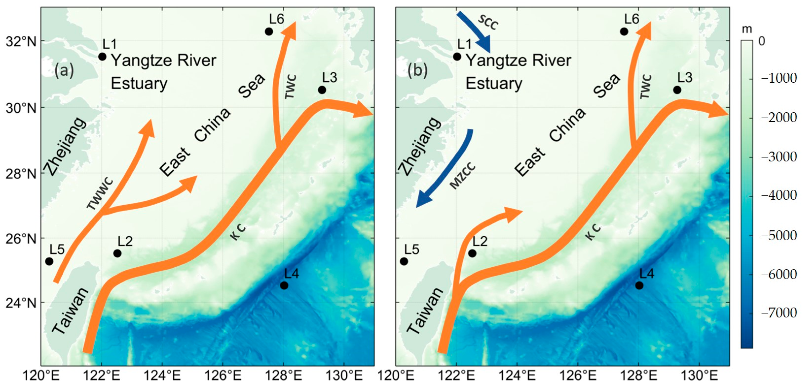
2. Data
3. Method
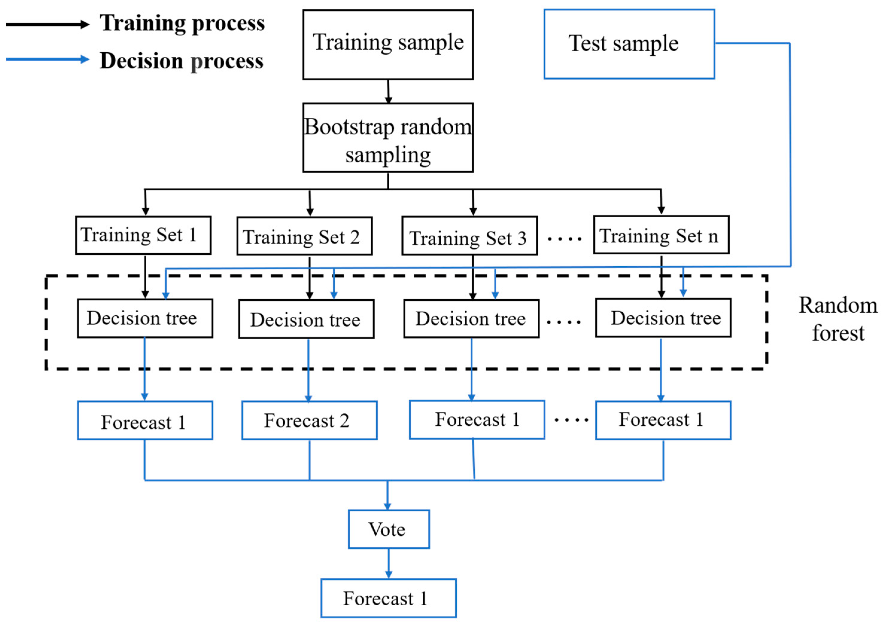
3.1. Random Forest
3.2. SA-ConvLSTM Model
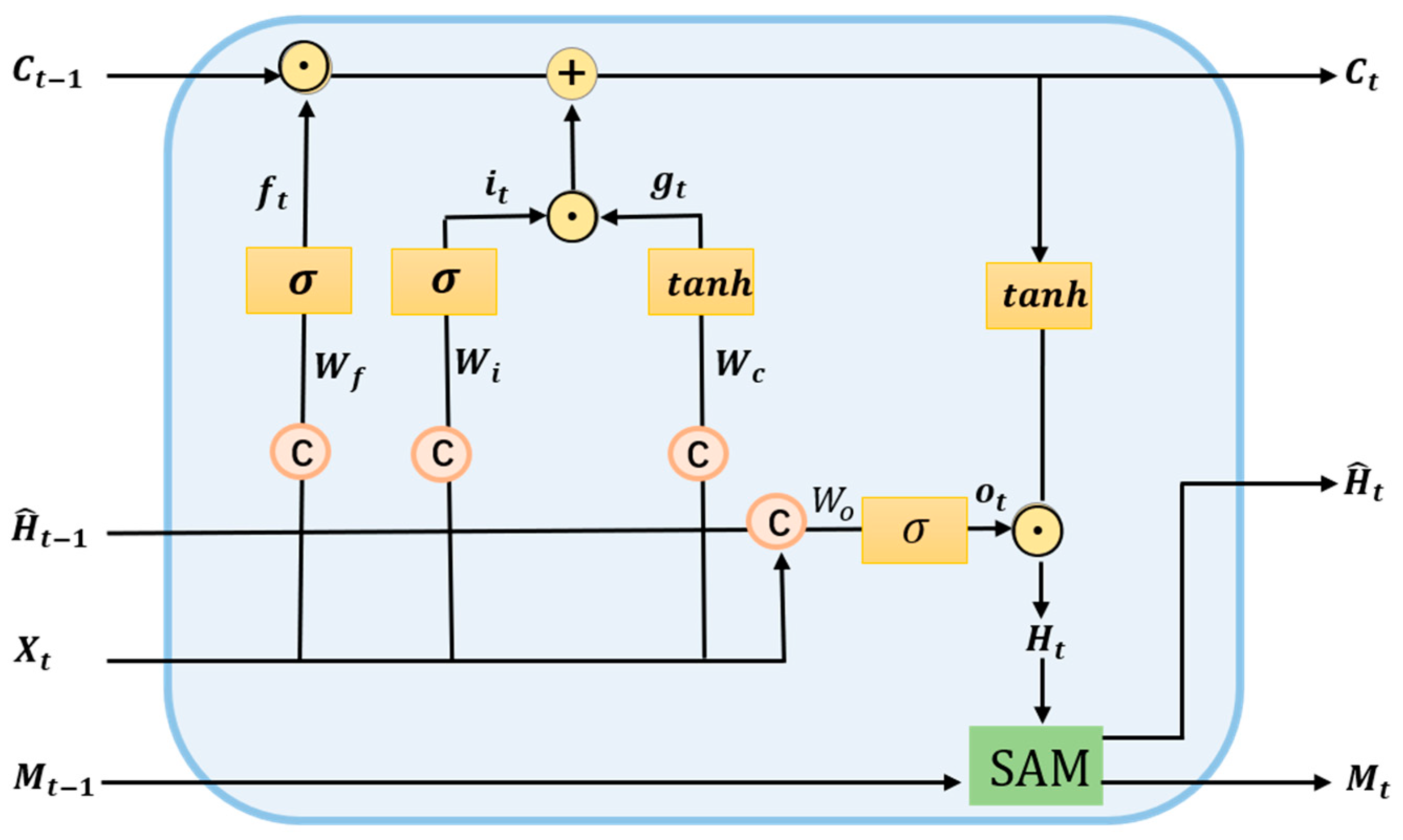
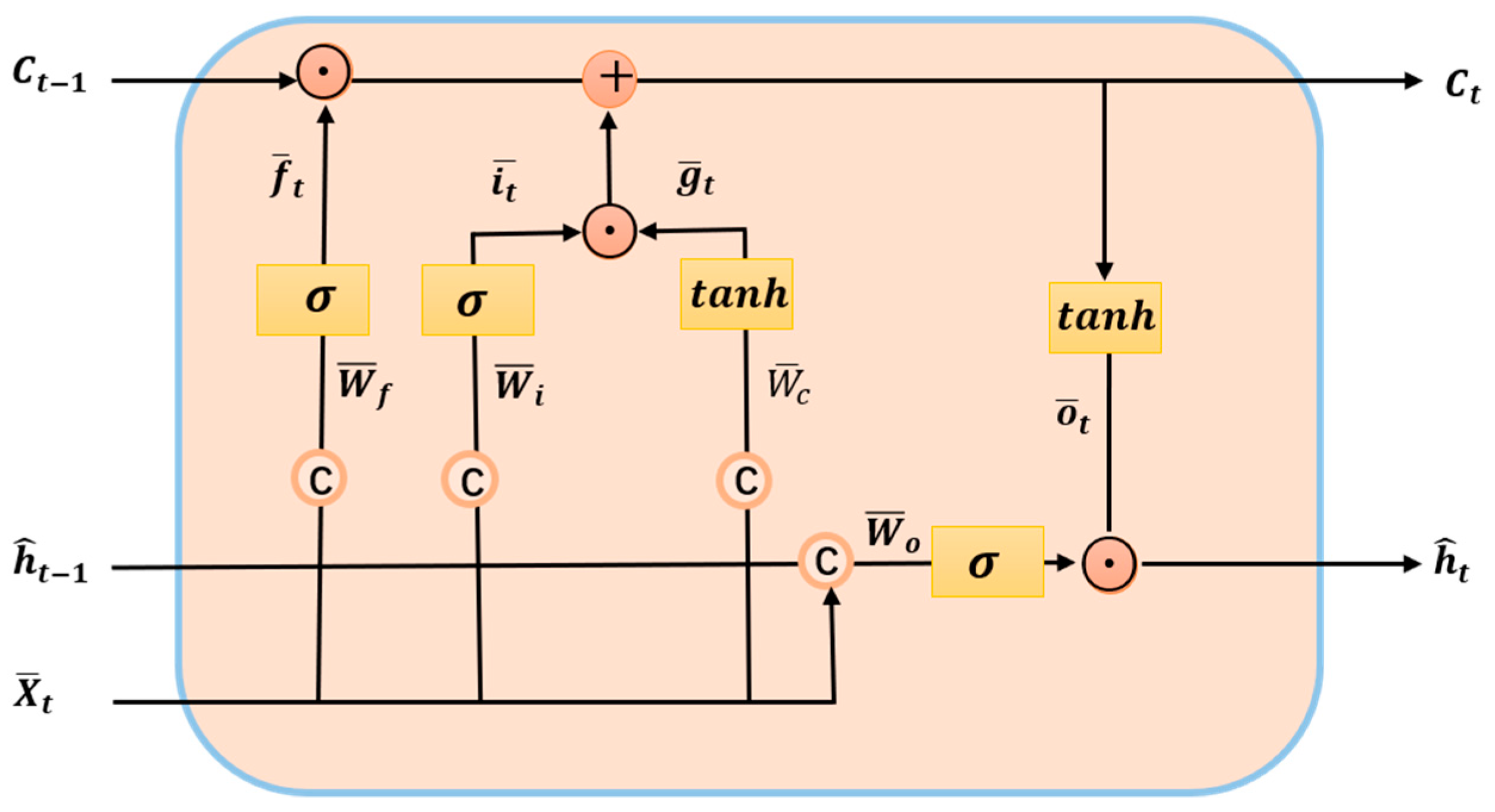
3.2.1. ConvLSTM Model
3.2.2. Self-Attention Memory Module
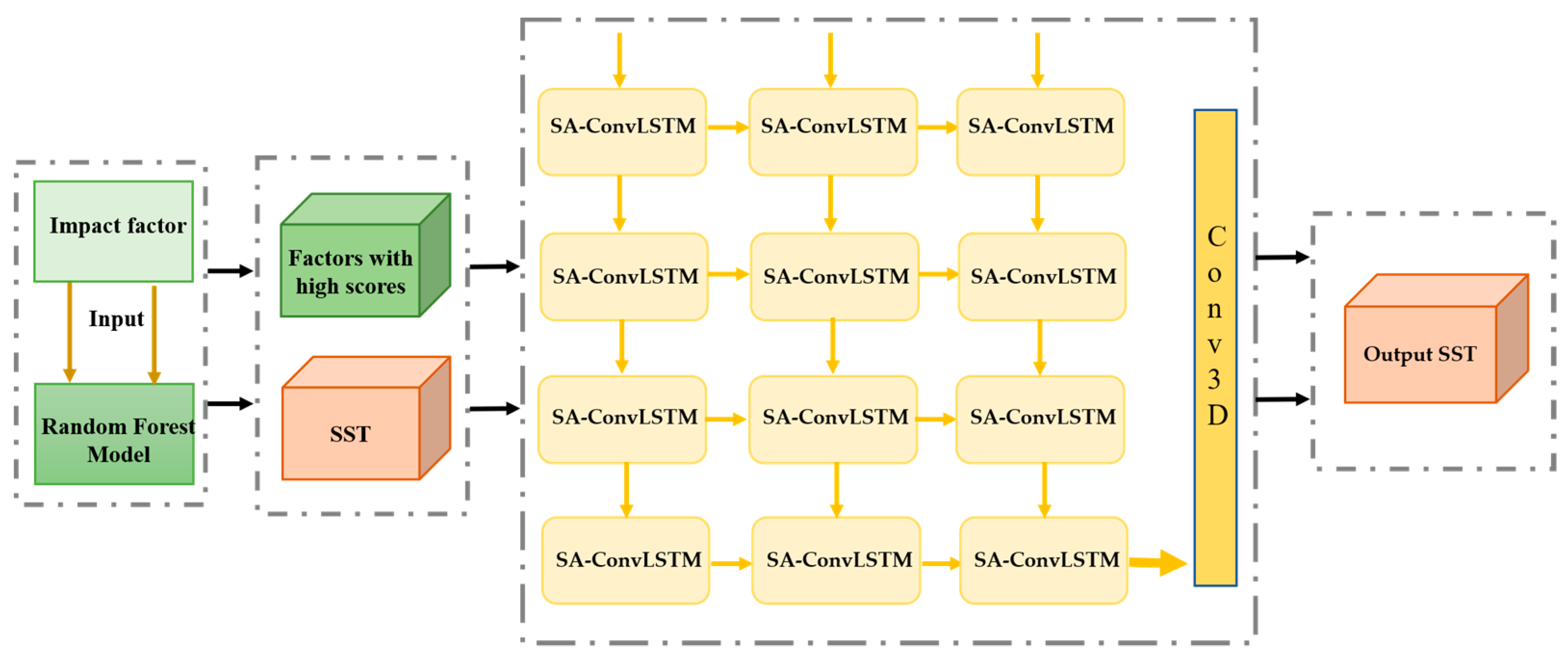
3.3. Model Construction
3.4. Evaluation Functions
4. Analysis of Results
4.1. Feature Importance Assessment for Random Forests
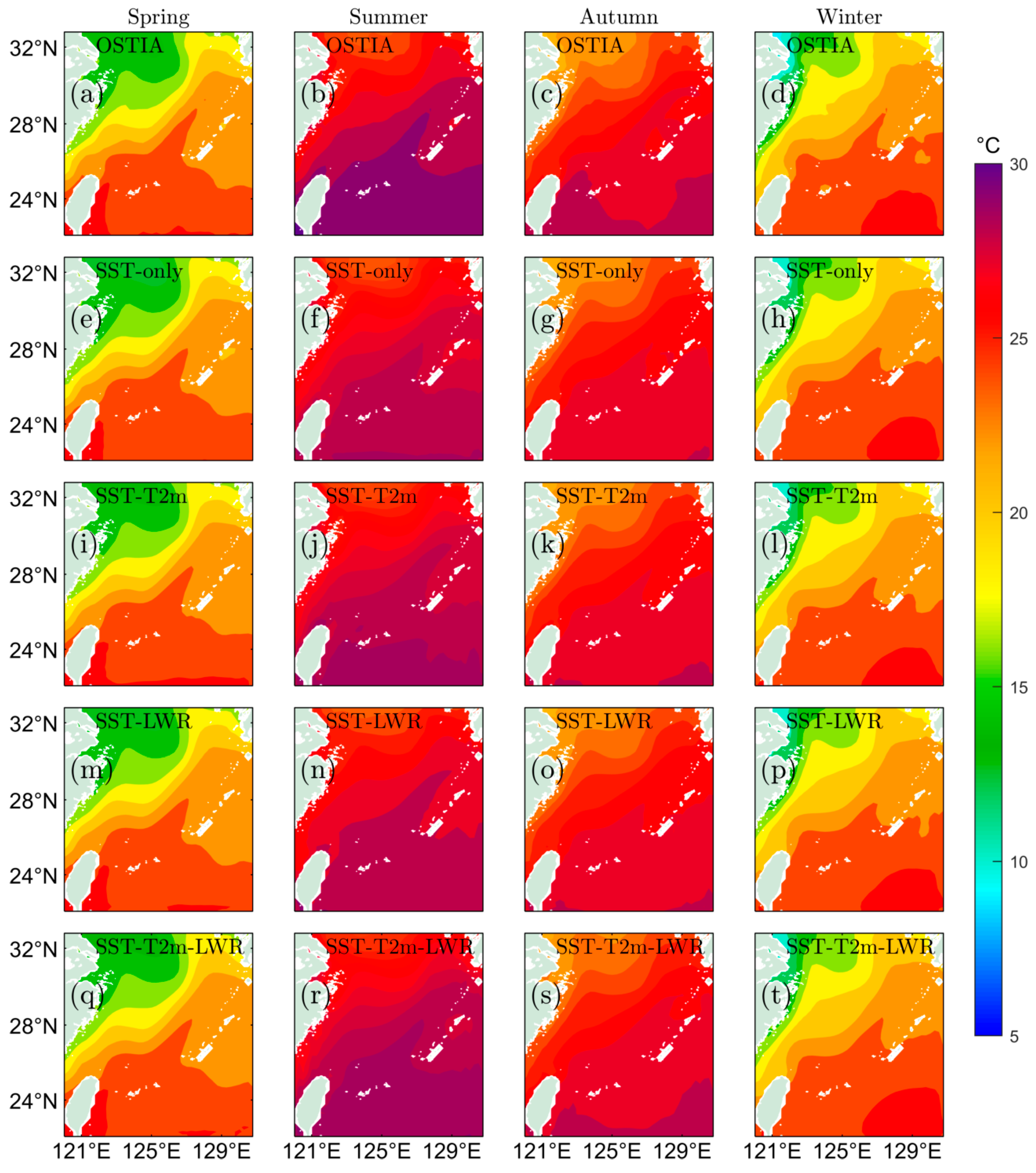
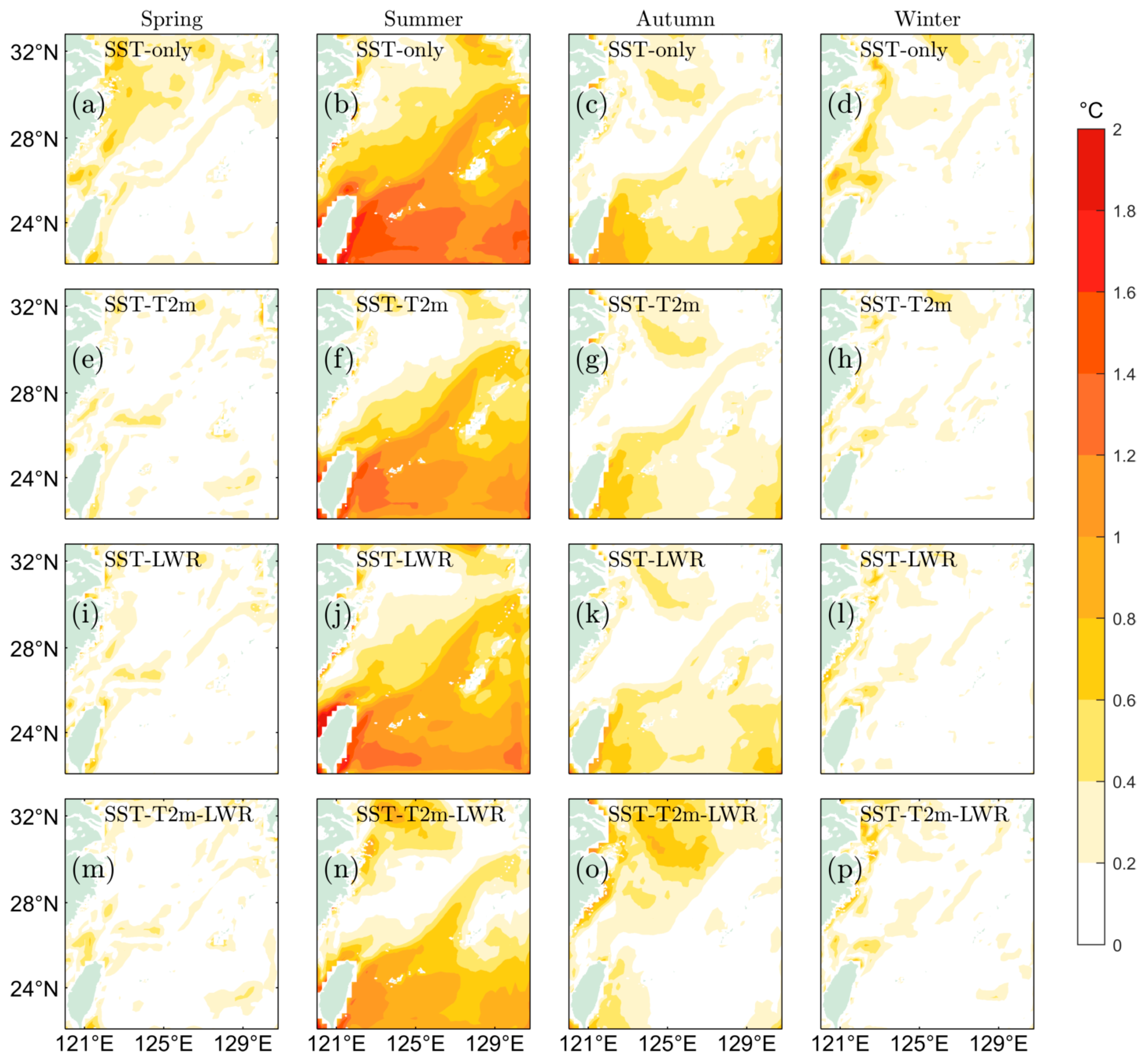
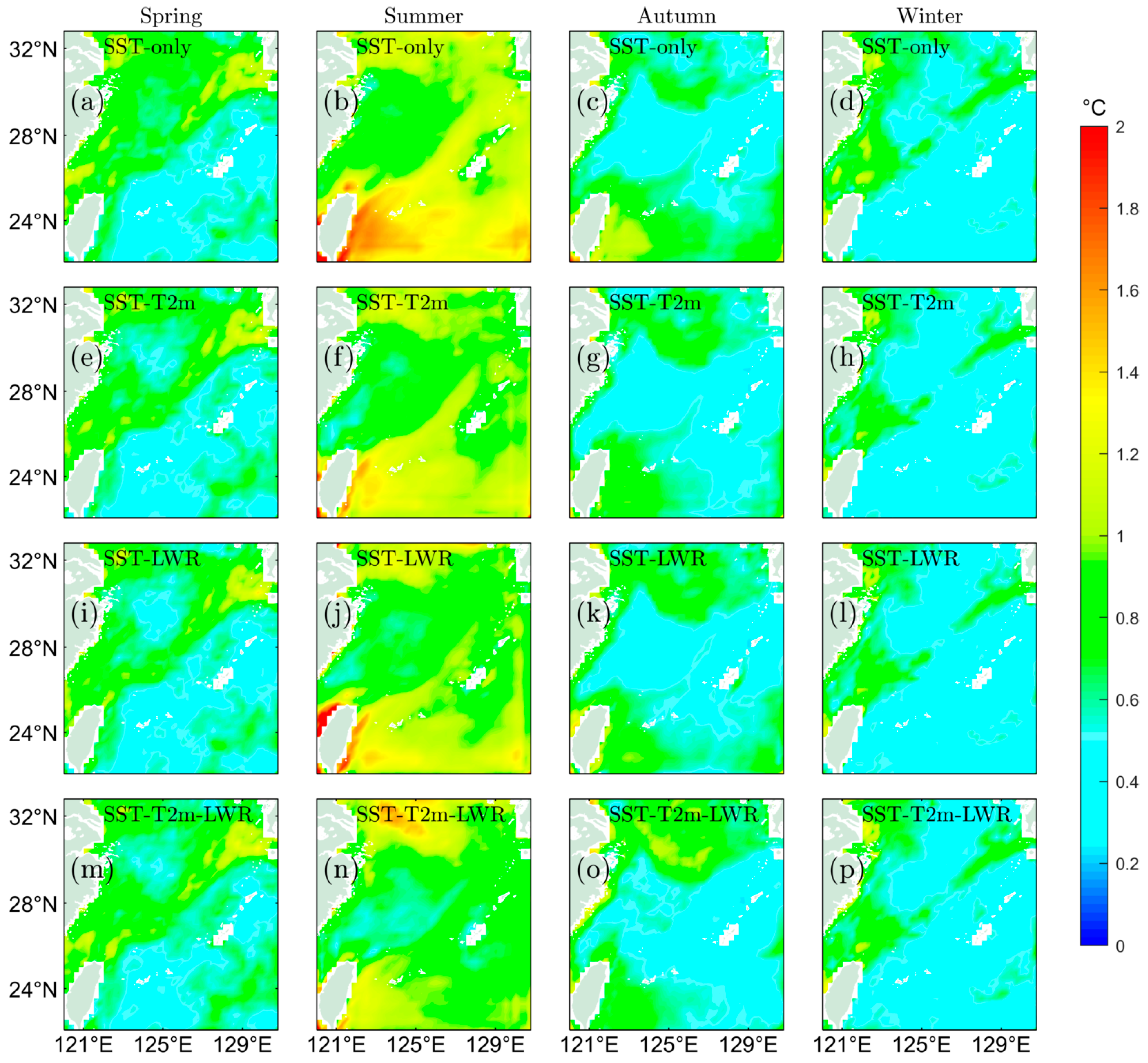
4.2. Spatial Variation Analysis of Prediction Results from SA-ConvLSTM Models
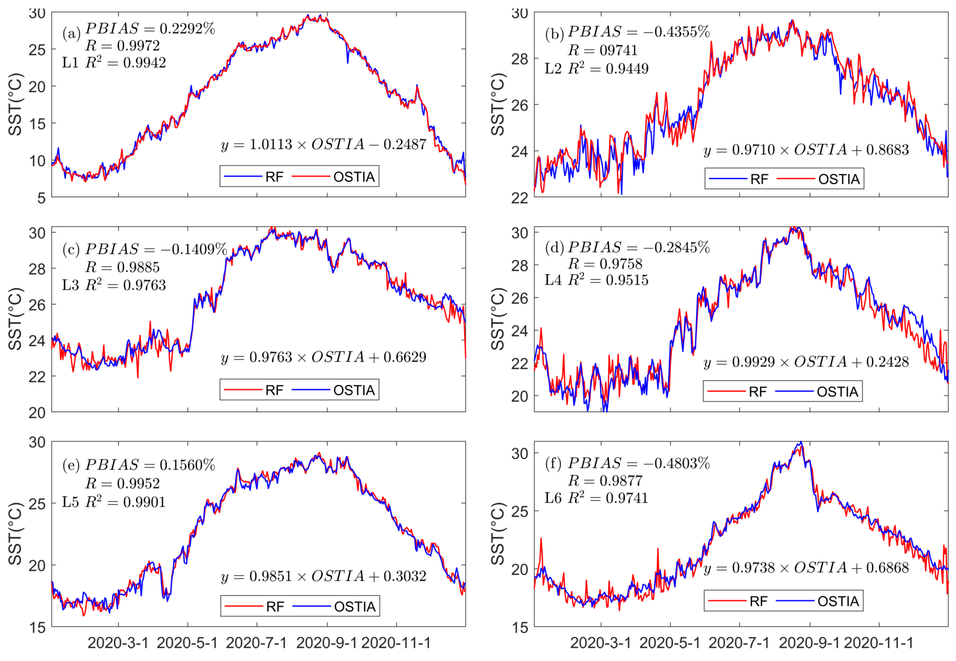
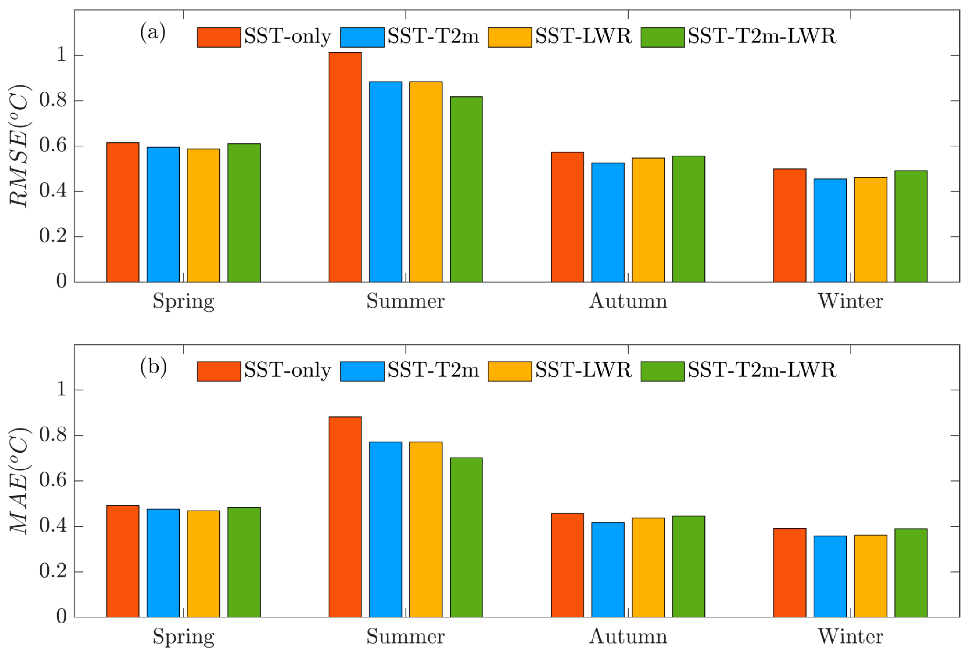
4.3. Temporal Variation Analysis of Prediction Results from SA-ConvLSTM Models
5. Discussion
6. Conclusions
Author Contributions
Funding
Institutional Review Board Statement
Informed Consent Statement
Data Availability Statement
Conflicts of Interest
References
- Herbert, T.D.; Peterson, L.C.; Lawrence, K.T.; Liu, Z. Tropical Ocean Temperatures over the Past 3.5 Million Years. Science 2010, 328, 1530–1534. [Google Scholar] [CrossRef] [PubMed]
- Bouali, M.; Sato, O.T.; Polito, P.S. Temporal trends in sea surface temperature gradients in the South Atlantic Ocean. Remote Sens. Environ. 2017, 194, 100–114. [Google Scholar] [CrossRef]
- Yao, S.-L.; Luo, J.-J.; Huang, G.; Wang, P. Distinct global warming rates tied to multiple ocean surface temperature changes. Nat. Clim. Chang. 2017, 7, 486–491. [Google Scholar] [CrossRef]
- Lin, X.; Shi, J.; Jiang, G.; Liu, Z. The influence of ocean waves on sea surface current field and sea surface temperature under the typhoon background. Mar. Sci. Bull. 2018, 37, 396–403. [Google Scholar] [CrossRef]
- Nagasoe, S.; Kim, D.-I.; Shimasaki, Y.; Oshima, Y.; Yamaguchi, M.; Honjo, T. Effects of temperature, salinity and irradiance on the growth of the red tide dinoflagellate Gyrodinium instriatum Freudenthal et Lee. Harmful Algae 2006, 5, 20–25. [Google Scholar] [CrossRef]
- Li, S.; Goddard, L.; DeWitt, D.G. Predictive Skill of AGCM Seasonal Climate Forecasts Subject to Different SST Prediction Methodologies. J. Clim. 2008, 21, 2169–2186. [Google Scholar] [CrossRef]
- Solanki, H.U.; Bhatpuria, D.; Chauhan, P. Signature analysis of satellite derived SSHa, SST and chlorophyll concentration and their linkage with marine fishery resources. J. Mar. Syst. 2015, 150, 12–21. [Google Scholar] [CrossRef]
- Jiao, N.; Zhang, Y.; Zeng, Y.; Gardner, W.D.; Mishonov, A.V.; Richardson, M.J.; Hong, N.; Pan, D.; Yan, X.-H.; Jo, Y.-H.; et al. Ecological anomalies in the East China Sea: Impacts of the Three Gorges Dam? Water Res. 2007, 41, 1287–1293. [Google Scholar] [CrossRef] [PubMed]
- Patil, K.; Deo, M.C. Prediction of daily sea surface temperature using efficient neural networks. Ocean Dyn. 2017, 67, 357–368. [Google Scholar] [CrossRef]
- Wei, X.; Xiang, Y.; Wu, H.; Zhou, S.; Sun, Y.; Ma, M.; Huang, X. AI-GOMS: Large AI-Driven Global Ocean Modeling System. arXiv 2023, arXiv:2308.03152. [Google Scholar] [CrossRef]
- Stockdale, T.N.; Balmaseda, M.A.; Vidard, A. Tropical Atlantic SST Prediction with Coupled Ocean–Atmosphere GCMs. J. Clim. 2006, 19, 6047–6061. [Google Scholar] [CrossRef]
- Krishnamurti, T.; Chakraborty, A.; Krishnamurti, R.; Dewar, W.; Clayson, C. Seasonal Prediction of Sea Surface Temperature Anomalies Using a Suite of 13 Coupled Atmosphere–Ocean Models. J. Clim. 2006, 19, 6069–6088. [Google Scholar] [CrossRef]
- Song, G.; Xianqing, L.; Wang, H. Sea Surface Temperature Simulation of Tropical and North Pacific Basins Using a Hybrid Coordinate Ocean Model (HYCOM). Mar. Sci. Bull. 2008, 10, 1–14. [Google Scholar]
- Zhang, X.; Zhang, W.; Li, Y. Characteristics of the sea temperature in the North Yellow Sea. Mar. Forecast. 2015, 32, 89–97. [Google Scholar]
- Qian, Z.; Tian, J.; Cao, C.; Wang, Q. The numerical simulation and the assimilation technique of the current and the temperature field in the Bohai Sea, the Huanghai Sea and the East China Sea. Haiyang Xuebao 2005, 27, 1–6. [Google Scholar]
- Xiao, C.; Chen, N.; Hu, C.; Wang, K.; Xu, Z.; Cai, Y.; Xu, L.; Chen, Z.; Gong, J. A spatiotemporal deep learning model for sea surface temperature field prediction using time-series satellite data. Environ. Model. Softw. 2019, 120, 104502. [Google Scholar] [CrossRef]
- Wie, L.; Guan, L.; Qu, L.; Li, L. Prediction of Sea Surface Temperature in the South China Sea by Artificial Neural Networks. In Proceedings of the IGARSS 2019—2019 IEEE International Geoscience and Remote Sensing Symposium, Yokohama, Japan, 28 July–2 August 2019; pp. 8158–8161. [Google Scholar] [CrossRef]
- Garcia-Gorriz, E.; Garcia-Sanchez, J. Prediction of sea surface temperatures in the western Mediterranean Sea by neural networks using satellite observations. Geophys. Res. Lett. 2007, 34, L11603. [Google Scholar] [CrossRef]
- Patil, K.; Deo, M.C. Basin-Scale Prediction of Sea Surface Temperature with Artificial Neural Networks. J. Atmos. Ocean. Technol. 2018, 35, 1441–1455. [Google Scholar] [CrossRef]
- Zheng, G.; Li, X.; Zhang, R.H.; Liu, B. Purely satellite data-driven deep learning forecast of complicated tropical instability waves. Sci. Adv. 2020, 6, eaba1482. [Google Scholar] [CrossRef]
- Xue, Y.; Leetmaa, A. Forecasts of tropical Pacific SST and sea level using a Markov model. Geophys. Res. Lett. 2000, 27, 2701–2704. [Google Scholar] [CrossRef]
- Laepple, T.; Jewson, S.; Meagher, J.; O’Shay, A.; Penzer, J. Five year prediction of Sea Surface Temperature in the Tropical Atlantic: A comparison of simple statistical methods. arXiv 2007, arXiv:physics/0701162. [Google Scholar] [CrossRef]
- Kug, J.-S.; Kang, I.-S.; Lee, J.-Y.; Jhun, J.-G. A statistical approach to Indian Ocean sea surface temperature prediction using a dynamical ENSO prediction. Geophys. Res. Lett. 2004, 31, L09212. [Google Scholar] [CrossRef]
- Peng, Y.; Wang, Q.; Yuan, C.; Lin, K. Review of Research on Data Mining in Application of Meteorological Forecasting. J. Arid Meteorol. 2015, 33, 19–27. Available online: http://www.ghqx.org.cn/EN/10.11755/j.issn.1006-7639(2015)-01-0019 (accessed on 13 October 2022).
- Chaudhari, S.; Balasubramanian, R.; Gangopadhyay, A. Upwelling Detection in AVHRR Sea Surface Temperature (SST) Images using Neural-Network Framework. In Proceedings of the IGARSS 2008—2008 IEEE International Geoscience and Remote Sensing Symposium, Boston, MA, USA, 7–11 July 2008; pp. IV-926–IV-929. [Google Scholar] [CrossRef]
- Wu, Z.; Jiang, C.; Conde, M.; Deng, B.; Chen, J. Hybrid improved empirical mode decomposition and BP neural network model for the prediction of sea surface temperature. Ocean Sci. 2019, 15, 349–360. [Google Scholar] [CrossRef]
- Tangang, F.T.; Hsieh, W.W.; Tang, B. Forecasting regional sea surface temperatures in the tropical Pacific by neural network models, with wind stress and sea level pressure as predictors. J. Geophys. Res. Oceans 1998, 103, 7511–7522. [Google Scholar] [CrossRef]
- Wu, A.; Hsieh, W.W.; Tang, B. Neural network forecasts of the tropical Pacific sea surface temperatures. Neural Netw. 2006, 19, 145–154. [Google Scholar] [CrossRef] [PubMed]
- Tripathi, K.C.; Das, M.L.; Sahai, A. Predictability of sea surface temperature anomalies in the Indian Ocean using artificial neural networks. Indian J. Mar. Sci. 2006, 35, 210–220. [Google Scholar]
- Aparna, S.G.; D’Souza, S.; Arjun, N.B. Prediction of daily sea surface temperature using artificial neural networks. Int. J. Remote Sens. 2018, 39, 4214–4231. [Google Scholar] [CrossRef]
- Gupta, S.M.; Malmgren, B. Comparison of the accuracy of SST estimates by artificial neural networks (ANN) and other quantitative methods using radiolarian data from the Antarctic and Pacific Oceans. Earth Sci. India 2009, 2, 52–75. [Google Scholar]
- Hou, S.; Li, W.; Liu, T.; Zhou, S.; Guan, J.; Qin, R.; Wang, Z. MIMO: A Unified Spatio-Temporal Model for Multi-Scale Sea Surface Temperature Prediction. Remote Sens. 2022, 14, 2371. [Google Scholar] [CrossRef]
- Zhang, Q.; Wang, H.; Dong, J.; Zhong, G.; Sun, X. Prediction of Sea Surface Temperature Using Long Short-Term Memory. IEEE Geosci. Remote Sens. Lett. 2017, 14, 1745–1749. [Google Scholar] [CrossRef]
- Xiao, C.; Chen, N.; Hu, C.; Wang, K.; Gong, J.; Chen, Z. Short and mid-term sea surface temperature prediction using time-series satellite data and LSTM-AdaBoost combination approach. Remote Sens. Environ. 2019, 233, 111358. [Google Scholar] [CrossRef]
- He, Q.; Hu, Z.; Xu, H.; Song, W.; Du, Y. Sea Surface Temperature Prediction Method Based on Empirical Mode Decomposition-Gated Recurrent Unit Model. Laser Optoelectron. Prog. 2021, 58, 9. [Google Scholar] [CrossRef]
- Ham, Y.-G.; Kim, J.-H.; Luo, J.-J. Deep learning for multi-year ENSO forecasts. Nature 2019, 573, 568–572. [Google Scholar] [CrossRef] [PubMed]
- Shi, X.; Chen, Z.; Wang, H.; Yeung, D.-Y.; Wong, W.-K.; Woo, W.-C. Convolutional LSTM Network: A machine learning approach for precipitation nowcasting. In Proceedings of the 28th International Conference on Neural Information Processing Systems, Montreal, QC, Canada, 7–12 December 2015; Volume 1, pp. 802–810. [Google Scholar] [CrossRef]
- Zhang, K.; Geng, X.; Yan, X.H. Prediction of 3-D Ocean Temperature by Multilayer Convolutional LSTM. IEEE Geosci. Remote Sens. Lett. 2020, 17, 1303–1307. [Google Scholar] [CrossRef]
- Luo, W.; Li, Y.; Urtasun, R.; Zemel, R. Understanding the effective receptive field in deep convolutional neural networks. In Proceedings of the 30th International Conference on Neural Information Processing Systems, Barcelona, Spain, 5–10 December 2016; pp. 4905–4913. [Google Scholar] [CrossRef]
- Lin, Z.; Li, M.; Zheng, Z.; Cheng, Y.; Yuan, C. Self-Attention ConvLSTM for Spatiotemporal Prediction. Proc. AAAI Conf. Artif. Intell. 2020, 34, 11531–11538. [Google Scholar] [CrossRef]
- Donlon, C.J.; Martin, M.; Stark, J.; Roberts-Jones, J.; Fiedler, E.; Wimmer, W. The Operational Sea Surface Temperature and Sea Ice Analysis (OSTIA) system. Remote Sens. Environ. 2012, 116, 140–158. [Google Scholar] [CrossRef]
- Stewart, R.H. Introduction to Physical Oceanography; Prentice Hall: Upper Saddle River, NJ, USA, 2008; pp. 51–52. [Google Scholar] [CrossRef]
- Breiman, L. Bagging Predictors. Mach. Learn. 1996, 24, 123–140. [Google Scholar] [CrossRef]
- Breiman, L. Random Forests. Mach. Learn. 2001, 45, 5–32. [Google Scholar] [CrossRef]
- Belgiu, M.; Drăguţ, L.D. Random forest in remote sensing: A review of applications and future directions. ISPRS J. Photogramm. Remote Sens. 2016, 114, 24–31. [Google Scholar] [CrossRef]
- Chen, S.; Yu, L.; Zhang, C.; Wu, Y.; Li, T. Environmental impact assessment of multi-source solid waste based on a life cycle assessment, principal component analysis, and random forest algorithm. J. Environ. Manag. 2023, 339, 117942. [Google Scholar] [CrossRef] [PubMed]
- Morse-McNabb, E.M.; Hasan, M.F.; Karunaratne, S. A Multi-Variable Sentinel-2 Random Forest Machine Learning Model Approach to Predicting Perennial Ryegrass Biomass in Commercial Dairy Farms in Southeast Australia. Remote Sens. 2023, 15, 2915. [Google Scholar] [CrossRef]
- Wang, Y.; Chen, X.; Wang, Z.; Gao, M.; Wang, L. Integrating SBAS-InSAR and Random Forest for Identifying and Controlling Land Subsidence and Uplift in a Multi-Layered Porous System of North China Plain. Remote Sens. 2024, 16, 830. [Google Scholar] [CrossRef]
- Su, H.; Li, W.; Yan, X.-H. Retrieving temperature anomaly in the global subsurface and deeper ocean from satellite observations. J. Geophys. Res. Oceans 2018, 123, 399–410. [Google Scholar] [CrossRef]
- Cui, H.; Tang, D.; Mei, W.; Liu, H.; Sui, Y.; Gu, X. Predicting tropical cyclone-induced sea surface temperature responses using machine learning. Geophys. Res. Lett. 2023, 50, e2023GL104171. [Google Scholar] [CrossRef]
- Chen, C.-T.A.; Sheu, D.D. Does the Taiwan Warm Current originate in the Taiwan Strait in wintertime? J. Geophys. Res. Oceans 2006, 111, C04005. [Google Scholar] [CrossRef]
- Chen, C.-T.A. Rare northward flow in the Taiwan Strait in winter: A note. Cont. Shelf Res. 2003, 23, 387–391. [Google Scholar] [CrossRef]
- Sonnewald, M.; Lguensat, R.; Jones, D.C.; Dueben, P.D.; Brajard, J.; Balaji, V. Bridging observations, theory and numerical simulation of the ocean using machine learning. Environ. Res. Lett. 2021, 16, 073008. [Google Scholar] [CrossRef]
- Qiao, F.; Yuan, Y.; Yang, Y.; Zheng, Q.; Xia, C.; Ma, J. Wave-induced mixing in the upper ocean: Distribution and application to a global ocean circulation model. Geophys. Res. Lett. 2004, 31, L11303. [Google Scholar] [CrossRef]
- Huang, C.J.; Qiao, F.; Chen, S.; Xue, Y.; Guo, J. Observation and Parameterization of Broadband Sea Surface Albedo. J. Geophys. Res. Oceans 2019, 124, 4480–4491. [Google Scholar] [CrossRef]
- Lin, J. Numerical Simulation of Three-Dimensional Current Field and Temperature Field of the Bohai Sea, Yellow Sea and the East China Sea. Master’s Thesis, Ocean University of China, Qingdao, China, 2004. Available online: https://www.dissertationtopic.net/doc/1278630 (accessed on 18 January 2024).
- Jia, X.; Ji, Q.; Han, L.; Liu, Y.; Han, G.; Lin, X. Prediction of Sea Surface Temperature in the East China Sea Based on LSTM Neural Network. Remote Sens. 2022, 14, 3300. [Google Scholar] [CrossRef]
- Xu, S.; Dai, D.; Cui, X.; Yin, X.; Jiang, S.; Pan, H.; Wang, G. A deep leaning approach to predict sea surface temperature based on multiple modes. Ocean Modell. 2023, 181, 102158. [Google Scholar] [CrossRef]
- Yu, X.; Shi, S.; Xu, L.; Liu, Y.; Miao, Q.; Sun, M. A Novel Method for Sea Surface Temperature Prediction Based on Deep Learning. Math. Probl. Eng. 2020, 2020, 6387173. [Google Scholar] [CrossRef]


| SST-Only | SST-T2m | SST-LWR | SST-T2m-LWR | |
|---|---|---|---|---|
| MAE | 0.5563 | 0.5064 | 0.5106 | 0.5059 |
| RMSE | 0.7221 | 0.6506 | 0.6540 | 0.6445 |
| 0% | 9.9% | 9.43% | 10.75% | |
| 0% | 8.97% | 8.21% | 9.06% |
Disclaimer/Publisher’s Note: The statements, opinions and data contained in all publications are solely those of the individual author(s) and contributor(s) and not of MDPI and/or the editor(s). MDPI and/or the editor(s) disclaim responsibility for any injury to people or property resulting from any ideas, methods, instructions or products referred to in the content. |
© 2024 by the authors. Licensee MDPI, Basel, Switzerland. This article is an open access article distributed under the terms and conditions of the Creative Commons Attribution (CC BY) license (https://creativecommons.org/licenses/by/4.0/).
Share and Cite
Ji, Q.; Jia, X.; Jiang, L.; Xie, M.; Meng, Z.; Wang, Y.; Lin, X. Contribution of Atmospheric Factors in Predicting Sea Surface Temperature in the East China Sea Using the Random Forest and SA-ConvLSTM Model. Atmosphere 2024, 15, 670. https://doi.org/10.3390/atmos15060670
Ji Q, Jia X, Jiang L, Xie M, Meng Z, Wang Y, Lin X. Contribution of Atmospheric Factors in Predicting Sea Surface Temperature in the East China Sea Using the Random Forest and SA-ConvLSTM Model. Atmosphere. 2024; 15(6):670. https://doi.org/10.3390/atmos15060670
Chicago/Turabian StyleJi, Qiyan, Xiaoyan Jia, Lifang Jiang, Minghong Xie, Ziyin Meng, Yuting Wang, and Xiayan Lin. 2024. "Contribution of Atmospheric Factors in Predicting Sea Surface Temperature in the East China Sea Using the Random Forest and SA-ConvLSTM Model" Atmosphere 15, no. 6: 670. https://doi.org/10.3390/atmos15060670
APA StyleJi, Q., Jia, X., Jiang, L., Xie, M., Meng, Z., Wang, Y., & Lin, X. (2024). Contribution of Atmospheric Factors in Predicting Sea Surface Temperature in the East China Sea Using the Random Forest and SA-ConvLSTM Model. Atmosphere, 15(6), 670. https://doi.org/10.3390/atmos15060670