
Frequency of Italian Record-Breaking Floods over the Last Century (1911–2020)

 , , , ,
Abstract
:1. Introduction
2. Data and Methods
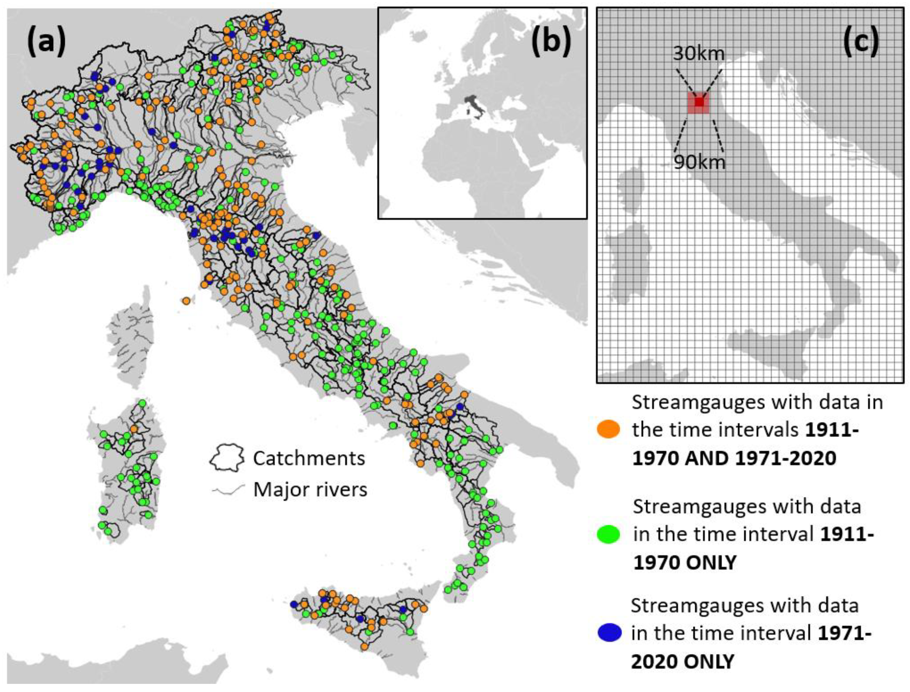
2.1. Study Area
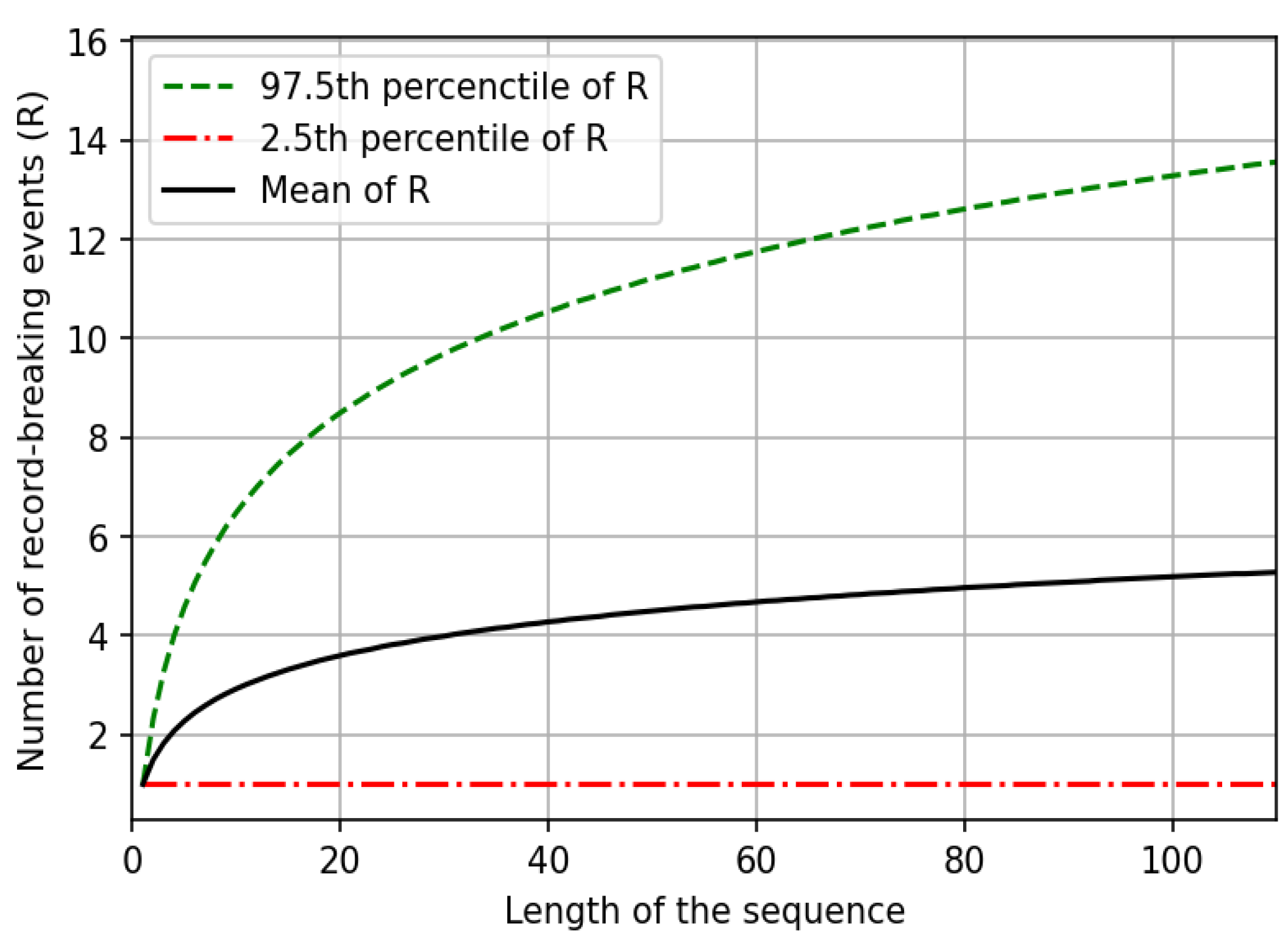
2.2. Number of Record-Breaking Events in Independent and Identically Distributed (iid) Series
2.3. Testing the Statistical Significance of the Deviation in the Average Number of Records in Pooling-Groups of AMS of Flood Flows Relative to What Is Expected under the iid Hypothesis
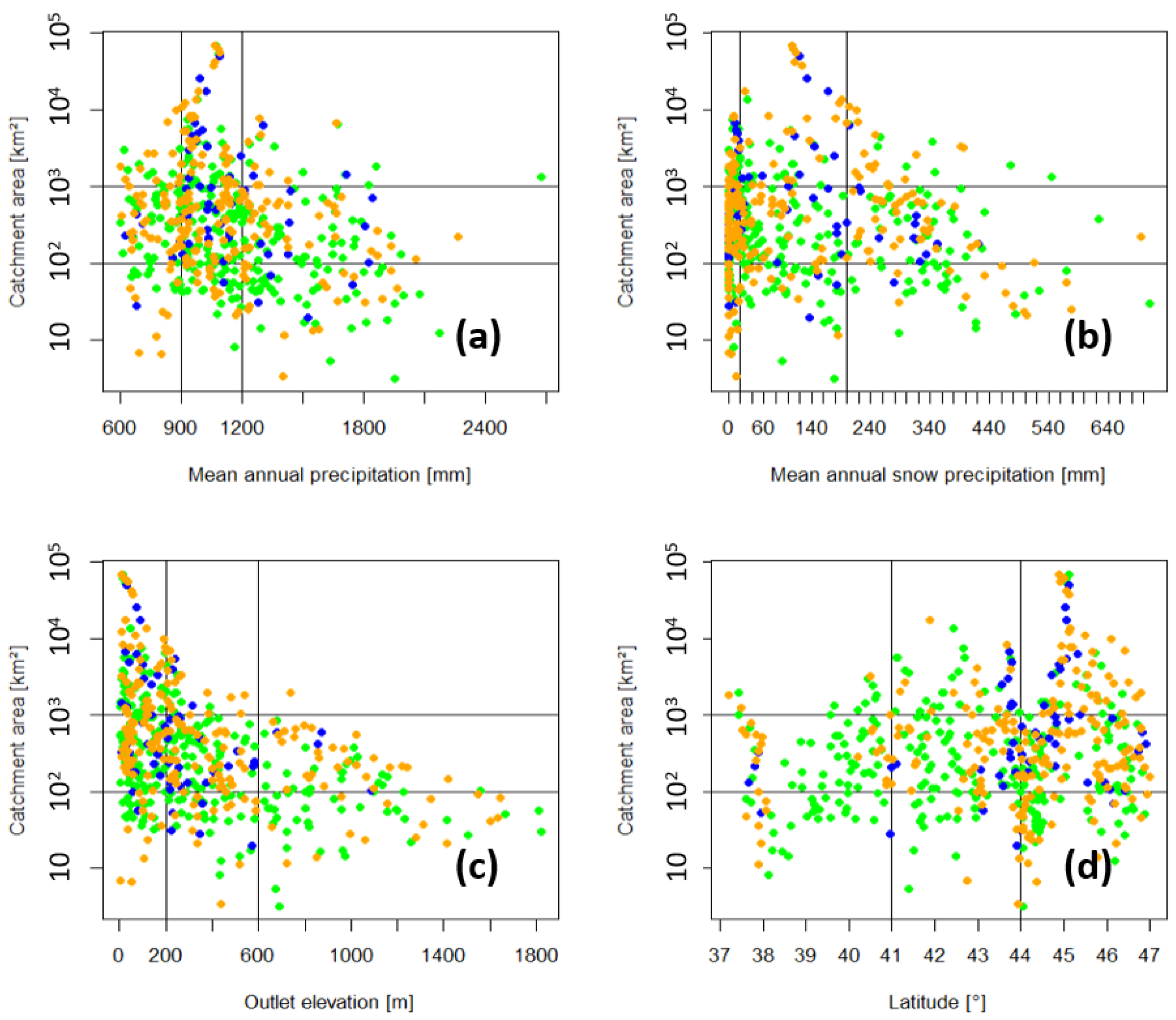
2.4. Criteria for Pooling-Groups Definition
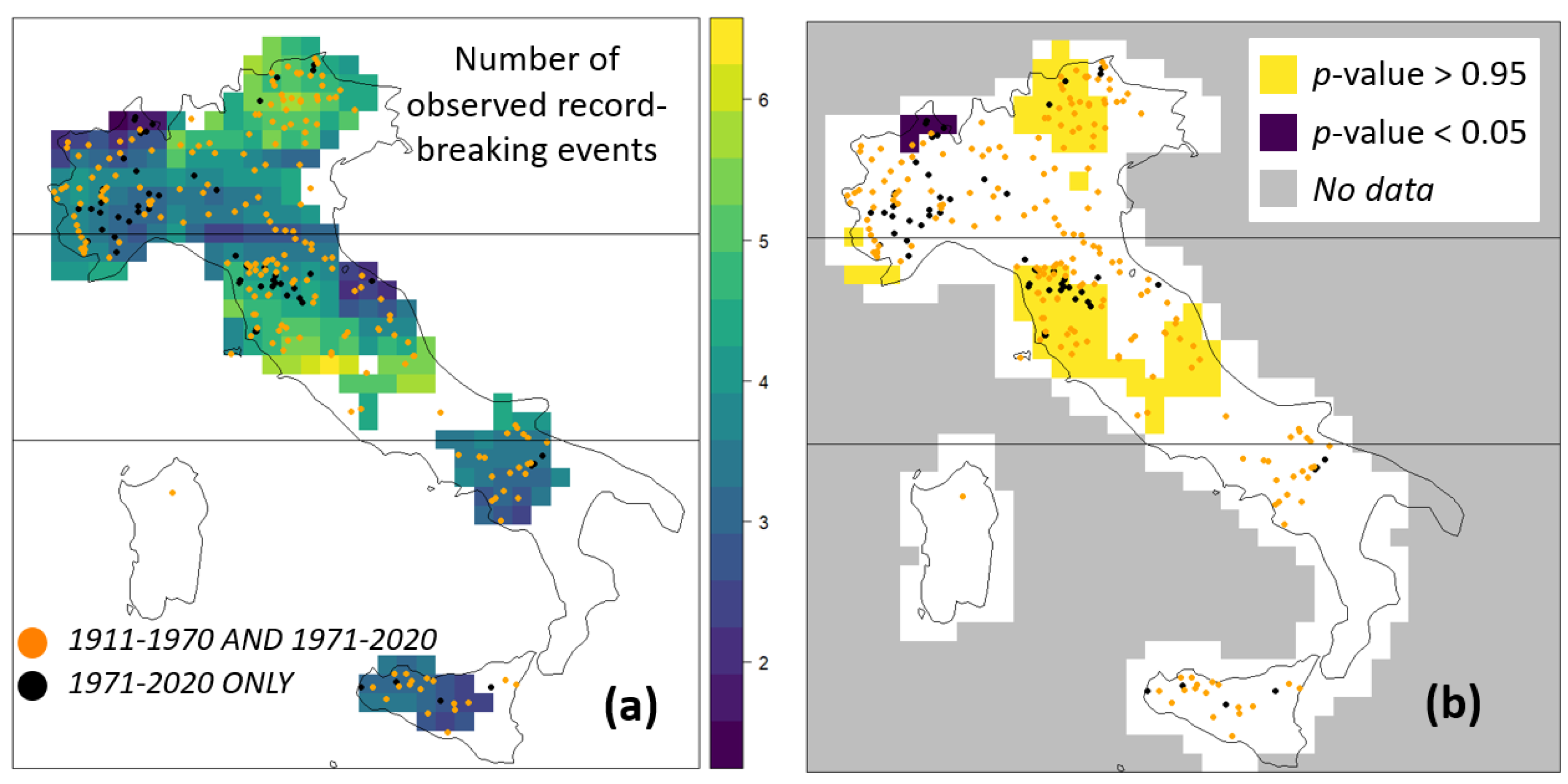
3. Results
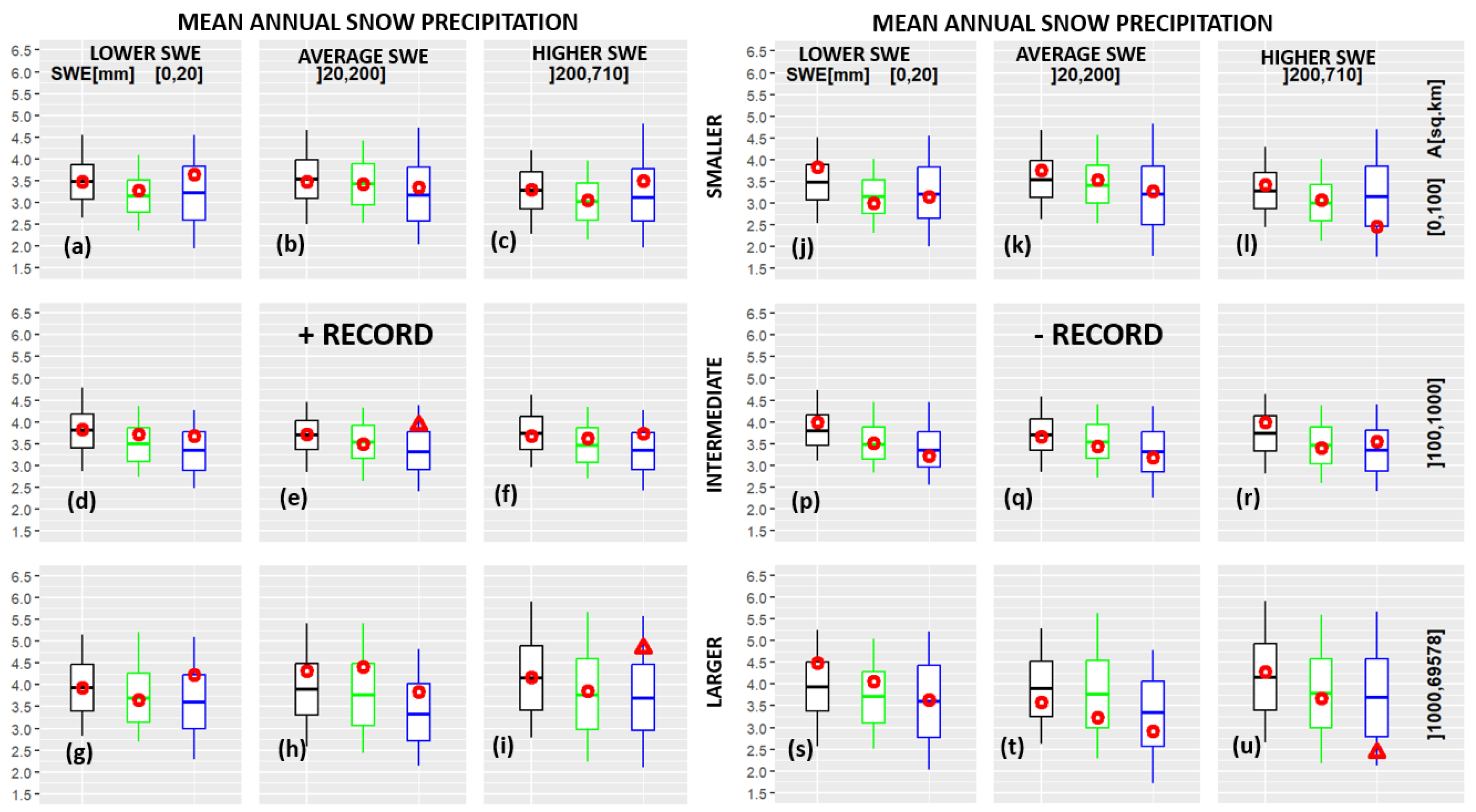
3.1. Pooling-Groups of Hydrologically Similar Catchments
3.2. Pooling-Groups of Spatially Close Catchments
4. Discussion
5. Conclusions
Author Contributions
Funding
Institutional Review Board Statement
Informed Consent Statement
Data Availability Statement
Acknowledgments
Conflicts of Interest
References
- Jongman, B.; Koks, E.E.; Husby, T.G.; Ward, P.J. Increasing Flood Exposure in the Netherlands: Implications for Risk Financing. Nat. Hazards Earth Syst. Sci. 2014, 14, 1245–1255. [Google Scholar] [CrossRef]
- Guha-Sapir, D.; Hoyois, P.; Wallemacq, P.; Below, R. Annual Disaster Statistical Review 2016: The Numbers and Trends; Centre for Research on the Epidemiology of Disasters: Brussels, Belgium, 2016. [Google Scholar]
- Hirabayashi, Y.; Mahendran, R.; Koirala, S.; Konoshima, L.; Yamazaki, D.; Watanabe, S.; Kim, H.; Kanae, S. Global Flood Risk under Climate Change. Nat. Clim. Chang. 2013, 3, 816–821. [Google Scholar] [CrossRef]
- Do, H.X.; Westra, S.; Leonard, M. A Global-Scale Investigation of Trends in Annual Maximum Streamflow. J. Hydrol. 2017, 552, 28–43. [Google Scholar] [CrossRef]
- Alfieri, L.; Burek, P.; Feyen, L.; Forzieri, G. Global Warming Increases the Frequency of River Floods in Europe. Hydrol. Earth Syst. Sci. 2015, 19, 2247–2260. [Google Scholar] [CrossRef]
- Mediero, L.; Kjeldsen, T.R.; Macdonald, N.; Kohnova, S.; Merz, B.; Vorogushyn, S.; Wilson, D.; Alburquerque, T.; Blöschl, G.; Bogdanowicz, E.; et al. Identification of Coherent Flood Regions across Europe by Using the Longest Streamflow Records. J. Hydrol. 2015, 528, 341–360. [Google Scholar] [CrossRef]
- Berghuijs, W.R.; Aalbers, E.E.; Larsen, J.R.; Trancoso, R.; Woods, R.A. Recent Changes in Extreme Floods across Multiple Continents. Environ. Res. Lett. 2017, 12, 114035. [Google Scholar] [CrossRef]
- Bertola, M.; Viglione, A.; Vorogushyn, S.; Lun, D.; Merz, B.; Blöschl, G. Do Small and Large Floods Have the Same Drivers of Change? A Regional Attribution Analysis in Europe. Hydrol. Earth Syst. Sci. 2021, 25, 1347–1364. [Google Scholar] [CrossRef]
- Blöschl, G.; Kiss, A.; Viglione, A.; Barriendos, M.; Böhm, O.; Brázdil, R.; Coeur, D.; Demarée, G.; Llasat, M.C.; Macdonald, N.; et al. Current European Flood-Rich Period Exceptional Compared with Past 500 Years. Nature 2020, 583, 560–566. [Google Scholar] [CrossRef] [PubMed]
- Blöschl, G.; Hall, J.; Parajka, J.; Perdigão, R.A.P.; Merz, B.; Arheimer, B.; Aronica, G.T.; Bilibashi, A.; Bonacci, O.; Borga, M.; et al. Changing Climate Shifts Timing of European Floods. Science 2017, 357, 588–590. [Google Scholar] [CrossRef]
- Blöschl, G.; Hall, J.; Viglione, A.; Perdigão, R.A.P.; Parajka, J.; Merz, B.; Lun, D.; Arheimer, B.; Aronica, G.T.; Bilibashi, A.; et al. Changing Climate Both Increases and Decreases European River Floods. Nature 2019, 573, 108–111. [Google Scholar] [CrossRef]
- Venegas-Cordero, N.; Kundzewicz, Z.W.; Jamro, S.; Piniewski, M. Detection of Trends in Observed River Floods in Poland. J. Hydrol. Reg. Stud. 2022, 41, 101098. [Google Scholar] [CrossRef]
- Lintunen, K.; Kasvi, E.; Uvo, C.B.; Alho, P. Changes in the Discharge Regime of Finnish Rivers. J. Hydrol. Reg. Stud. 2024, 53, 101749. [Google Scholar] [CrossRef]
- Slater, L.J.; Villarini, G. Recent Trends in U.S. Flood Risk. Geophys. Res. Lett. 2016, 43, 12428–12436. [Google Scholar] [CrossRef]
- Tramblay, Y.; Mimeau, L.; Neppel, L.; Vinet, F.; Sauquet, E. Detection and Attribution of Flood Trends in Mediterranean Basins. Hydrol. Earth Syst. Sci. 2019, 23, 4419–4431. [Google Scholar] [CrossRef]
- Kay, A.L.; Crooks, S.M.; Davies, H.N.; Prudhomme, C.; Reynard, N.S. Probabilistic Impacts of Climate Change on Flood Frequency Using Response Surfaces I: England and Wales. Reg. Environ. Chang. 2014, 14, 1215–1227. [Google Scholar] [CrossRef]
- Prosdocimi, I.; Dupont, E.; Augustin, N.H.; Kjeldsen, T.R.; Simpson, D.P.; Smith, T.R. Areal Models for Spatially Coherent Trend Detection: The Case of British Peak River Flows. Geophys. Res. Lett. 2019, 46, 13054–13061. [Google Scholar] [CrossRef]
- Renard, B.; Lang, M.; Bois, P.; Dupeyrat, A.; Mestre, O.; Niel, H.; Sauquet, E.; Prudhomme, C.; Parey, S.; Paquet, E.; et al. Regional Methods for Trend Detection: Assessing Field Significance and Regional Consistency. Water Resour. Res. 2008, 44, 2007WR006268. [Google Scholar] [CrossRef]
- Nerantzaki, S.D.; Papalexiou, S.M. Assessing Extremes in Hydroclimatology: A Review on Probabilistic Methods. J. Hydrol. 2022, 605, 127302. [Google Scholar] [CrossRef]
- Ouarda, T.B.M.J.; Charron, C. Changes in the Distribution of Hydro-Climatic Extremes in a Non-Stationary Framework. Sci. Rep. 2019, 9, 8104. [Google Scholar] [CrossRef]
- Fischer, S.; Schumann, A.; Bühler, P. Timescale-Based Flood Typing to Estimate Temporal Changes in Flood Frequencies. Hydrol. Sci. J. 2019, 64, 1867–1892. [Google Scholar] [CrossRef]
- Hesarkazzazi, S.; Arabzadeh, R.; Hajibabaei, M.; Rauch, W.; Kjeldsen, T.R.; Prosdocimi, I.; Castellarin, A.; Sitzenfrei, R. Stationary vs. Non-Stationary Modelling of Flood Frequency Distribution across Northwest England. Hydrol. Sci. J. 2021, 66, 729–744. [Google Scholar] [CrossRef]
- Coles, S. An Introduction to Statistical Modeling of Extreme Values; Springer series in statistics; Springer: London, UK; New York, NY, USA, 2001; ISBN 978-1-85233-459-8. [Google Scholar]
- Wei, W.W.S. Time Series Analysis: Univariate and Multivariate Methods, 2nd ed.; Pearson Addison Wesley: Boston, MA, USA, 2006; ISBN 978-0-321-32216-6. [Google Scholar]
- Dalrymple, T. Flood-Frequency Analyses, Manual of Hydrology: Part 3; U.S. Geological Survey Water Supply Paper; United States Government Printing Office: Washington, DC, USA, 1960. [Google Scholar]
- Kendall, M.; Gibbons, J.D. Rank Correlation Methods: A Charles Griffin Title, 5th ed.; E. Arnold: London, UK; Melbourne, Australia; Auckland, New Zealand, 1990; ISBN 978-0-85264-305-1. [Google Scholar]
- Koutsoyiannis, D. Statistics of Extremes and Estimation of Extreme Rainfall: II. Empirical Investigation of Long Rainfall Records/Statistiques de Valeurs Extrêmes et Estimation de Précipitations Extrêmes: II. Recherche Empirique Sur de Longues Séries de Précipitations. Hydrol. Sci. J. 2004, 49, 4. [Google Scholar] [CrossRef]
- Papalexiou, S.M.; Koutsoyiannis, D. Battle of Extreme Value Distributions: A Global Survey on Extreme Daily Rainfall. Water Resour. Res. 2013, 49, 187–201. [Google Scholar] [CrossRef]
- Arnold, B.C.; Balakrishnan, N.; Nagaraja, H.N. Records, 1st ed.; Wiley Series in Probability and Statistics; Wiley: Hoboken, NJ, USA, 1998; ISBN 978-0-471-08108-1. [Google Scholar]
- Vogel, R.M.; Zafirakou-Koulouris, A.; Matalas, N.C. Frequency of Record-breaking Floods in the United States. Water Resour. Res. 2001, 37, 1723–1731. [Google Scholar] [CrossRef]
- Vogel, R.M.; Matalas, N.C.; Castellarin, A.; England, J.F. Hydrologic Record Events. In Statistical Analysis of Hydrologic Variables: Methods and Applications; American Society of Civil Engineers: Reston, VG, USA, 2019; ISBN 9780784415177. [Google Scholar]
- Sena, E.T.; Koren, I.; Altaratz, O.; Kostinski, A.B. Record-Breaking Statistics Detect Islands of Cooling in a Sea of Warming. Atmos. Chem. Phys. 2022, 22, 16111–16122. [Google Scholar] [CrossRef]
- Belleri, L.; Ciarlo, J.M.; Maugeri, M.; Ranzi, R.; Giorgi, F. Continental-scale Trends of Daily Precipitation Records in Late 20th Century Decades and 21st Century Projections: An Analysis of Observations, Reanalyses and CORDEX-CORE Projections. Int. J. Climatol. 2023, 43, 7003–7017. [Google Scholar] [CrossRef]
- Serinaldi, F.; Kilsby, C.G. Unsurprising Surprises: The Frequency of Record-breaking and Overthreshold Hydrological Extremes Under Spatial and Temporal Dependence. Water Resour. Res. 2018, 54, 6460–6487. [Google Scholar] [CrossRef]
- Van Aalsburg, J.; Newman, W.I.; Turcotte, D.L.; Rundle, J.B. Record-Breaking Earthquakes. Bull. Seismol. Soc. Am. 2010, 100, 1800–1805. [Google Scholar] [CrossRef]
- Gembris, D.; Taylor, J.G.; Suter, D. Evolution of Athletic Records: Statistical Effects versus Real Improvements. J. Appl. Stat. 2007, 34, 529–545. [Google Scholar] [CrossRef]
- Orr, H.A. The Genetic Theory of Adaptation: A Brief History. Nat. Rev. Genet. 2005, 6, 119–127. [Google Scholar] [CrossRef]
- Wergen, G. Records in Stochastic Processes—Theory and Applications. J. Phys. A Math. Theor. 2013, 46, 223001. [Google Scholar] [CrossRef]
- Castillo-Mateo, J.; Cebrián, A.C.; Asín, J. Record Test: An R Package to Analyze Non-Stationarity in the Extremes Based on Record-Breaking Events. J. Stat. Soft. 2023, 106, 1–28. [Google Scholar] [CrossRef]
- St. George, S.; Mudelsee, M. The Weight of the Flood-of-record in Flood Frequency Analysis. J. Flood Risk Manag. 2019, 12, e12512. [Google Scholar] [CrossRef]
- Claps, P.; Evangelista, G.; Ganora, D.; Mazzoglio, P.; Monforte, I. FOCA: A new quality-controlled database of floods and catchment descriptors in Italy. Earth Syst. Sci. Data 2024, 16, 1503–1522. [Google Scholar]
- Lun, D.; Fischer, S.; Viglione, A.; Blöschl, G. Detecting Flood-Rich and Flood-Poor Periods in Annual Peak Discharges Across Europe. Water Resour. Res. 2020, 56, e2019WR026575. [Google Scholar] [CrossRef] [PubMed]
- Yamazaki, D.; Ikeshima, D.; Tawatari, R.; Yamaguchi, T.; O’Loughlin, F.; Neal, J.C.; Sampson, C.C.; Kanae, S.; Bates, P.D. A High-Accuracy Map of Global Terrain Elevations: Accurate Global Terrain Elevation Map. Geophys. Res. Lett. 2017, 44, 5844–5853. [Google Scholar] [CrossRef]
- Yamazaki, D.; Ikeshima, D.; Sosa, J.; Bates, P.D.; Allen, G.H.; Pavelsky, T.M. MERIT Hydro: A High-Resolution Global Hydrography Map Based on Latest Topography Dataset. Water Resour. Res. 2019, 55, 5053–5073. [Google Scholar] [CrossRef]
- Braca, G.; Bussettini, M.; Lastoria, B.; Mariani, S.; Piva, F. Il Modello Di Bilancio Idrologico Nazionale 395 BIGBANG: Sviluppo e Applicazioni Operative. La Disponibilità Della Risorsa Idrica Naturale in Italia Dal 1951 al 396 2020/The BIGBANG National Water Balance Model: Development and Operational Applications. The 397 Availability of Renewable Freshwater Resources in Italy from 1951 to 2020. L’Acqua 2022, 2, 13. [Google Scholar]
- Merz, R.; Tarasova, L.; Basso, S. The Flood Cooking Book: Ingredients and Regional Flavors of Floods across Germany. Environ. Res. Lett. 2020, 15, 114024. [Google Scholar] [CrossRef]
- Ssegane, H.; Tollner, E.W.; Mohamoud, Y.M.; Rasmussen, T.C.; Dowd, J.F. Advances in Variable Selection Methods I: Causal Selection Methods versus Stepwise Regression and Principal Component Analysis on Data of Known and Unknown Functional Relationships. J. Hydrol. 2012, 438–439, 16–25. [Google Scholar] [CrossRef]
- Tarasova, L.; Gnann, S.; Yang, S.; Hartmann, A.; Wagener, T. Catchment Characterization: Current Descriptors, Knowledge Gaps and Future Opportunities. Earth-Sci. Rev. 2024, 252, 104739. [Google Scholar] [CrossRef]
- Castellarin, A.; Vogel, R.M.; Matalas, N.C. Probabilistic Behavior of a Regional Envelope Curve. Water Resour. Res. 2005, 41, 2004WR003042. [Google Scholar] [CrossRef]
- Efron, B.; Tibshirani, R.J. An Introduction to the Bootstrap, 1st ed.; Chapman and Hall/CRC: Boca Raton, FL, USA, 1994; ISBN 978-0-429-24659-3. [Google Scholar]
- Castellarin, A. Probabilistic Envelope Curves for Design Flood Estimation at Ungauged Sites. Water Resour. Res. 2007, 43, 2005WR004384. [Google Scholar] [CrossRef]
- Castellarin, A.; Burn, D.H.; Brath, A. Homogeneity Testing: How Homogeneous Do Heterogeneous Cross-Correlated Regions Seem? J. Hydrol. 2008, 360, 67–76. [Google Scholar] [CrossRef]
- Libertino, A.; Ganora, D.; Claps, P. Evidence for Increasing Rainfall Extremes Remains Elusive at Large Spatial Scales: The Case of Italy. Geophys. Res. Lett. 2019, 46, 7437–7446. [Google Scholar] [CrossRef]
- Libertino, A.; Allamano, P.; Laio, F.; Claps, P. Regional-Scale Analysis of Extreme Precipitation from Short and Fragmented Records. Adv. Water Resour. 2018, 112, 147–159. [Google Scholar] [CrossRef]
- Bertola, M.; Viglione, A.; Lun, D.; Hall, J.; Blöschl, G. Flood Trends in Europe: Are Changes in Small and Big Floods Different? Hydrol. Earth Syst. Sci. 2020, 24, 1805–1822. [Google Scholar] [CrossRef]
- Chapon, A.; Ouarda, T.B.M.J.; Hamdi, Y. Imputation of Missing Values in Environmental Time Series by D-Vine Copulas. Weather. Clim. Extrem. 2023, 41, 100591. [Google Scholar] [CrossRef]
- Wang, L.-P.; Dai, T.-Y.; He, Y.-T.; Chou, C.-C.; Onof, C. pyBL: An Open Source Python Package for Stochastic High-Resolution Rainfall Modelling Based upon a Bartlett Lewis Rectangular Pulse Model 2021. In Proceedings of the EGU General Assembly 2021, Online, 19–30 April 2021. [Google Scholar]


| 1971–2020 | 1911–1970 | 1911–2020 | Time Interval |
|---|---|---|---|
| 263 | 464 | 522 | AMS |
| 19.4 | 21.5 | 28.9 | Average record length (years) |
| 18 | 19 | 23 | Median record length (years) |
| 49 | 53 | 59 | Maximum record length (years) |
Disclaimer/Publisher’s Note: The statements, opinions and data contained in all publications are solely those of the individual author(s) and contributor(s) and not of MDPI and/or the editor(s). MDPI and/or the editor(s) disclaim responsibility for any injury to people or property resulting from any ideas, methods, instructions or products referred to in the content. |
© 2024 by the authors. Licensee MDPI, Basel, Switzerland. This article is an open access article distributed under the terms and conditions of the Creative Commons Attribution (CC BY) license (https://creativecommons.org/licenses/by/4.0/).
Share and Cite
Castellarin, A.; Magnini, A.; Kyaw, K.K.; Ciavaglia, F.; Bertola, M.; Blöschl, G.; Volpi, E.; Claps, P.; Viglione, A.; Marinelli, A.; et al. Frequency of Italian Record-Breaking Floods over the Last Century (1911–2020). Atmosphere 2024, 15, 865. https://doi.org/10.3390/atmos15070865
Castellarin A, Magnini A, Kyaw KK, Ciavaglia F, Bertola M, Blöschl G, Volpi E, Claps P, Viglione A, Marinelli A, et al. Frequency of Italian Record-Breaking Floods over the Last Century (1911–2020). Atmosphere. 2024; 15(7):865. https://doi.org/10.3390/atmos15070865
Chicago/Turabian StyleCastellarin, Attilio, Andrea Magnini, Kay Khaing Kyaw, Filippo Ciavaglia, Miriam Bertola, Gunter Blöschl, Elena Volpi, Pierluigi Claps, Alberto Viglione, Alberto Marinelli, and et al. 2024. "Frequency of Italian Record-Breaking Floods over the Last Century (1911–2020)" Atmosphere 15, no. 7: 865. https://doi.org/10.3390/atmos15070865