Abstract
Soil temperature, a key factor in subsurface geochemical processes, is influenced by environmental and geological dynamics. This study analyzed hourly soil temperature variations at depths of 10 to 100 cm near the Sakurajima volcano, alongside concurrent ambient temperature measurements. By applying temperature models and statistical methods, we characterized both seasonal and short-term thermal dynamics, including soil-atmosphere thermal coupling. Our findings revealed a depth-dependent thermal diffusivity, establishing distinct thermal regimes within the soil profile. The soil’s strong thermal buffering capacity, evidenced by increasing amplitude attenuation and temporal lag with depth, allowed us to identify optimal instrument placement depths (80–100 cm) for minimal diurnal temperature influence. We also quantified the relationship between ambient temperature fluctuations and soil thermal response at various depths, as well as the impact of these temperature variations on soil permeability. These results enhance our understanding of subsurface thermal behaviour in volcanic environments and offer practical guidance for environmental monitoring and geohazard studies.
1. Introduction
Anticipating geohazards such as volcanic eruptions and earthquakes remains a fundamental challenge in Earth science due to the complexity of underlying natural processes. Various monitoring approaches include low-frequency acoustic emission, ground deformation, and groundwater chemistry analysis [1,2,3]. However, soil temperature variability has emerged as a particularly valuable indicator of subsurface conditions, providing insights into subtle geological activity when thermal regime changes correlate with crustal movements and volcanic processes. While temperature anomalies are frequently observed in connection with seismo-tectonic activity, distinguishing these signals from non-tectonic influences (meteorological, anthropogenic) requires sophisticated analytical methods.
Studies at Popocatépetl Volcano identified distinct soil temperature patterns preceding volcanic events [4]. The challenge in interpreting these signals lies in accounting for multiple physical variables, particularly meteorological parameters. Research in hydrothermal areas such as the Tatun volcanic region has demonstrated correlations between thermal emissions and volcanic processes [5]. Investigations at Stromboli volcano revealed an inverse relationship between gas emissions and seasonal temperature variations, with higher emissions during fall/winter and lower emissions in late spring/summer [6]. This pattern results from summer heating creating near-surface temperature inversions that affect convective transport and impede upward gas migration. These temperature gradients influence both hydrothermal convection efficiency and the atmospheric stack effect, which can modulate volcanic explosivity. These findings highlight the importance of continuous real-time monitoring of soil temperature gradients for accurate subsurface assessment.
The correlation between soil temperature and volcanic activity necessitates minimizing confounding factors through comprehensive environmental parameter tracking. Our study focuses on Sakurajima, one of Japan’s most active volcanoes, where we have implemented a systematic monitoring program. This approach is essential for accurately interpreting soil temperature patterns and potential geological hazards including radon research.
2. Materials and Methods
2.1. Measurement Site
Sakurajima, located in Kagoshima Prefecture, is widely acknowledged as the most active volcano in Japan, thus rendering it a pivotal locale for volcanological research. The Minamidake crater, situated at the summit of Sakurajima, has been undergoing near-continuous explosive eruptions since 1955, while activity at the Showa crater resurfaced in 2006, resulting in nearly daily explosive eruptions. This persistent activity, in combination with the volcano’s intricate geological composition, engenders a distinctive environment conducive to the study of radon exhalation from the ground and its correlation with volcanic processes [7].
For the purposes of this study, measurements were conducted at a site in Tarumizu City, located approximately 10 km southeast of the Minamidake crater. The selection of the measurement point was based on a combination of geological relevance and logistical feasibility. The site’s location is within an area characterized by hypersthene rhyolite ash and sand deposits, as documented by the Geological Survey of Japan [8]. The location’s existing infrastructure, including reliable power and a secure private garden setting, facilitated the continuous long-term monitoring essential for our analysis.
2.2. Measurement Method
Soil temperature is crucial for determining the dynamic viscosity of soil, which affects soil–gas permeability as described by the modified Darcy equation [9]: , where k is soil-gas permeability (), q is volumetric flux (m3 s−1), is the pressure gradient (Pa), F is the soil probe shape factor (m), and is the dynamic viscosity of the gas (Pa·s), dependent on gas type and temperature.
The dynamic viscosity can be assessed by the Arrhenius-like equation: , where is the viscosity at a reference condition and acts as a baseline for comparing how viscosity changes with temperature, is the activation energy (J mol−1), R is the universal gas constant of 8.3145 (J mol−1 K−1), and T is absolute temperature (K).
In processes like diffusion, represents the energy needed for particles (atoms, ions, or molecules) to overcome barriers such as lattice vibrations or inter-particle attractions. In soil systems, often corresponds to the viscosity of water or a soil–water mixture at the reference temperature. For soil–water mixtures, depends on the soil composition, particle size distribution, and salinity of the pore water.
It should be noted that these relationships are crucial for modelling radon transport, as radon migration through soil is governed by both diffusive and advective processes that depend on these temperature-influenced parameters. While our radon exhalation measurements are currently under investigation and cannot be fully analyzed at this time, the comprehensive soil temperature data collected will serve as a fundamental component for interpreting radon behaviour once those analyses are complete. The established temperature-dependent relationships will enable us to quantify how thermal variations impact radon mobility across different soil horizons throughout seasonal cycles.
To precisely monitor soil profile variations and comprehensively assess soil temperature patterns, hourly temperature measurements were continuously recorded at 10, 40, and 100 cm depths using three WatchDog Model 3667 External Temperature Sensors [10]. This sensor type provides accurate readings across a wide temperature range from −40 to +125 °C, with a typical accuracy of ±0.5 °C within the range from −10 to +85 °C and a resolution of 0.0625 °C. We paired these sensors with WatchDog 1000 Series Data Logger [11], which provide seamless data recording and storage. This logger feature user-selectable measurement intervals from 1 to 60 min, allowing us to tailor data collection to our specific research needs. The WatchDog 1000 can log up to 10,080 intervals, providing extensive data storage (equivalent to 418 days at 1 h interval). Data transfer was accomplished using a direct-connect cable, and data were analyzed with dedicated SpecWare software.
The choice of an interval of one hour was made in view of limitations in the capacity of the data logger memory and logistical constraints that resulted in decreased frequency with which on-site data could be collected.
The 10 cm depth provided critical data on the surface layer’s rapid response to atmospheric fluctuations. The 40 cm depth provides insight into the intermediate soil layer, where daily temperature fluctuations are dampened, but seasonal variations remain noticeable. This depth is less affected by short-term atmospheric disturbances and exhibits a diminished sinusoidal temperature pattern. Finally, measurements at a 100 cm depth represent the deeper soil layer, where temperature fluctuations are much attenuated and seasonal variations dominate. This depth is crucial for understanding the long-term heat storage and thermal stability of subsurface structures. It provides a baseline for comparing variations at shallower depths and assessing the soil profile’s thermal conductivity. Temperature changes at this depth lag behind surface changes by many days or weeks due to greater thermal inertia.
The ambient temperature was recorded by the HOBO U30 USB Weather Station [12]. The station’s modular design allowed for the integration of up to 10 smart sensors, along with two optional analog inputs, to capture a comprehensive suite of meteorological data. The HOBO logging interval ranged from 1 s to 18 h. Specifically, temperature measurements were obtained using the S-TMB-M006 12-bit temperature Smart Sensor, which delivered high-precision data with an accuracy of ±0.2°C and a resolution of ±0.03 °C within the operational range of °C to +°C [13]. Data retrieval was streamlined via a USB interface, and HOBOware software facilitated robust data analysis.
2.3. Numerical Modelling
The ambient temperature can be modelled using a sinusoidal function, expressed by the following equation:
where is the average (or baseline) temperature (°C), A is the amplitude, representing the temperature variation around the average (°C), t is the elapsed time (h), is the phase shift, indicating when the sinusoidal curve starts (h), and is the angular frequency (rad h−1), calculated as , where T is the period (total time for one complete cycle); in this case the annual temperature cycle, i.e., T = 365 * 24 = 8760 h.
The vertical temperature distribution of the ground was modelled using the refined approach described by Florides and Kalogirou [14,15], based on the model developed by Kasuda and Achenbach [16]. Their model determines ground temperature as a function of time and depth below the surface, described by
where is the soil–air temperature at depth Z and time t (°C), is the mean ambient temperature (°C), is the surface temperature amplitude, calculated as (°C), Z is depth (m), is the time from the start of the year to the minimum temperature occurrence (h), and is thermal diffusivity (m2 h−1)
The relationship between minimum temperature time (), maximum temperature time (), and phase shift () is given by the following relationships: and .
3. Results and Data Analysis
Figure 1 presents the measured ambient temperature collected at a height of 100 cm above the ground and temperature profiles at depths of 10, 40, and 100 cm over a 9-year period from 24 July 2015 to 25 October 2024. However, the dataset is incomplete due to technical difficulties such as power outages or equipment malfunctions.
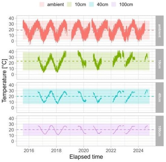
Figure 1.
Measured temperatures at each measurement depth. Dashed lines and shadow boxes represent the mean temperature at each depth and ambient conditions, with a range of ±2 standard deviations (SD). In this study, a range of ±2 SD from the mean was used to identify potential outliers, as it encompasses approximately 95.4% of the data in a normal distribution, providing a robust balance between sensitivity to anomalies and minimizing the misclassification of natural variability.
A distinct thermal gradient is observed, with temperature fluctuations decreasing with depth. The 100 cm depth shows appreciably smaller temperature variations compared to the 10 cm and 40 cm depths, indicating increased thermal stability in deeper soil layers. Seasonal temperature variations are evident across all depths, but their amplitude diminishes with increasing depth. Specifically, surface and shallow depths (10 and 40 cm) exhibit pronounced summer–winter temperature differences, while the 100 cm depth maintains a relatively stable temperature throughout the year, suggesting reduced influence from surface temperature changes.
3.1. Data Analysis
The results of long-term measurements of ambient and profile soil temperature are summarized in Table 1.

Table 1.
Summary statistics of temperature for each layer, including minimum (Min) and maximum (Max) values, median (Med), mean (Mean), standard deviation (SD), Range, Skewness, and Kurtosis.
An analysis of the temperature data revealed vertical thermal variations across four distinct layers. The ambient and shallow depth (10 cm) layers exhibited the largest temperature range, with fluctuations ranging from −6.4 to 42.4 °C. In contrast, deeper soil layers demonstrated a reduction in temperature variability. At a depth of 100 cm, temperatures stabilized within the range of 10.9 °C and 28.1 °C. The median temperatures were found to be consistent across the profile, ranging from 19.5 to 24.0 °C, with a peak recorded at 10 cm. The SD indicated variability within each layer, with the highest SD observed at ambient and 10 cm depths (both 8 °C), and the lowest SD recorded at 100 cm depth (5 °C), reflecting more stable temperatures at greater depths.
All depths exhibited slight negative skewness, with values ranging from −0.12 to −0.35, indicating distributions marginally shifted towards higher values. The kurtosis values were consistently negative across all depths, ranging from −0.71 to −1.50, indicating flatter, more spread-out distributions with fewer extreme values than would be expected in a normal distribution. The most pronounced uniform distribution was observed at Z = 100 cm (kurtosis = −1.50).
3.2. Modelling
Kasuda’s model (Equation (2)), grounded in heat conduction principles and outdoor temperature measurements, effectively characterizes soil temperature distribution across various depths and time periods. This approach enables robust analysis of soil temperature data, particularly valuable for soil permeability variations, harmonic temperature trend patterns, and studies investigating radon transport mechanisms. Our analysis employed both Kasuda’s ground temperature model (Equation (2)) and the sinusoidal ambient temperature model (Equation (1)), incorporating average values calculated from comprehensive measurements spanning a 9-year period across multiple soil depths and ambient conditions.
The results presented in Table 2 summarizes the fitted values of thermal diffusivity (), and peak temperature times (, ).
Table 2.
Thermal diffusivity (), ), and peak temperature times (, for ambient condition and different soil depths.
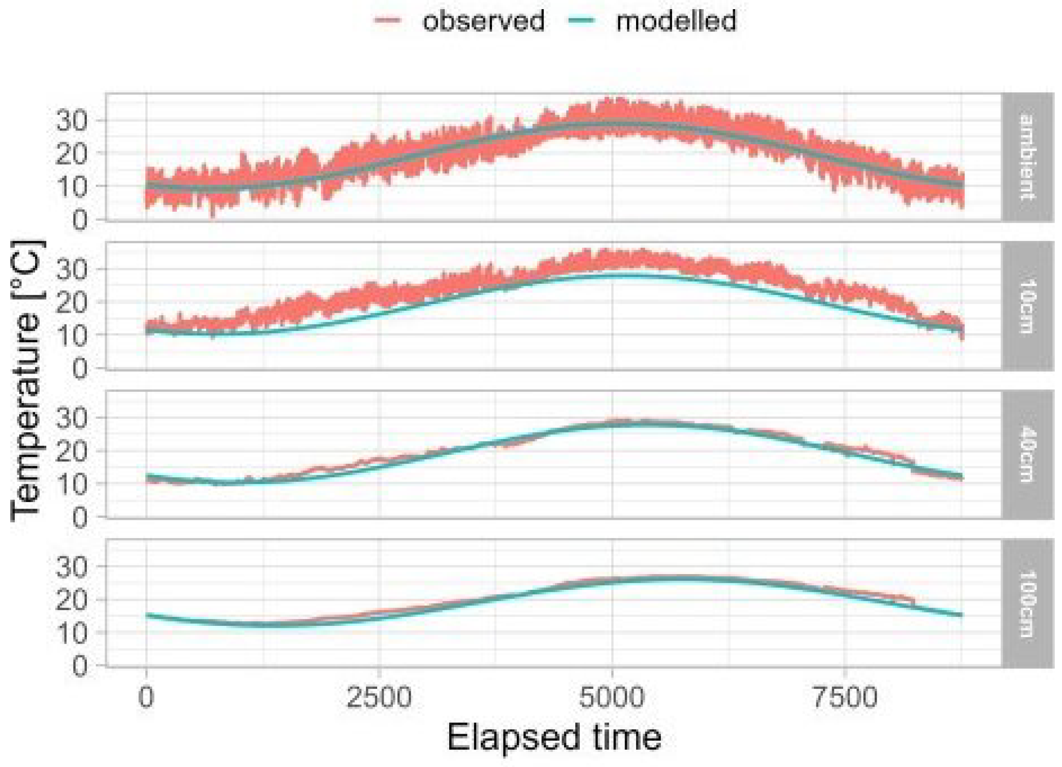
Measured and modelled temperature data are compared in Figure 2, with the corresponding fit parameters presented in Table 2.
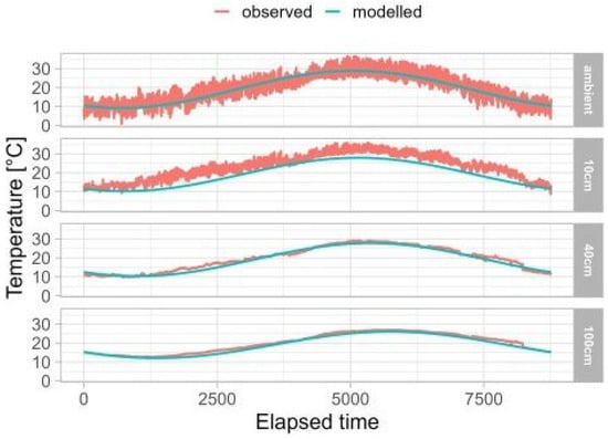
Figure 2.
Measured and modelled temperatures variations.
As shown, the measured ambient and 10 cm depth temperatures exhibit higher frequency fluctuations and generally higher peak values compared to deeper measurements. While the model captures the overall seasonal trend, it underestimates temperature fluctuations, particularly at the surface (10 cm). As depth increases, the agreement between modelled and measured temperatures improves, with the curves aligning more closely at 40 and 100 cm. This suggests that the model performs better at greater depths, where temperatures demonstrate increased stability, confirming the phenomenon of thermal buffering.
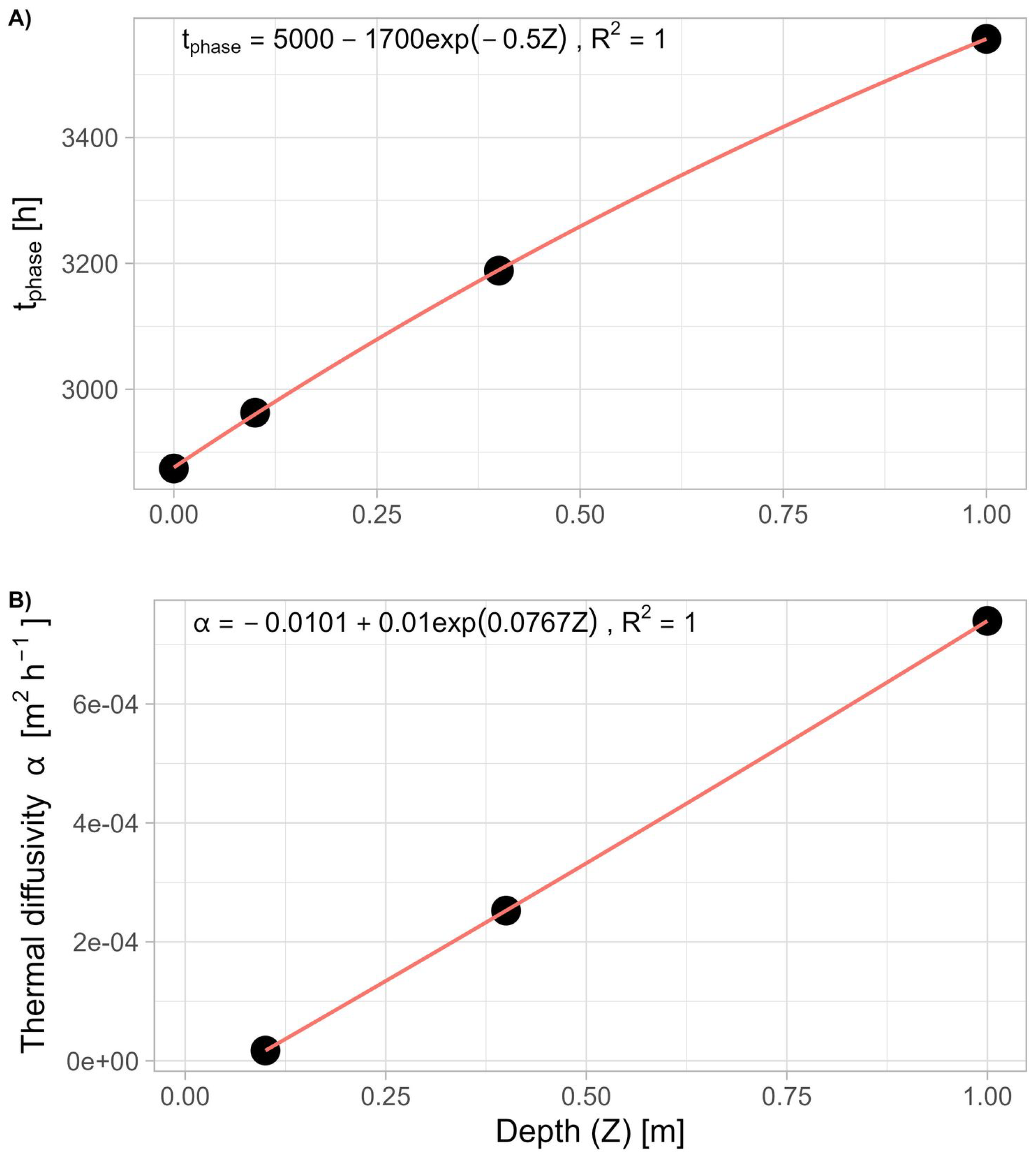
The observed increase in soil thermal diffusivity () and the phase parameter of sinusoidal temperature oscillation () with depth, as presented in Table 2 and Figure 3, reflects the combined effects of soil composition, structure, and moisture content.
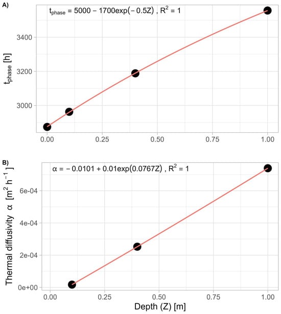
Figure 3.
(A) Phase shift () and (B) thermal diffusivity () as the functions of soil depth (Z). Modelled points (dots) are fitted with an exponential functions (line).
The relationship between and Z follows an exponential decay curve, i.e., . The parameter increases from about 2900 to 3500 h, as presented in Figure 3A, indicating that deeper soil layers take longer to reach their minimum and maximum values than shallower layers. This delay with depth can be attributed to the insulating properties of the soil.
Moreover, as seen in Figure 3B, the relationship between thermal diffusivity () and depth (Z) is exponential, given by . This indicates an increase from almost zero at the surface to approximately 7 × 10⁻⁴ m2 h−1 at a depth of 100 cm.
The observed reduction in thermal diffusivity at shallow depths can be attributed to several key factors. Increased porosity and organic matter content, along with the presence of air-filled pores, effectively reduce thermal conductivity. Air, being a poor conductor of heat, disrupts the transfer of thermal energy, while organic matter, with its lower thermal conductivity compared to mineral particles, further reduces heat transfer efficiency. Conversely, at greater depths, soil compaction and increased bulk density enhance particle-to-particle contact, facilitating more efficient heat conduction. While stabilized moisture content at these depths can contribute to consistent thermal properties, the reduction in organic matter and temperature fluctuations minimizes thermal resistance. These combined effects result in higher thermal diffusivity, as the soil’s ability to conduct heat improves with depth [18,19,20].
These findings emphasize the pivotal role of depth-dependent soil properties in modifying and delaying temperature variations, which has substantial implications for ground temperature modelling. The gradient in thermal diffusivity affects heat and mass transfer processes, including the transport of soil gases such as radon, influencing temperature-driven convective flows and diffusion rates within the soil matrix.
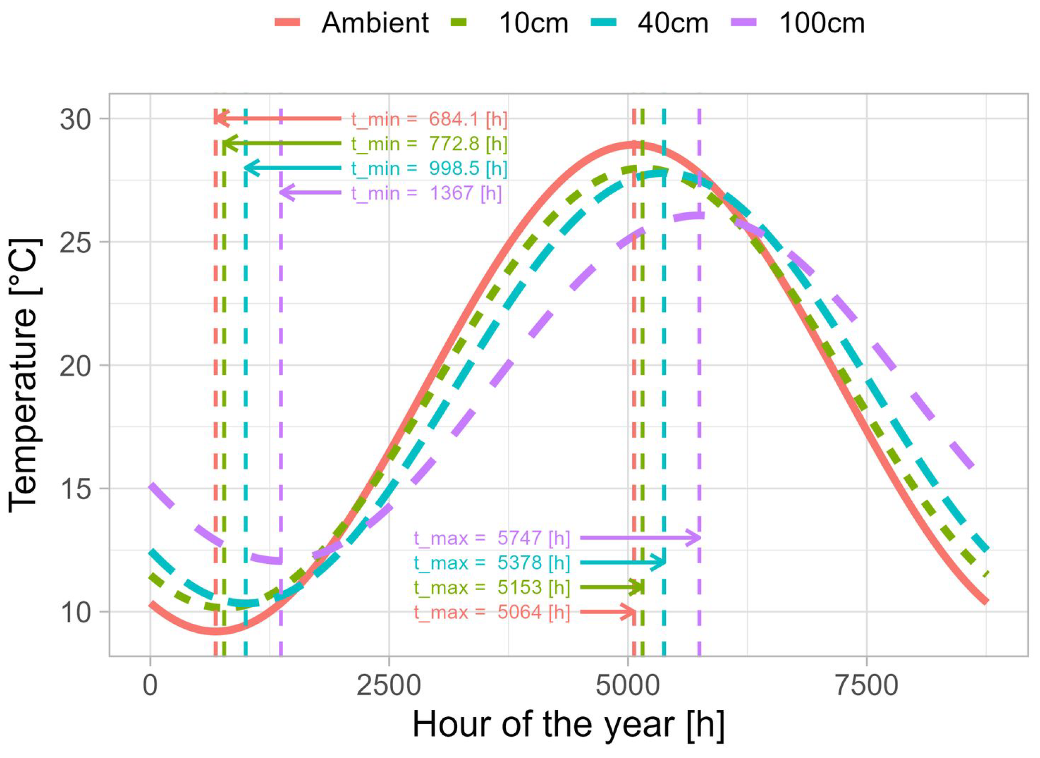
Figure 4 illustrates the modelled temperature variations at varying soil depths (10, 40, and 100 cm) and ambient conditions over the course of a year with the initial parameters of from Table 2.
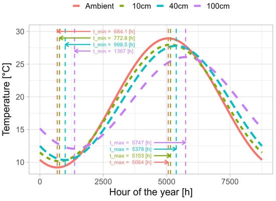
Figure 4.
Modelled temperature variations at different soil depths (10, 40, and 100 cm) and ambient conditions over a year, based on hourly averages from a 9-year measurement period with indication of and parameters.
The temperature curves demonstrate a sinusoidal pattern indicative of annual temperature cycles, with temperatures ranging from approximately 10 to 28 °C. The amplitude of temperature variation exhibits a decrease with depth.
A critical aspect of the graph is the time shift in minimum and maximum temperatures at varying depths. The analysis reveals that minimum temperatures progressively lag with increasing depth relative to the ambient minimal temperature measured at the end of January (≈ 683 h of the year ∼ 28 days). The delay is 88 h (≈3.5 days ∼end of January) at a depth of 10 cm, 311 h at 40 cm (≈13 days ∼middle of February), and 681 h at 100 cm (≈28 days ∼end of February). A similar trend is measured for maximum temperatures, which also exhibit a lag with a depth in relation to the maximum of ambient temperature at 5064 h of the year (≈end of July). The delay is 79 h at 10 cm (≈3.3 days ∼ beginning of August), 310 h at 40 cm (≈13 days ∼middle of August), and 680 h at 100 cm (≈28 days ∼end of August).
This phenomenon can be attributed to the principles of heat diffusion and the soil’s buffering effect on temperature fluctuations. Heat diffusion in soils follows Fourier’s law, where heat is transferred from areas of higher temperature to areas of lower temperature [21]. As heat penetrates deeper into the soil, it encounters resistance due to the soil’s thermal properties, such as thermal conductivity and diffusivity, as described earlier.
The soil’s buffering effect also plays a crucial role. Acting as a thermal buffer, the soil dampens temperature fluctuations as heat propagates through it. This buffering effect causes a delay and attenuation of temperature signals, with each successive layer contributing to the cumulative delay. As a result, temperature changes at greater depths are delayed relative to surface temperature changes, illustrating the combined effects of heat diffusion and soil buffering.
Figure 5 compares “Measured” soil temperature data with two different modelling approaches across three soil depths (10, 40, and 100 cm). Each data point represents the mean value for that specific hour calculated over the 9-year measurement period. The “Modelled” dataset was generated using Equation (2) with site-specific input parameters derived from Table 2. In contrast, the “ModelledDef” dataset was created using constant literature values of thermal diffusivity () for volcanic soil from previous studies [22,23] and parameter from our field measurements.
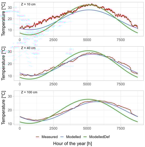
Figure 5.
Comparison of “Measured” soil temperature data with two modelled datasets at depths of 10, 40, and 100 cm. The “Modelled” line uses site-specific parameters from Table 2 in Equation (2), while “ModelledDef” uses literature values of for volcanic soil and constant based on our measurement.
Modelled and measured temperature oscillations show improved consistency with depth, indicating enhanced model performance in thermally stable, deeper soil layers. However, a timing discrepancy for minimum and maximum temperatures persists, particularly in deeper layers, when using constant and across all depths as presented by ModelledDef curve. This highlights the limitations of relying on generalized literature values for thermal diffusivity, as accurate soil temperature estimates necessitate incorporating site-specific parameters, including soil properties and depth-dependent variations. These findings emphasize the importance of precise temperature measurements for understanding complex soil temperature dynamics, especially near the surface, and their implications for radon transport.
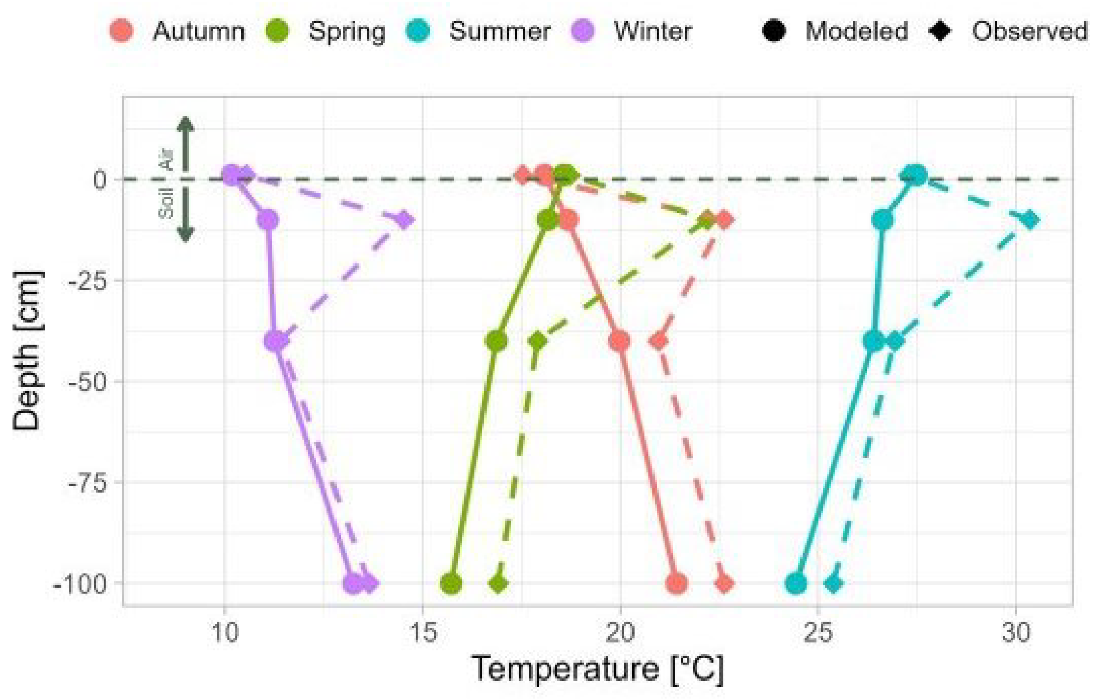
Figure 6 illustrates the seasonal variation of soil temperature profiles for both modelled and measured data with all layers (ambient and depth) for the average value of the entire period. The temperature profiles show clear seasonal stratification, with temperatures ranging from approximately 10 to 27 °C for the modelled data and from 11 to 32 °C for the measured data. Winter exhibits the coolest temperatures, while summer shows the warmest, with spring and autumn representing transitional periods. These findings reveal a distinct thermal gradient, demonstrating increasing thermal buffering with soil depth, which can be linked to an increase in thermal diffusivity.
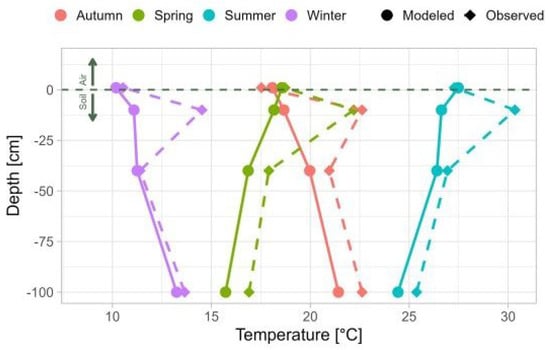
Figure 6.
Temperature variations across depth profiles for a continuous time span over mean value for different seasons (depth at 0 cm corresponds to ambient temperature measured at 100 cm above ground) for modelled (solid line) and measured (dashed line) data.
However, the comparison reveals noticeable differences between measured and modelled soil temperatures at a 10 cm depth across all seasons. These discrepancies are most pronounced in the transition seasons (spring and autumn), where the modelled temperatures consistently deviate from the measured values. This disparity may be attributable to either the influence of surface ambient conditions or potential sensor malfunctions.
The temperature profiles reveal interesting pattern similarities between winter–autumn and summer–spring pairs, demonstrating seasonal coupling in soil temperature dynamics (seasonal coupling refers to the synchronized patterns of change in soil temperature across different depths over the course of a year, driven primarily by seasonal variations in surface heat fluxes influenced by factors such as solar radiation, air temperature, and precipitation).
In the winter–autumn pair, both seasons show that the temperature increases with depth, being lowest at ground level. In the spring–summer pair, the temperature decreases with depth. Therefore, the largest temperature range was observed at 0 cm and the smallest at 100 cm. At 10 and 40 cm depths, the temperature ranges are comparable; however, in the spring–autumn pair, the difference increases with depth.
These seasonal couplings likely reflect the transition periods in annual soil temperature cycles, where winter–autumn represents the cooling phase and summer–spring the warming phase of the soil profile. The similarity in patterns despite different absolute temperatures indicates the consistent nature of heat transfer processes during these paired seasons, though the model captures these dynamics with varying degrees of accuracy across different depths.
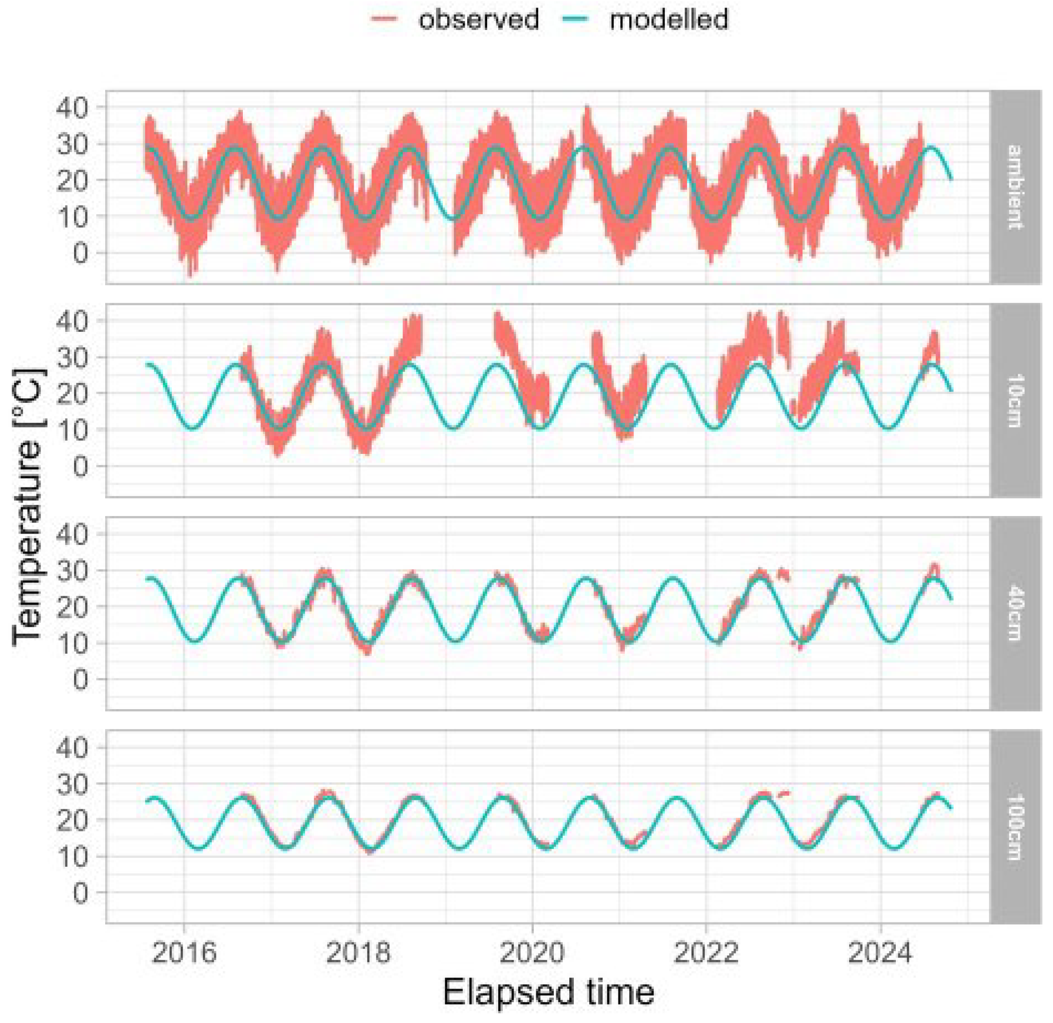
Using the data presented in Table 2, the modelling procedure was carried out and the results were then compared with the measured data throughout the entire measurement period (see Figure 7).
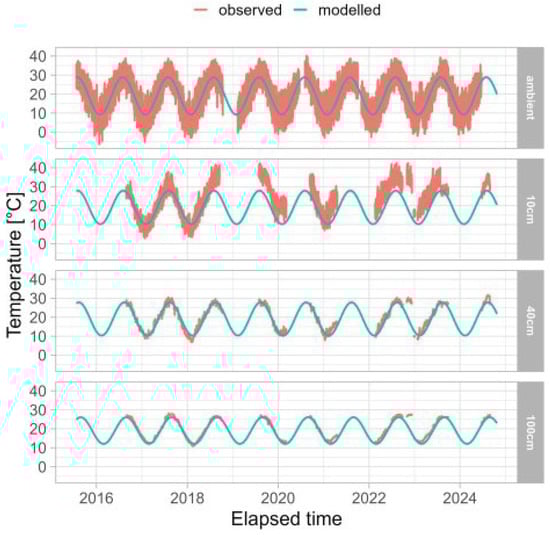
Figure 7.
Model application to whole measured data.
At the ambient level, the measured temperatures show considerable variability, with clear seasonal oscillations ranging from −6 to 40 °C. The model data exhibit comparable seasonal patterns but with reduced short-term variability, resulting in a more idealized sinusoidal curve in the range of 10 to 30 °C. Moving deeper into the soil profile, at depths of 10, 40, and 100 cm, several key patterns emerge. Initially, at a depth of 10 cm, the model initially underestimates the measured temperatures. While the modelled data closely match the observations during the first years of measurement, they show increasing divergence in subsequent years. This progressive deviation could be attributed to either changing environmental factors or gradual sensor deterioration. Secondly, the amplitude of the temperature fluctuations gradually decreases with depth, suggesting a dampening effect of the soil environment. At a depth of 100 cm, the temperature fluctuations are markedly less pronounced compared to the ambient measurements. Thirdly, a substantial enhancement in the congruence between measured and modelled temperatures and depth is evident, allowing for the capture of both diurnal and seasonal temperature fluctuations. Consistent annual temperature cycles, with summer peaks and winter troughs, are measured across all depths, though their amplitude diminishes with depth. This illustrates the soil’s thermal buffering capacity, where deeper layers exhibit increased stability and temperature patterns that more closely align with model expectations.
3.3. Temperature Model Application
The temperature model results offer a method to refine permeability calculations as expressed in Section 2.2. Standard methods rely on air suction measurements at a 50–100 cm depth, while temperature data is often collected at shallower levels. Our model estimates soil temperatures at greater depths using ambient temperature, minimizing the influence of soil profile temperature variations. For instance, a 10 °C difference between 10 and 100 cm depths in summer translates to an approximately 11% variation in calculated permeability (k). These variations increase uncertainty in Geogenic Radon Potential (GRP) assessments [9].
3.4. Limitations
While this study provides valuable insights into soil temperature dynamics and their implications for radon monitoring, several limitations and considerations merit discussion. First, our temperature measurements were affected by periodic equipment malfunctions and power outages, particularly evident in the data gaps of soil temperature between 2015 and 2024. These interruptions potentially impact our understanding of continuous temperature variations and their seasonal patterns. Second, the thermal diffusivity model, while effective at greater depths, shows notable discrepancies at shallow depths (particularly 10 cm), suggesting that our current approach may not fully capture the complex near-surface processes. These discrepancies could be attributed to various factors not incorporated in our model, including variations in soil moisture content, organic matter distribution, and local geological heterogeneity. The influence of precipitation and groundwater fluctuations on soil temperature profiles remains incompletely understood, as our study focused primarily on temperature measurements.
Additionally, while our findings are based on data from the Sakurajima volcano, the applicability of our model to other volcanic regions may be limited due to site-specific geological characteristics and local climate conditions. The exponential relationship we observed between thermal diffusivity and depth may vary in different volcanic settings, necessitating site-specific calibration.
Future research should address these limitations by incorporating continuous soil moisture measurements, analyzing the effects of precipitation patterns, and validating the model across different volcanic environments.
Furthermore, a more comprehensive investigation of sensor drift and long-term calibration stability would enhance the reliability of extended monitoring programs.
4. Conclusions
This study greatly advances our understanding of the temperature of soil in volcanic areas, providing a crucial foundation for future research. By conducting a thorough analysis of a nine-year temperature profile dataset from the Sakurajima volcano, we have attained novel insights that challenge conventional assumptions.
The findings demonstrate that thermal diffusivity varies exponentially with depth, rather than linearly, which has a substantial impact on soil temperature modelling.
In addition, the study identified optimal sensor placement depths (80–100 cm) for minimizing temperature-induced permeability variations, which can reach up to 11%.
Finally, the observed thermal buffering properties of soil, particularly the amplitude attenuation and temporal lag with depth, offer a practical framework for interpreting subsurface thermal behaviour.
The outcomes of this work suggest several promising directions for future studies:
- Soil temperature models can be refined by incorporating the observed depth-dependent thermal diffusivity, leading to more accurate predictions of subsurface thermal regimes.
- Furthermore, there is a need to investigate the complex interplay between soil moisture, meteorological parameters, and subsurface temperature variations.
- Exploration of the correlation between volcanic activity and measured temperature fluctuations is recommended, with the aim of improving our understanding of subsurface thermal responses to volcanic processes.
- The optimal sensor placement depths identified in this study should be utilized for enhanced monitoring of various subsurface processes, including but not limited to gas transport and heat flow.
- Addressing discrepancies observed at shallow depths (10 cm) by conducting targeted investigations into potential sensor malfunctions or localized soil condition effects to ensure the robustness of future datasets.
While the present study provides a valuable framework for understanding soil temperature dynamics, its implications extend beyond thermal analysis. The quantification of temperature-induced variations in permeability, particularly at a depth of 100 cm, provides critical insights for future studies involving gas transport, including radon. The findings of this study can be built upon to develop more accurate models and monitoring systems, which will lead to improved geohazard assessments and a deeper understanding of subsurface processes.
Author Contributions
Conceptualization, M.H., S.T. and M.J.; methodology, M.H.; formal analysis, M.J.; investigation, M.H., S.T., Y.O. and N.A.; writing—original draft preparation, M.J.; writing—review and editing, M.H., S.T., Y.O. and N.A.; visualization, M.J.; project administration, S.T.; funding acquisition, M.H., S.T., Y.O. and N.A. All authors have read and agreed to the published version of the manuscript.
Funding
This study was partially funded by the Environmental Radioactivity Network Center (ERAN) (Grant Number: P-24-43), the Japan Society for the Promotion of Science (JSPS) KAKENHI (Grant No. JP22H03010), and the “Project on Human Resource Development in Radiation Medicine for Responding to Complex Disasters (Theme 1: Dynamics of radioactive substances and air pollutants in the environment associated with earthquakes and volcanic activities and assessment of exposure and doses)”.
Institutional Review Board Statement
Not applicable.
Informed Consent Statement
Not applicable.
Data Availability Statement
The datasets analyzed in this study are available from the authors upon reasonable request, in accordance with the data sharing policies of QST and Hirosaki University. Data access may require a data sharing agreement.
Conflicts of Interest
The authors declare that there are no conflicts of interest.
References
- Sousa, J.J.; Liu, G.; Fan, J.; Perski, Z.; Steger, S.; Bai, S.; Wei, L.; Salvi, S.; Wang, Q.; Tu, J.; et al. Geohazards Monitoring and Assessment Using Multi-Source Earth Observation Techniques. Remote Sens. 2021, 13, 4269. [Google Scholar] [CrossRef]
- Wang, C.Y.; Manga, M. Changes in Tidal and Barometric Response of Groundwater during Earthquakes—A Review with Recommendations for Better Management of Groundwater Resources. Water 2023, 15, 1327. [Google Scholar] [CrossRef]
- Koizumi, N.; Sato, T.; Kitagawa, Y.; Ochi, T. Groundwater pressure changes and crustal deformation before and after the 2007 and 2014 eruptions of Mt. Ontake the Phreatic Eruption of Mt. Ontake Volcano in 2014 5. Volcanology. Earth Planets Space 2016, 68, 6–11. [Google Scholar] [CrossRef]
- Kotsarenko, A.; Yutsis, V.; Grimalsky, V.; Koshevaya, S.; Kotsarenko, Y. Anomalous temperature regimen in the near-surface soil layer of Tlamacas hill and its relation to activity of Popocatepetl Volcano, Mexico. BSGF-Earth Sci. Bull. 2020, 191, 3. [Google Scholar] [CrossRef]
- Yang, T.F.; Wen, H.Y.; Fu, C.C.; Lee, H.F.; Lan, T.F.; Chen, A.T.; Hong, W.L.; Lin, S.J.; Walia, V. Soil radon flux and concentrations in hydrothermal area of the Tatun Volcano Group, Northern Taiwan. Geochem. J. 2011, 45, 483–490. [Google Scholar] [CrossRef]
- Cigolini, C.; Poggi, P.; Ripepe, M.; Laiolo, M.; Ciamberlini, C.; Delle Donne, D.; Ulivieri, G.; Coppola, D.; Lacanna, G.; Marchetti, E.; et al. Radon surveys and real-time monitoring at Stromboli volcano: Influence of soil temperature, atmospheric pressure and tidal forces on 222Rn degassing. J. Volcanol. Geotherm. Res. 2009, 184, 381–388. [Google Scholar] [CrossRef]
- Hosoda, M.; Tokonami, S.; Suzuki, T.; Janik, M. Machine learning as a tool for analysing the impact of environmental parameters on the radon exhalation rate from soil. Radiat. Meas. 2020, 138, 106402. [Google Scholar] [CrossRef]
- Geological Survey of Japan AIST. Geological map of Japan, Kagoshima. Available online: https://www.gsj.jp/Map/EN/geology4-15.html (accessed on 1 April 2025).
- Janik, M.; Gomez, C.; Kodaira, S.; Grzadziel, D. Development of a new tool to simultaneously measure soil-gas permeability and CO2 concentration as important parameters for geogenic radon potential assessment. Environ. Monit. Assess. 2025, 197, 124. [Google Scholar] [CrossRef] [PubMed]
- ENVCO Global. WatchDog Soil Temperature Sensor. Available online: https://envcoglobal.com/catalog/water/water-quality-sensors/digital-sensors/digital-water-temperature-sensors/watchdog-soil/ (accessed on 1 April 2025).
- ENVCO Global. WatchDog 1000 Series Data Loggers. Available online: https://envcoglobal.com/catalog/agriculture/plant/disease-and-pests/barometric-1/ (accessed on 3 April 2025).
- Onset Computer Corporation. HOBO U30 USB Weather Station. Available online: https://www.onsetcomp.com/products/data-loggers/u30-nrc (accessed on 2 April 2025).
- Onset Computer Corporation. 12-Bit Temperature Smart Sensor. Available online: https://www.onsetcomp.com/products/sensors/s-tmb-m0xx (accessed on 2 April 2025).
- Florides, G.; Kalogirou, S. Annual ground temperature measurements at various depths. In Proceedings of the 8th REHVA World Congress, Clima, Lausanne, Switzerland, 9–12 October 2005; pp. 1–6. [Google Scholar]
- Florides, G.; Kalogirou, S. Measurements of Ground Temperature at Various Depths. In Proceedings of the 3rd International Conference on Sustainable Energy Technologies, University of Nottingham, Nottingham, UK, 27–29 June 2004. [Google Scholar]
- Kasuda, T.; Achenbach, P. Earth Temperature and Thermal Diffusivity at Selected Stations in the United States; Technical Report NBS REPORT 8972; National Berau of Standards: Gaithersburg, MD, USA, 1965. [Google Scholar]
- Boukhriss, M.; Zhani, K.; Ghribi, R. Study of thermophysical properties of a solar desalination system using solar energy. Desalin. Water Treat. 2013, 51, 1290–1295. [Google Scholar] [CrossRef]
- Ochsner, T. Rain or Shine: An Introduction to Soil Physical Properties and Processes; Oklahoma State University Libraries: Stillwater, OK, USA, 2019. [Google Scholar] [CrossRef]
- de Jong van Lier, Q.; Durigon, A. Soil thermal diffusivity estimated from data of soil temperature and single soil component properties. Revista Brasileira de Ciência do Solo 2013, 37, 106–112. [Google Scholar] [CrossRef]
- Xie, X.; Lu, Y.; Ren, T.; Horton, R. An empirical model for estimating soil thermal diffusivity from texture, bulk density, and degree of saturation. J. Hydrometeorol. 2018, 19, 445–457. [Google Scholar] [CrossRef]
- Romio, L.C.; Zimmer, T.; Bremm, T.; Buligon, L.; Herdies, D.L.; Roberti, D.R. Influence of Different Methods to Estimate the Soil Thermal Properties from Experimental Dataset. Land 2022, 11, 1960. [Google Scholar] [CrossRef]
- Kasubuchi, T. The effect of soil moisture on thermal properties in some typical Japanese upland soils. Soil Sci. Plant Nutr. 1975, 21, 107–112. [Google Scholar] [CrossRef]
- Suzuki, S.; Iiduka, K.; Sanada, A.; Ito, H.; Watanabe, F. Effects of thermal conductivity and diffusivity of a volcanic ash soil in central Ethiopian Rift Valley on soil temperatures. J. Arid. Land Stud. 2019, 29, 91–101. [Google Scholar] [CrossRef]


Disclaimer/Publisher’s Note: The statements, opinions and data contained in all publications are solely those of the individual author(s) and contributor(s) and not of MDPI and/or the editor(s). MDPI and/or the editor(s) disclaim responsibility for any injury to people or property resulting from any ideas, methods, instructions or products referred to in the content. |
© 2025 by the authors. Licensee MDPI, Basel, Switzerland. This article is an open access article distributed under the terms and conditions of the Creative Commons Attribution (CC BY) license (https://creativecommons.org/licenses/by/4.0/).