Article

The Use of River Flow Discharge and Sediment Load for Multi-Objective Calibration of SWAT Based on the Bayesian Inference

1
State Key Laboratory of Hydrology Water Resources and Hydraulic Engineering, Hohai University, Nanjing 210098, China
2
College of Hydrology and Water Resources, Hohai University, Nanjing 210098, China
3
Beijing Golden Water Information Technology and Services Co., Ltd., Beijing 100089, China
4
Institute of Geographical Sciences, Freie Universität Berlin, Malteserstraße 74-100, 12249 Berlin, Germany
*
Author to whom correspondence should be addressed.
Water 2018, 10(11), 1662; https://doi.org/10.3390/w10111662
Submission received: 25 September 2018 / Revised: 2 November 2018 / Accepted: 10 November 2018 / Published: 15 November 2018
(This article belongs to the Special Issue Watershed Hydrology, Erosion and Sediment Transport Processes )

Abstract

:
The soil and water assessment tool (SWAT) is widely used to quantify the spatial and temporal patterns of sediment loads for watershed-scale management of sediment and nonpoint-source pollutants. However few studies considered the trade-off between flow and sediment objectives during model calibration processes. This study proposes a new multi-objective calibration method that incorporates both flow and sediment observed information into a likelihood function based on the Bayesian inference. For comparison, two likelihood functions, i.e., the Nash–Sutcliffe efficiency coefficient (NSE) approach that assumes model residuals follow the Gaussian distribution, and the BC-GED approach that assumes model residuals after Box–Cox transformation (BC) follow the generalized error distribution (GED), are applied for calibrating the flow and sediment parameters of SWAT with the water balance model and the variable source area concept (SWAT-WB-VSA) in the Baocun watershed, Eastern China. Compared with the single-objective method, the multi-objective approach improves the performance of sediment simulations without significantly impairing the performance of flow simulations, and reduces the uncertainty of flow parameters, especially flow concentration parameters. With the NSE approach, SWAT-WB-VSA captures extreme flood events well, but fails to mimic low values of river discharge and sediment load, possibly because the NSE approach is an informal likelihood function, and puts greater emphasis on high values. By contrast, the BC-GED approach approximates a formal likelihood function, and balances consideration of the high- and low- values. As a result, inferred results of the BC-GED method are more reasonable and consistent with the field survey results and previous related-studies. This method even discriminates the nonerodible characteristic of main channels.

1. Introduction

The soil and water assessment tool (SWAT) as a semidistribution hydrologic model is popularly used to assess water resource and soil erosion problems in the globe [1,2]. Soil erosion from each hydrologic response unit (HRU) in SWAT is simulated by a modified universal soil loss equation (MUSLE) [3], and the simplified Bagnold equation [4,5] is used as a kind of sediment routing approaches to simulate the sediment transport in the channel network. Obviously, sediment loads in the watershed outlet are closely related to the surface runoff of slopes and the flow velocity of channels.
Most previous studies calibrated the SWAT model using flow or sediment objective following the calibration procedure of first flow then sediment [6,7]. This calibration procedure did not take into full account the trade-off information between flow and sediment objectives [8], and could affect the performance of sediment simulations and increase the uncertainty of model parameters [9]. By contrast, the multi-objective calibration method may have advantages in improvement of the robustness, calibration efficiency, and model certainty [10].
The simplest way to solve a multi-objective problem is to convert the multiple objectives into a single objective, e.g., the weighted sum principle where objectives are multiplied with user-defined weights and then added together to form a single objective [11,12]. In this method, however, it is equivocal to choose user-defined weights [10]. Alternatively, evolutionary algorithms to search the “Pareto front”, i.e., a set of special points where we cannot further improve one objective without impairing other objective, are utilized for calibrating parameters of SWAT with both flow and sediment objectives [8,13].
Many Pareto-based multi-objective calibration algorithms have been developed such as the multi-objective complex evolution (MOCOM) method [9], the multi-objective shuffled complex evolution metropolis algorithm (MOSCEM) [14], the nondominated sorting genetic algorithm (NSGA-II) [15], and the multi-algorithm genetically adaptive multi-objective method (AMALGAM) [16]. However, there are still some disadvantages in using these approaches: (1) they can only obtain the “Pareto front”, rather than best fit results, so it still needs to convert the multi-objective values into a single value using the weighted sum principle for determination of the optimum solution [17]; (2) they are usually complex and time-consuming [10]; (3) they are difficult to estimate the parameter uncertainty because most parameter uncertainty analysis methods (such as Markov Chain Monte Carlo (MCMC) and Generalised Likelihood Uncertainty Estimation (GLUE)) are based on a single objective [18,19,20].
Reichert and Schuwirth [18] developed a scheme for linking statistical bias description to multi-objective model calibration. In this frame, all model residuals are lumped into a single additive residual term that is measured by a likelihood function under the assumption that the residuals of different objectives are independent of each other. This scheme avoids the trouble of choosing weights and can combine with the Bayesian approach to analyze parameter uncertainty. However, it is so complex that it lacks practicability, e.g., only the Gaussian error distribution is simply demonstrated by Reichert and Schuwirth [18] and Tang et al. [21].
This study tried to build a new multi-objective calibration approach based on the Bayesian inference, and analyze the effect of different likelihood functions on model calibration results. We first established a method to convert flow and sediment objectives into a likelihood function. Then, two likelihood functions of the NSE and BC-GED are used as the optimization objective functions to calibrate flow and sediment parameters of SWAT with the water balance model and the variable source area concept (SWAT-WB-VSA) in the Baocun watershed, Eastern China [2]. The Nash–Sutcliffe efficiency coefficient (NSE) approach assumes that errors between observed and simulated outcomes follow the Gaussian distribution [22], and the BC-GED approach first utilizes the Box–Cox transformation (BC) to remove the heteroscedasticity of model residuals and then assumes that model residuals after BC transformation follow the generalized error distribution (GED) [23]. Finally, the Bayesian inference results (e.g., posterior distribution of parameter set) of the NSE approach are compared with that of the BC-GED method for studying the effect of likelihood functions.

2. Study Area

2.1. Baocun Watershed

The Baocun watershed (86.7 km2) is a rural watershed located in the eastern Jiaodong Peninsula in China (Figure 1), where the average watershed slope is about 8.2‰. The watershed lies in the West Pacific Ocean extratropical monsoonal region with 70% of rain falling between June and September and a great variability of interannual precipitation. During the record period beginning in 1956, the maximum annual precipitation was observed in 2003 with 1219.7 mm, and the minimum occurred in 1999 with 383.7 mm. The average annual precipitation and the potential evapotranspiration were 805.6 and 899.0 mm, respectively. The average monthly temperature ranged from −0.8 °C in January to 24.4 °C in August. It has been proved that SWAT-WB-VSA was appropriate for the simulation of river discharges in the Baocun watershed by Cheng et al. [2].

2.2. Model Input Data

The digital elevation model (DEM) with 30 m resolution was produced by the natural neighbor interpolation method from the 1:10,000 scale topographic map (Figure 1b) provided by Hydrology and Water Resource Survey Bureau of Weihai. The watershed was divided into 7 sub-basins according to the river system (Figure 1b). The map of 10 equal area topographic classes is shown in Figure 2a, where the value of TI is the averaged TI across each topographic index class.
The resolution of soil type map from the Harmonized World Soil Database [24] is about 1 km, which is too coarse for our study. Therefore, we reclassified soil types according to TI values because of the uniform geological condition within a small mountain watershed. According to the Harmonized World Soil Database [24], the area proportions of regosols, luvisols, and fluvisols are about 50%, 30%, and 20%, respectively, in the Baocun watershed. So, TI values within the ranges of 3.2–7.5, 7.5–9.5, and 9.5–24.3 respectively correspond to regosols, luvisols, and fluvisols (Figure 2b), which account for 50%, 30%, and 20% of total area. The soil physical properties are presented in Table 1. In this table, the USLE_K value was estimated by an equation proposed by Williams [3]. Results show that the value of USLE_K1 (Regosols) is greater than that of USLE_K2 (Luvisols), and greater than that of USLE_K3 (Fluvisols).
The land use is only agriculture. However, crops cyclically vary because of the crop rotation method with farming, which occurs three times in every two years. The average annual land use map was charted to overcome the problem of land utilization change. The detailed steps are that we firstly extracted the fixed land use from the 1:10,000 scale topographic map, such as water body, forest, and residential area, and then randomly filled the rest of the area by peanut, winter wheat and corn with the proportion of 0.25, 0.5, and 0.25, respectively, according to the growth time of crops. The average annual land use map is shown in Figure 2c.
Meteorological data include daily maximum and minimum air temperatures, wind speed, relative humidity and solar radiation which were collected from three national weather stations (Weihai, Chengshantou, and Shidao, Figure 1a) and provided by China Meteorological Administration. The precipitation data were from four rainfall gauges inside Baocun watershed (Figure 1b). The potential evapotranspiration (PET) value was measured by E601 pan evaporation equipment at the Baocun hydrometric station (Figure 1b).
Daily river discharge data within the period of 1993–1999 and daily sediment load data within the flood period (from June to September) at the Baocun hydrometric station (Figure 1b) are used as observed outcomes for the Bayesian inference. The model calculation periods are from 1990 to 1999, where the period from 1990 to 1992 is used for model warm-up. The length of model warm-up period had been considered the balance of the effect of initial conditions on model simulations and the model elapsed time.
The hydrological data were provided by the Hydrology and Water Resource Survey Bureau of Weihai, which were collected strictly according to codes for liquid flow and suspended load measurement in open channels published by Ministry of Water Resources of China [25,26]. The Baocun hydrometric station belongs to the third type station with the relatively low accuracy [25,26]. The specifications state that the accuracy associated with the stage-discharge rating curves in the Baocun station should be greater than 89%. The flow velocity was measured by the propeller or wheel-cup type current meter (with the accuracy greater than 97%) that was transported to the open channel along the cableway using a motorized winch. And the water level was observed by the water level gauges with the absolute error less than 0.5 cm.
Sediment samples were collected by the grab method, of which the frequency was about once per hour usually and higher than that sometimes for covering the flood processes. The repeat sample method was used as a quality control approach to ensure accurate sediment concentrations that were measured by the oven-dry method. The instantaneous sediment load was calculated using the instantaneous cross-section mean sediment concentration (that was estimated by the sediment concentration at a fixed measuring point versus the cross-section mean sediment concentration curves) to multiply the instantaneous river discharge, of which the accuracy was greater than 80%. The daily sediment load is the average value of instantaneous sediment loads.

3. Methods

3.1. SWAT-WB-VSA Model

White et al. [27] incorporated a water balance model (WB) with spatial adjustments by using the soil wetness index to replace the SCS-CN rainfall–runoff method in SWAT, and developed a new SWAT model termed SWAT-WB. SWAT-WB was further improved by establishing a relationship between the effective depth of soil profile in WB and the topographic index, which represents the variable source area (VSA) concept (termed as SWAT-WB-VSA) [2]. SWAT-WB-VSA improved the surface runoff generation approach without changing others, such as estimation methods of the groundwater, channel routing, and sediment.

3.1.1. Surface Runoff Generation

In every Hydrologic Response Unit (HRU) of SWAT-WB-VSA, runoff occurs only when the precipitation amount is larger than the available soil moisture storage (τ):
Q surf = { R d a y τ R d a y > τ 0 others
where Qsurf is the overland flow (mm) and Rday is the daily rainfall (mm).
τ is also termed as the saturation deficit in the soil profile:
τ = E D C × ε θ
where EDC is the effective part of soil profile (unitless, ranging from 0 to 1), ε is the total soil porosity (mm) and θ is the volumetric soil moisture for each day (mm).
To express the spatial variation of rainfall–runoff mechanism influenced by the topography in addition to the soil, the soil type map is substituted by a soil topographic index map, which combines the soil type map with the topographic index map (TI, and TI = ln(A/tanβ), where A is the upslope contributing area and tanβ is the slope). Each topographic index class has its own parameter of EDC (i.e., EDCi). SWAT-WB-VSA assumes a linear relation between EDCi for each topographic class and TIi based on TOPMDODEL concept [2]:
E D C i = { 1 T I i T I ¯ × ( 1 E D C ) T I i T I ¯ × ( 1 E D C ) < 1 0 others
where T I ¯ and EDC are the catchment average TIi and EDCi, respectively.

3.1.2. Sediment

Sediment simulation involves two aspects: erosion of soil particles from slopes and sediment transport in the channel network. MUSLE model is used to estimate the soil erosion from HRUs [3]:
s e d = 11.8 × ( Q surf × q peak × a r e a HRU ) 0.56 × K × C × P × L S × C F R G
where sed is the sediment yield (ton), q peak is the peak runoff rate (m3/s), a r e a HRU is the area of HRU (ha), K is the soil erodibility factor (USLE_K; 0.013 ton m2 h/(m3 ton cm)), C is the cover and management factor (unitless), P is the support practice factor (unitless), LS is the topographic factor (unitless), and CFRG is the coarse fragment factor (unitless).
q peak is equal to:
q peak = a d j pkr × Q surf × a r e a HRU 3.6 × t conc
where a d j pkr is the peak rate adjustment factor (ADJ_PKR, unitless) and tconc is the time of concentration from HRU to the sub-basin outlet (h), which includes the overland flow time (tov; h) and the tributary channel flow time (tch; h), which are all estimated using Manning’s equations:
t conc = t ov + t ch
t ov = L slp 0.6 × n ov 0.6 18 × s l p 0.3
t ch = 0.62 × L ch × n ch 0.75 a r e a 0.125 × s l p ch 0.375
where Lslp is the subbasin slope length (m), slp is the average slope in the subbasin (unitless), nov is the Manning’s roughness coefficient for subbasin slope (OV_N; unitless), Lch is the channel length from the most distant point to the subbasin outlet (km), nch is the Manning’s roughness coefficient for the tributary channel (CH_N1; unitless), area is the subbasin area (ha), and slpch is the channel slope (unitless).
The amount of sediment released to the main channel (sed′ i.e., sediment lag in the surface runoff; ton) is calculated by an exponential decay model:
s e d = ( s e d + s e d stor , i 1 ) × ( 1 exp ( s u r l a g / t conc ) )
where sedstor,i−1 is the sediment stored or lagged from the previous day (ton), and surlag is the surface runoff lag coefficient (SURLAG; unitless).
The simplified Bagnold equation is used to estimate the sediment transport capacity in main channels (sedmx; ton):
s e d mx = s p c o n × ( p r f × q c h / A ch ) s p e x p × q ch
where spcon is the coefficient defined by users (SPCON; unitless), prf is the channel peak rate adjustment factor (PRF; unitless), Ach is the cross-sectional area of flow in channel (m2), spexp is the exponent defined by users (SPEXP; unitless), and q ch is the average rate of flow (m3/s), calculated by the Manning’s equation:
q ch = A ch × R ch 2 / 3 × s l p ch 1 / 2 / n ch
where Rch is the hydraulic radius for a given depth of flow (m), and nch is Manning’s roughness coefficient for the main channel (CH_N2; unitless).
If the sediment load from upstream is greater than sedmx, i.e., sed′ > sedmx, the deposition will be the dominant process in the reach segment and the sediment deposition amount (seddep; ton) is:
s e d dep = s e d s e d mx
If the sediment load from upstream is less than sedmx, the degradation will be the dominant process in the reach segment and the sediment degradation amount (seddeg; ton) is:
s e d deg = ( s e d mx s e d ) C H EROD C CH
where CHEROD is the channel erodibility factor (CH_EROD; unitless) and CCH is the channel cover factor (unitless).

3.2. Model Calibration

The Bayesian theorem describes the relationship between the conditional distribution for model parameter set (θ) given observed outcomes (obs) and the joint distribution of θ and obs. The Bayesian theorem states:
π ( θ | o b s ) = π ( θ ) l ( θ | o b s ) π ( θ ) l ( θ | o b s ) d θ π ( θ ) l ( θ | o b s )
where π(θ) is the prior distributions for parameter set (θ), l(θ|obs) is the likelihood function, π ( θ ) l ( θ | o b s ) d θ is the marginal likelihood (that usually sets to unknown constant), and π(θ|obs) is the posterior distribution for θ given obs.
However, it is difficult to obtain the analytical solution and compute the numerical solution in Equation (14) because of the unknown formulation of hydrologic models and too many model parameters [28]. The Markov Chain Monte Carlo (MCMC) scheme provides a simple and effective way around the computational efforts for estimation of the posterior distribution in Equation (14). The aim of MCMC scheme is to randomly generate samples of the parameter set based on constructing a Markov chain that has the posterior distribution as its equilibrium distribution [29]. By contrast, the Differential Evolution Adaptive Metropolis (DREAM) MCMC sampling is superior to other adaptive MCMC sampling approaches in the presence of high-dimensionality and multimodality optimization problems, because the DREAM scheme follows up on the Shuffled Complex Evolution Metropolis (SCEM-UA) global optimization algorithm, runs multiple different chains simultaneously for global exploration, and maintains detailed balance condition [30]. In this study, we selected 8 parallel chains and a total of 40,000 model evaluations for DREAM algorithm parameterization on the R platform, and ran them on the “Soroban” High-Performance Computing System at Freie Universität Berlin.
For SWAT-WB-VSA model in this study, 25 key parameters with 17 flow parameters and 8 sediment parameters are selected to be identified by model calibration (Table 2) according to previous studies with sensitivity analysis results [2,7,31,32]. The min and max ranges of model parameters in this study are referred to advisable parameter boundaries provided by previous studies [2,7,31,33]. Please note that the unit of soil erodibility factor (USLE_K) is 0.013 ton m2 h/(m3 ton cm) (Table 1).
There are 4 flow parameters in Equations (7)–(9) and (11) (i.e., OV_N, SURLAG, CH_N1 and CH_N2) that directly influence sediment loads. And the amount of overland flow (Qsurf) significantly affects the yield of soil erosion from slopes (Equations (4) and (5)).

3.3. Transformation of Flow and Sediment Objectives to a Likelihood Function

The likelihood function of a set of model parameter values (θ) given observed outcomes (obs) is equal to the joint probability of observed outcomes given the parameter values. Assuming errors ( e i ) between observed and simulated flow follow the distribution of p( e i , flow ), the logarithmic likelihood function of flow can be expressed as [22,23]:
l ( θ | o b s flow ) = ln [ i = 1 n p ( e i , flow | θ ) ] = 1 n ln [ p ( e i , flow | θ ) ]
where e i , flow is the error between observed and simulated river discharge (i.e., flow) at the time step i, and n is the length of flow time series.
Similarly, if errors ( e i ) of sediment loads follow the distribution of p′( e i , sed ), the logarithmic likelihood function of sediment is:
l ( θ | o b s sed ) = ln [ i = 1 m p ( e i , sed | θ ) ] = 1 m ln [ p ( e i , sed | θ ) ]
where e i , sed is the error between observed and simulated sediment load at the time step i, and m is the length of sediment time series.
If model residuals of sediment ( e i , sed ) are independent on that of flow ( e i , flow ), the logarithmic likelihood function of flow and sediment (i.e., the joint probability of flow and sediment residuals) can be described as:
l ( θ | o b s ) = l ( θ | o b s flow ) + l ( θ | o b s sed ) = 1 n ln [ p ( e i , flow | θ ) ] + 1 m ln [ p ( e i , sed | θ ) ]
Note that the sediment loads and the river discharges are two different hydrological processes. Although the river discharges affect the sediment loads, there are many other factors that influence the sediment amount, e.g., topography, soil textures, land covers and human activities. Therefore, it is appropriate to assume that the sediment and flow residuals are independent. The independent assumption will be tested in our case study.

3.3.1. Case with NSE

The Nash–Sutcliffe efficiency coefficient (Nash and Sutcliffe [34]; NSE) is widely used as the efficiency criterion for hydrologic modeling assessment:
NSE = 1 1 n ( s i m i o b s i ) 2 1 n ( o b s i o b s ¯ ) 2
where obsi and simi are the observed and simulated outcomes at the time step i, respectively, and o b s ¯ is the mean observed outcomes.
NSE is dimensionless and ranges from minus infinity to 1. If NSE is equal to 1, the model-simulated results perfectly match the observations; if NSE is less than 0, the hydrologic model is not better than a predictor using the mean of observations. It has been proved that NSE is equivalent to a kind of likelihood function with the assumption that residuals follow a Gaussian distribution with zero mean [22]. Substituting NSE into Equation (17), the logarithmic likelihood function changes to:
l ( θ | o b s ) = n 2 ln ( 2 π ε n 1 n σ obs , flow 2 ) n 2 ln ( 1 NSE flow ) m 2 ln ( 2 π ε m 1 m σ obs , sed 2 ) m 2 ln ( 1 NSE sed )
where ε is the base of natural logarithm ≈ 2.718, σ obs , flow and σ obs , sed are the standard deviation of the observed flow and sediment, respectively, and NSEflow and NSEsed are the Nash–Sutcliffe efficiency coefficient of flow and sediment, respectively.

3.3.2. Case with BC-GED

A general distance-based goodness-of-fit indictor (BC-GED) was proposed by Cheng et al. [23]:
BC-GED = Γ ( 1 / β ) β ε β 1 n | o b s i λ s i m i λ | β n × | λ | β β
where Γ(x) is the gamma function evaluated at x, β is the power (i.e., kurtosis coefficient) of model residual (β > 0), and λ is the Box–Cox transformation parameter (BC).
The currently used distance-based goodness-of-fit indicators (e.g., mean squared error (MSE) and square-root transformed MSE (RTMSE)) can be unified by BC-GED that assumes the model residuals after Box–Cox (BC) transformation follow the generalized error distribution (GED) with zero-mean. BC-GED has two parameters: the BC transformation parameter λ and the kurtosis coefficient β. β can be estimated by minimization of the BC-GED value. And λ can be calculated by the following constraint which minimizes the variance of time series of model residuals for removing the heteroscedasticity of model residuals:
min ( variance ( e i ) ) = 1 n 1 1 n ( o b s i λ s i m i λ λ μ ) 2 | m i n
where μ is the mean of model residuals after BC transformation.
Substituting BC-GED into Equation (17), the logarithmic likelihood function changes to:
l ( θ | o b s ) = n ln [ 2 BC-GED flow ] m ln [ 2 BC-GED sed ]
where BC-GEDflow and BC-GEDsed are the BC-GED values of flow and sediment, respectively.

4. Results

4.1. NSE Approach

The NSE approach first calculates NSE values of flow (NSEflow) and sediment (NSEsed) after running SWAT-WB-VSA model with parameter set (θ), and then substitutes NSE values into Equation (19) to calculate the likelihood function value at each MCMC iteration.
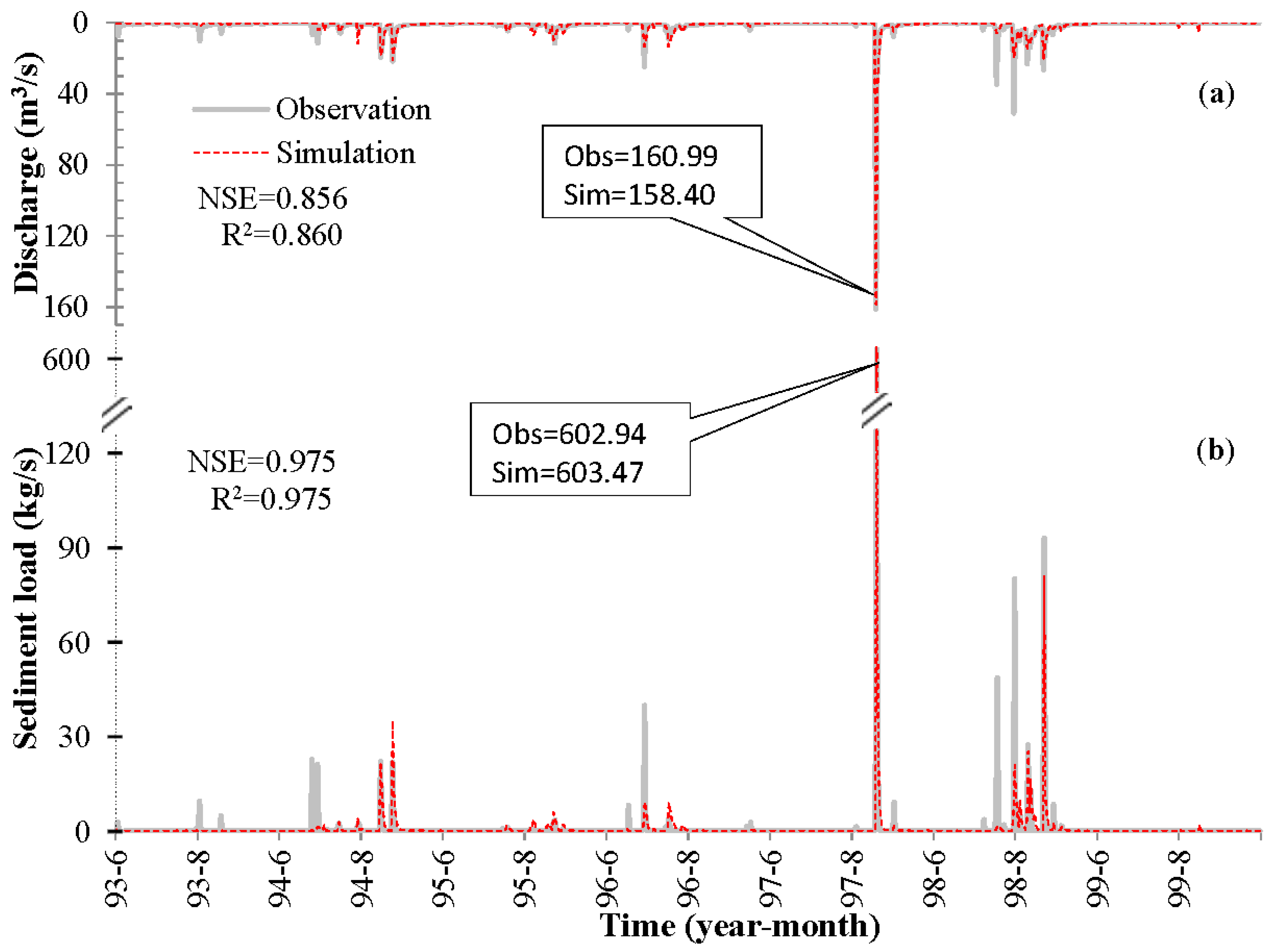
The best simulation results corresponding to the maximum likelihood function value in Equation (19) is shown in Figure 3. This figure shows that, with the NSE approach, the hydrologic model mimics the observed river discharges and sediment loads well, which reproduces most major flood events, especially the large flow discharges and sediment loads. Surprisingly, the NSE value of sediment is higher than that of flow in Figure 3. However, the NSE value of sediment decreases to 0.577 as the largest value of sediment loads in 1997 is ignored. It confirms that the criterion of the NSE puts great emphasis on high value [23].
The amount of flow discharge and sediment load during flood period from 1993 to 1999 in Table 3 is shown that in high flow years (such as 1994, and 1996–1998), SWAT-WB-VSA with the NSE approach can maintain small relative errors between observations and simulations of flow/sediment. In low flow years, however, the model yields a large relative error especially of sediment. For example, in 1995 and 1999, the model obviously over-estimates the sediment loads, but under-estimates in 1993.
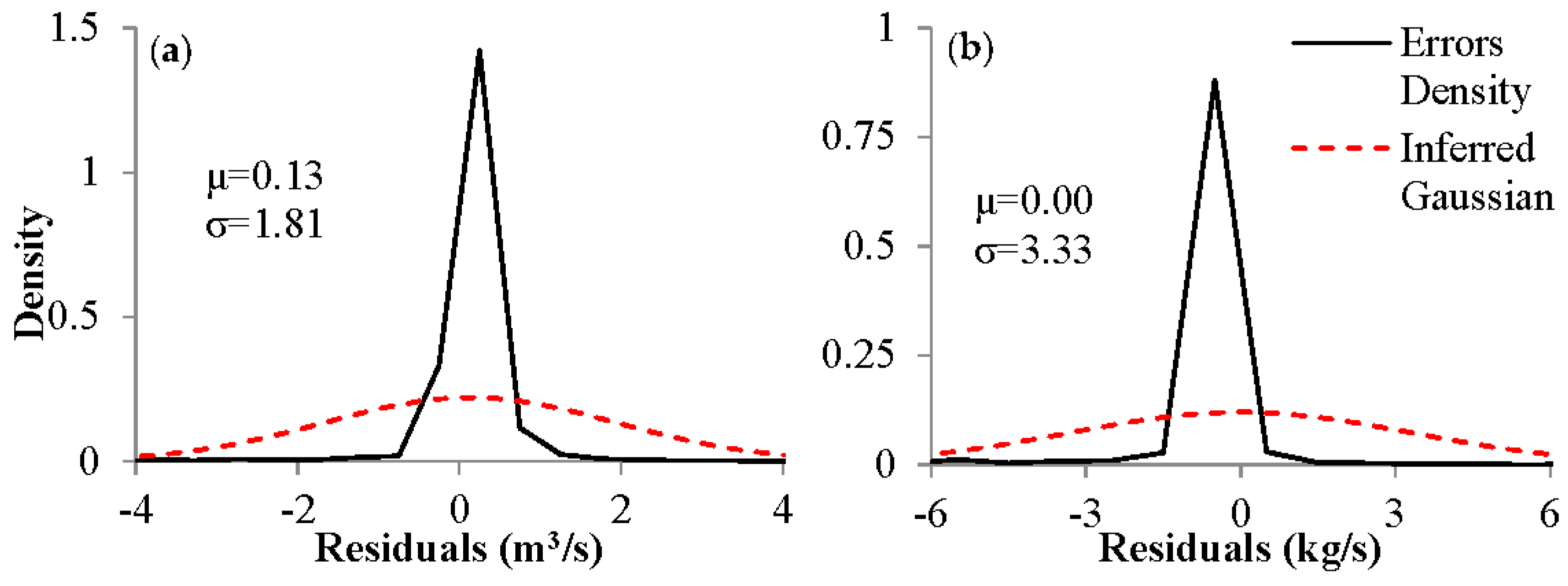
According to Equation (19), the NSE approach assumes that residuals follow the Gaussian distribution, of which the assumption for flow and sediment residuals is inspected in Figure 4. In this figure, “μ” and “σ” are the mean and standard deviation of model residuals, respectively. And the empirical probability density is estimated by the histogram of model residuals. Figure 4 shows that error histograms of both flow and sediment are substantially different from their assumed Gaussian distribution with zero-mean. This violation demonstrates that the NSE approach cannot guarantee that model residuals of both flow and sediment fulfill their statistical assumptions. Therefore, the NSE approach belongs to an informal likelihood function.
Computed by SWAT-WB-VSA with the optimum parameter set, the average annual components of simulated flow and sediment are shown in Table 4. For evaluating the effect of multi-objective method on simulated runoff, Table 4 also includes the average annual runoff components inferred by the single-objective (i.e., flow discharge) method [22]. This table shows that for the NSE approach the runoff components are nearly no difference between multi- and single- response calibration method, where the main runoff components are groundwater return flow and the main pathway of groundwater loss is revaporization (i.e., evaporation).
In Table 4 for sediment, “Total slope erosion” represents the amount of soil erosion from slopes/HRUs, and “Total river erosion” represents the amount of soil erosion from channels, where the positive value means erosion and the negative value means deposition. The main channels are rivers 5, 6 and 7 shown in Figure 1b, where the rivers 5 and 6 belong to the second level river and river 7 belongs to the third level river according to the Strahler stream order method [35]. The sediment loads inferred by the NSE approach demonstrate that the main channels in the Baocun watershed are all erosional and were actively incising into their beds over the period of simulation. And more than 36% of sediment loads at the watershed outlet come from main channels.
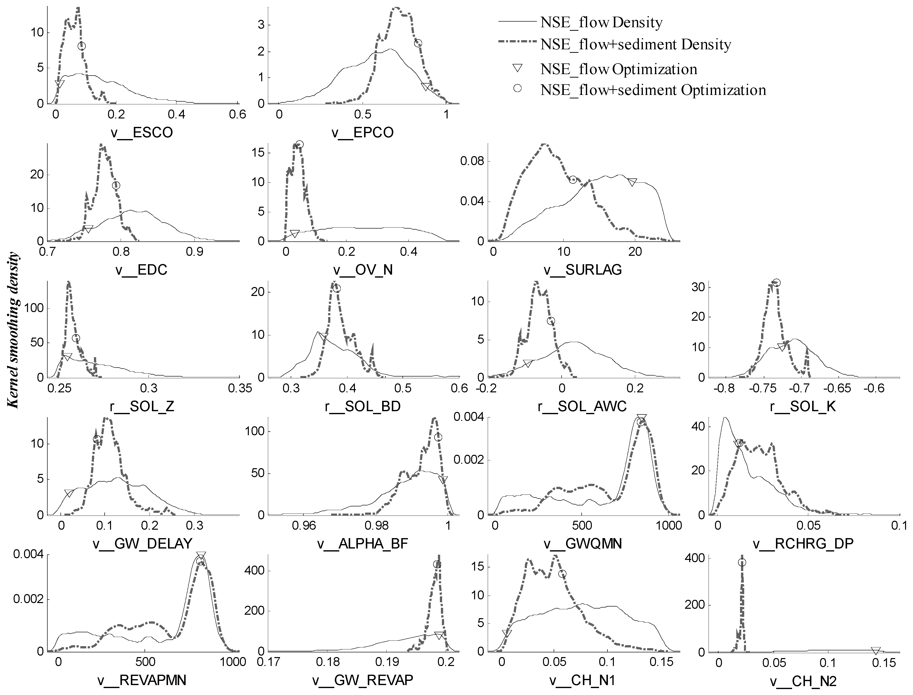
Targeted on flow parameters, Figure 5 shows the posterior parameter distribution (after kernel smoothing) and optimal value of flow parameters estimated by the multi- and single-objective NSE approaches. Some optimal flow parameter values of the multi-objective NSE approach, such as soil property parameters and groundwater storage and movement parameters (e.g., ALPHA_BF, GWQMN and RCHRG_DP), are similar to those of the single-objective method, which is in agreement with the results in Table 3 where average annual runoff components of both methods are nearly the same, possibly because these parameters have the least effect on sediment erosion. However, the posterior distribution of most flow parameters estimated by the multi-objective NSE approach are sharper than those estimated by the single-objective method, especially the Manning’s coefficients of sloping surface (OV_N) and main channel (CH_N2). Above results illustrate that the multi-objective approach by combining flow with sediment information would reduce the parameter searching range and thus increase the certainty of parameter optimization.
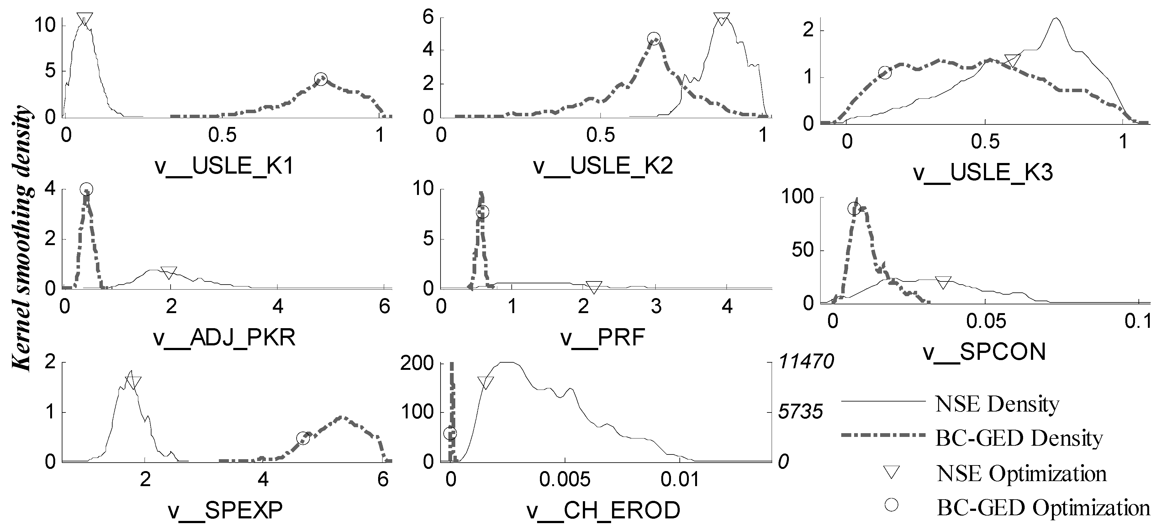
Targeted on sediment parameters, the posterior distribution and optimal value of sediment parameters estimated by the multi-objective NSE approach are shown in Figure 6. This figure demonstrates that the soil USLE erodible factor of Luvisols (USLE_K2) is greater than that of Fluvisols (USLE_K3), and greater than that of Regosols (USLE_K1), i.e., the value of USLE_K2 (Luvisols) > USLE_K3 (Fluvisols) > USLE_K1 (Regosols). The posterior distribution of USLE_K1 (Regosols) is sharper than that of USLE_K2 (Luvisols), and sharper than that of USLE_K3 (Fluvisols), i.e., the uncertainty of USLE_K1 (Regosols) < USLE_K2 (Luvisols) < USLE_K3 (Fluvisols). 95% confidence interval of the posterior distribution of SPEXP is [1.33, 2.40] that is closed to the recommended range ([1.0, 2.0]) by Neitsch et al. [33].

4.2. BC-GED Approach

The BC-GED approach first uses the simulated river discharges and sediment loads by the SWAT-WB-VSA model to estimate values of BC transformation parameter (λ) based on the minimum variance constraint (Equation (21)), and then calculates BC-GED values of flow and sediment after BC transformation (Equation (20)) based on given values of kurtosis coefficient (β), respectively. Finally it calculates the likelihood value ( l ( θ | o b s ) , Equation (22)) at each MCMC iteration for flood and sediment model residuals.
Unlike the flow series, the sequence of sediment loads is discrete, and parameters of error model can only be estimated using the flood-state data. Additionally, the number of sediment data (greater than zero) is too few. Therefore, for simplification and reduction of model uncertainty, GED kurtosis coefficient for sediment model residuals (βsed) is set to a constant value of 0.672 that is the optimal inference result of single-objective BC-GED approach. Finally values of BC-GED error model parameters follow as: λflow = 0.44, λsed = 0.35, βflow = 0.65 and βsed = 0.672.
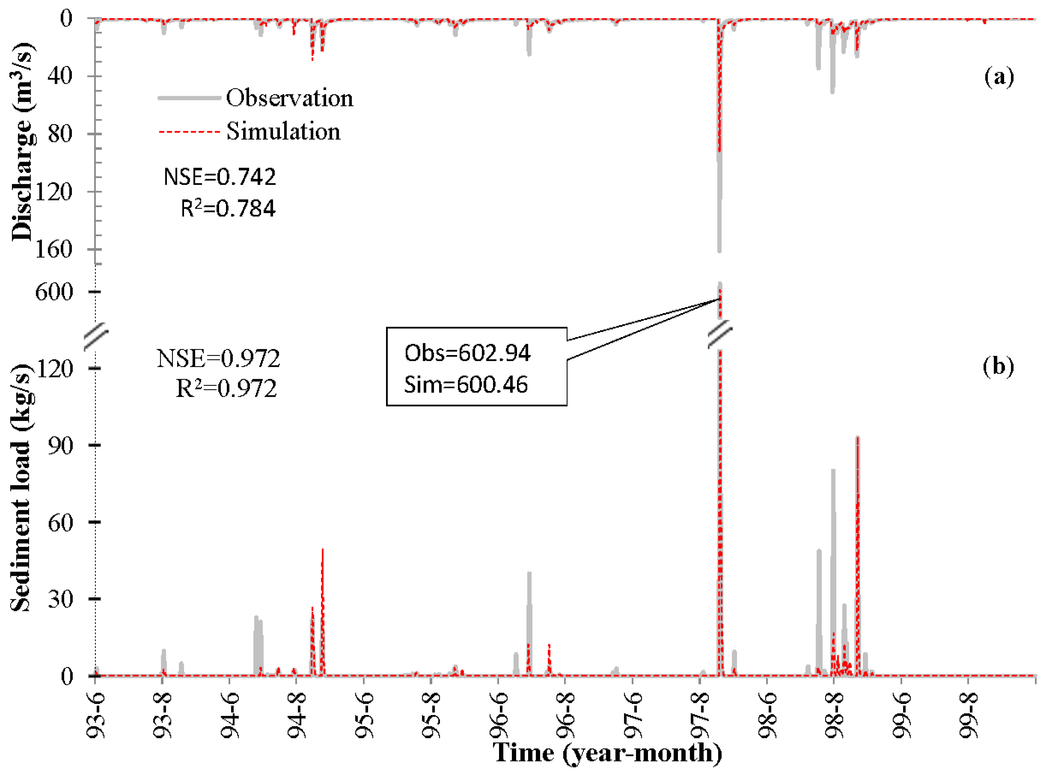
Comparison of observed and simulated river discharges and sediment loads on the daily time step during the flood season (from June to September) in the period of 1993–1999 are shown in Figure 7. The simulated data are produced by SWAT-WB-VSA with the optimal values of model parameters estimated by the multi-objective BC-GED approach. Figure 7a shows that simulated results can reproduce most of flood events, but simulated flood peaks are smaller than those of observed values in some cases, especially in extreme flood events e.g., in 1997. Figure 7b shows that SWAT-WB-VSA with the BC-GED approach also mimics the sediment loads well.
The amount of river discharges and sediment loads during the flood period in each year are shown in Table 3. In this table, the BC-GED approach markedly underestimates the river discharges of 1995~1998 and extremely underestimates sediment loads in high flow years of 1995, 1996 and 1998. And this method overestimates river discharges in the low flow years of 1994 and 1999. Nevertheless, compared with the NSE approach, it underestimates sediment loads, particularly in 1999.
Further, inspecting the error distribution assumption of BC-GED approach is shown in Figure 8, via the empirical error distribution versus the generalized error distribution (GED). In this figure, “λ”, “μ”, “σ” and “β” are the parameters of error model inferred by the BC-GED approach, where “λ” is BC transformation parameter (lambda), and “μ”, “σ” and “β” are the mean, standard deviation and kurtosis coefficient of GED function, respectively. It is noted that the flow and sediment model residuals use the different parameter set of error model.
Figure 8a shows that the inferred error distribution (GED) matches the empirical distribution of residuals well. Figure 8b shows that the inferred GED generally over-estimates the probability of positive residuals, but under-estimates that of negative residuals. Therefore, the empirical error distribution of sediment seems to be skewed. However, the error distribution of sediment is impossible to be skewed because the mean/bias of residuals is zero (“μ”; Figure 8b), and a number of residuals are zero, i.e., the mode of residuals is zero, which can guarantee the symmetry of the error distribution with zero-mean and zero-mode.
Therefore, the main reason of deviation between the empirical and the hypothetical error distribution of sediment (Figure 8b) is the statistical bias, which owes to too few samplings. In order to increase the number of statistical samplings, absolute residuals of sediment are used instead of original residuals for estimation of the empirical error distribution. The distribution of absolute residuals of sediment is inspected in Figure 8c. This figure shows the inferred GED well matches the empirical error distribution.
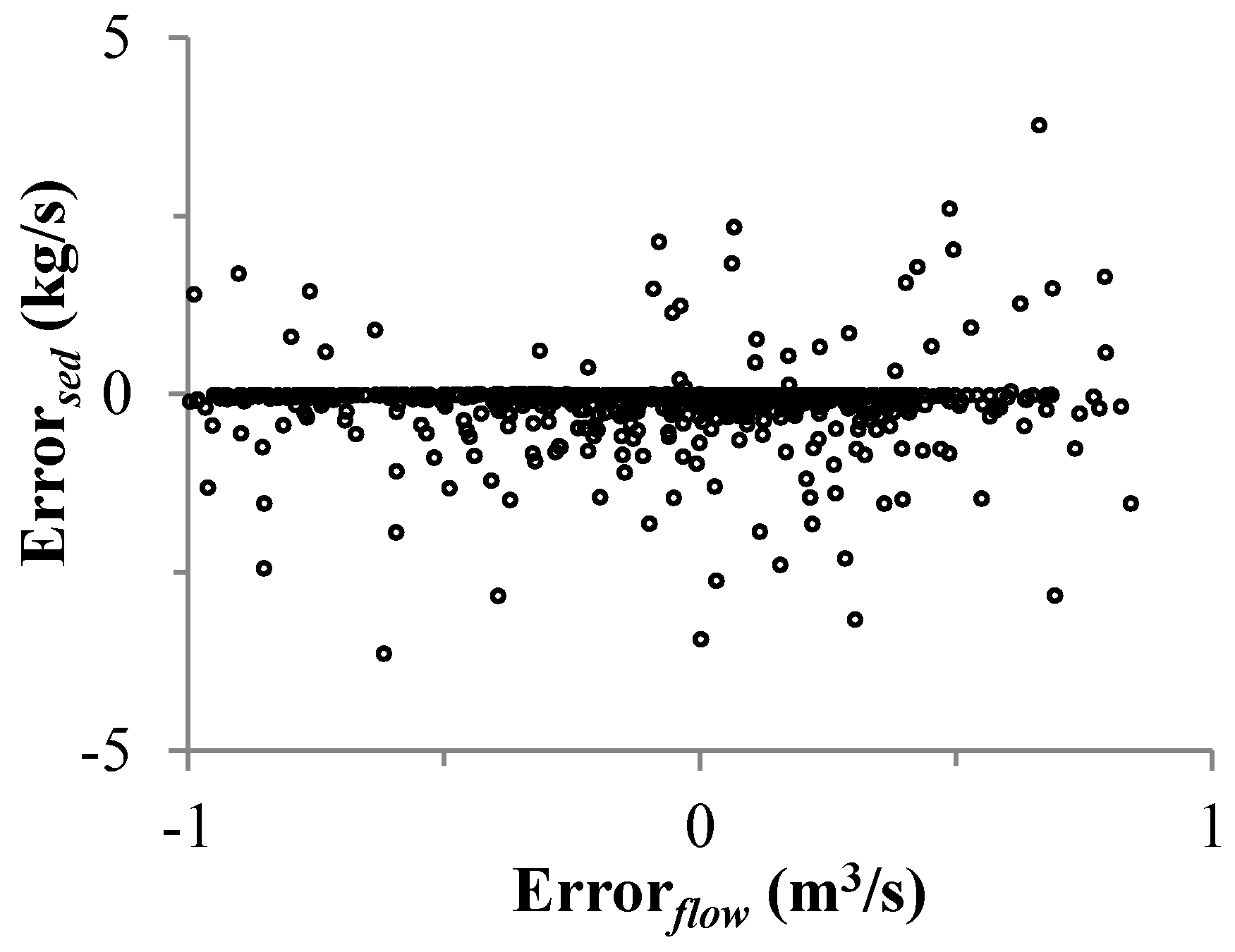
In Figure 9, we inspect the assumption of independence between the flow ( e flow ) and sediment ( e sed ) model residuals after the BC transformation. This figure shows e sed are obviously independent of e flow , which also pass the Spearman test with 5% significance level for “independence” hypothesis [36]. Therefore, the BC-GED approach belongs to a formal likelihood function of which the inferred model residuals fulfill the statistical assumption [22,23].
Computed by SWAT-WB-VSA with optimized parameters, average annual components of river flow and sediment for the BC-GED approach are shown in Table 4. This table shows that runoff components are nearly the same between the multi- and single-objective BC-GED methods, where most (about 76%) of runoff is from underground flow, and the amount of groundwater return flow is close to that of interflow, but greater than that of overland flow. However, pathways of groundwater loss are bit different. The multi-objective method concludes that some groundwater loss occurs due to evaporation. The component analysis of sediment loads in the main channel indicates that all main channels have sediment deposition problem, and nearly 18% of sediments eroded from hillslopes/HRUs deposit in the main channel, which is in agreement with results in Table 3, where the amount of simulated sediment loads is close to zero in 1999.
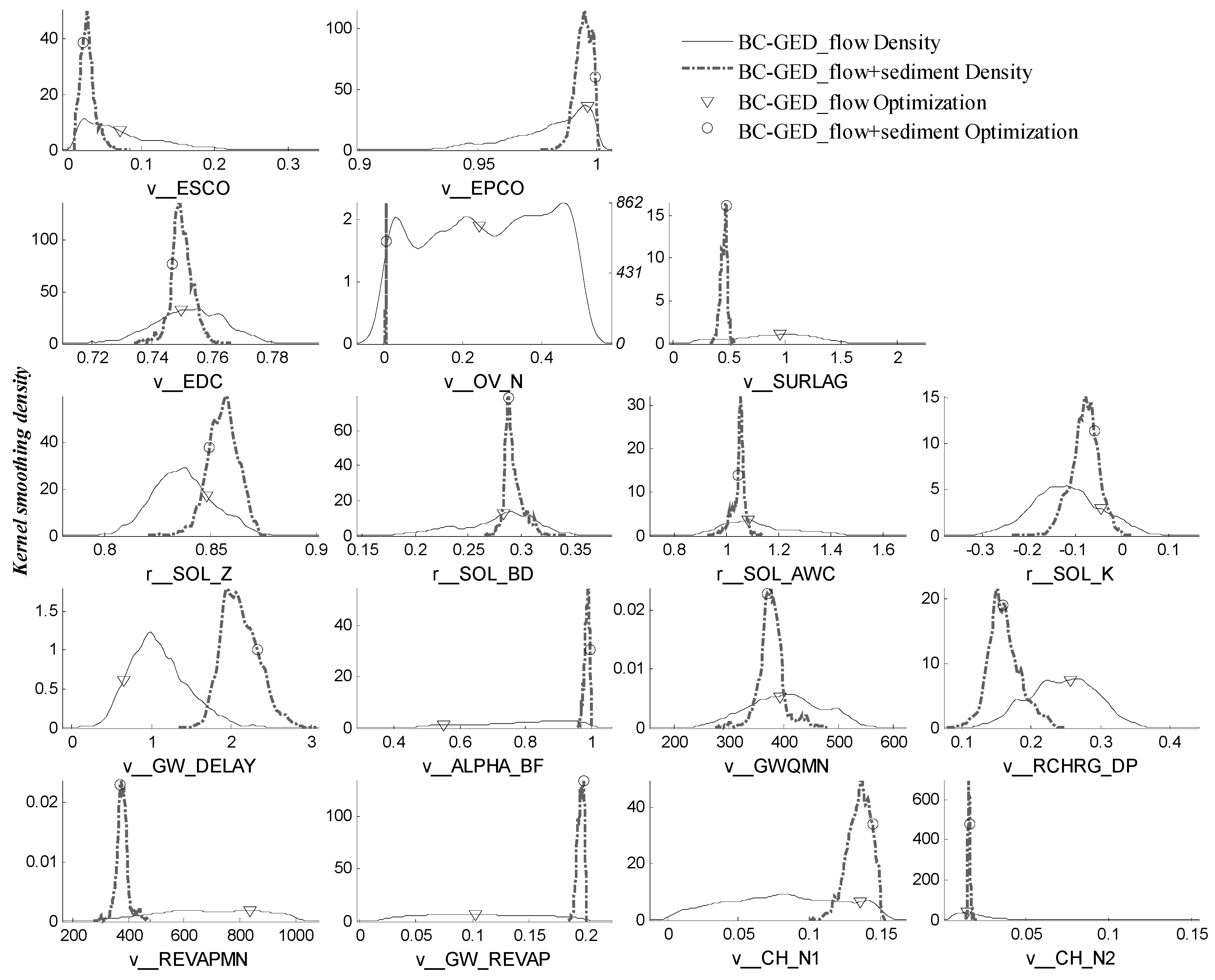
The posterior parameter distributions (after kernel smoothing) and optimal values of flow parameters estimated by the multi- and single-objective BC-GED approaches are shown in Figure 10. In this figure, the posterior distributions of flow parameters estimated by the multi-objective BC-GED approach are obviously sharper than those estimated by the single-objective method, and even some parameters (such as OV_N and CH_N2) nearly become constant values. However, optimal parameter values of the multi-objective BC-GED approach, such as the effective soil depth (EDC) and the soil property parameters (e.g., SOL_Z, SOL_BD, SOL_AWC and SOL_K), are close to those of the single-objective method, which is in agreement with the results in Table 4, where the average annual runoff components are nearly no difference between the multi- and single-objective BC-GED methods.
In Figure 10, however, optimal values of groundwater parameters are different between the multi- and single-objective BC-GED methods. For example, values of recharge partition coefficient (RCHRG_DP) in the multi-objective method are obviously less than those of single-objective method. But values of groundwater evaporation conversion coefficient (GW_REVAP) are greater, which is in agreement with results in Table 4 for the BC-GED approach. In that table, the amount of groundwater evaporation by the multi-objective method is greater than that by the single-objective method, but the amount of deep aquifer recharge is less. It may result from the inter-correlation and equifinality of different parameters that lack physical meaning, e.g., the total groundwater loss (including evaporation and deep percolation of shallow aquifer) is nearly the same between the multi- and single- response methods (Table 4).
The posterior parameter distributions and optimal values of sediment parameters estimated by the multi-objective BC-GED approach are shown in Figure 6. This figure shows that the optimal value of USLE erodible factor of Regosols (USLE_K1) is greater than that of Luvisols (USLE_K2), and greater than that of Fluvisols (USLE_K3), i.e., the value of USLE_K1 (Regosols) > USLE_K2 (Luvisols) > USLE_K3 (Fluvisols). The posterior distribution of USLE_K1 (Regosols) is sharper than that of USLE_K2 (Luvisols), and sharper than that of USLE_K3 (Fluvisols), i.e., the uncertainty of USLE_K1 (Regosols) < USLE_K2 (Luvisols) < USLE_K3 (Fluvisols). The values of channel erodible factor (CH_EROD) approach zero, which means the main channels are nearly non-erodible. It is in agreement with the result in Table 4, where the sediment deposition occurs in all main channels.

5. Discussion

5.1. Effects of Multi-Objective Approach

Comparison of the best simulation results (corresponding to the maximum value of likelihood function) between the multi- and single- object NSE/BC-GED approaches demonstrates that the average annual runoff components (Table 4) and the most optimal flow-parameters (Figure 5 and Figure 10) are similar, which means that the effect of multi-objective NSE/BC-GED approach on river discharges is small. It may result from two reasons: (1) parameter inter-correlation and equifinality occur in the SWAT model. For example, the soil erosions from HRUs depend on not only the surface runoff but also the soil erodibility factor (USLE_K). In addition, USLE_K as a characteristic parameter of soil type varies with different soil types (Table 1 and Table 2). As a consequence, it is unnecessary to tune sensitive flow parameters (related to river discharges) to improve model performance of sediment loads when calibrating the flow and sediment parameters simultaneously. (2) flow parameters related directly to the sediment transport (e.g., the manning roughness coefficients of sloping surface (OV_N; Equation (7)) and main channel (CH_N2; Equation (11)) are insensitive to river discharges in this study, although they are sensitive to sediment transport (Figure 5 and Figure 10). Therefore, changes of OV_N and CH_N2 affect runoff components and river discharges slightly (Table 4) in the Baocun watershed.
Posterior distributions of flow parameters inferred by the multi-objective NSE/BC-GED approach are all sharper than those inferred by the single-objective NSE/BC-GED approach (only with river flow objective) (Figure 5 and Figure 10), especially parameters related to surface runoff and river flow velocity, such as OV_N, SURLAG, CH_N1 and CH_N2. It demonstrates that there are clearly trade-offs between the flow and sediment objectives, and multi-objective likelihood approaches decrease the uncertainty of model parameters. It is confirmed that improving information can reduce the uncertainty of model parameters [37].
In summary, the multi-objective calibration method improves the performance of sediment simulation without significantly impairing the performance of flow simulation, and reduces the uncertainty of flow parameters, especially flow concentration parameters (such as OV_N and CH_N2).

5.2. Difference between NSE and BC-GED Error Model

With the NSE approach, SWAT-WB-VSA captures extreme flood events well (Figure 3). For example, in 1997, the simulated peak flow and sediment are 158.40 m3/s and 603.47 kg/s, respectively, which are nearly equal to the observed results that are 160.99 m3/s and 602.94 kg/s, respectively. However the relative errors of baseflow and low sediment load are high, e.g., in 1999 (Table 3). A possible reason is that the NSE approach is an informal likelihood function because model residuals produced by the NSE method violate the Gaussian error distribution assumption (Figure 4) [22], and puts greater emphasis on high values [23].
The annual erosion rate of HRUs estimated by the BC-GED approach (290.5 t/(km2∙a); Table 3) is greater than that estimated by NSE approach (207.9 t/(km2∙a); Table 3). According to the Chinese standards for soil erosion published by the China Ministry of Water Resources [38], both simulated results indicate that the Baocun watershed belongs to the mild erodible gradation that ranges from 200 to 2500 t/(km2∙a) in the category of the earth and stone zone.
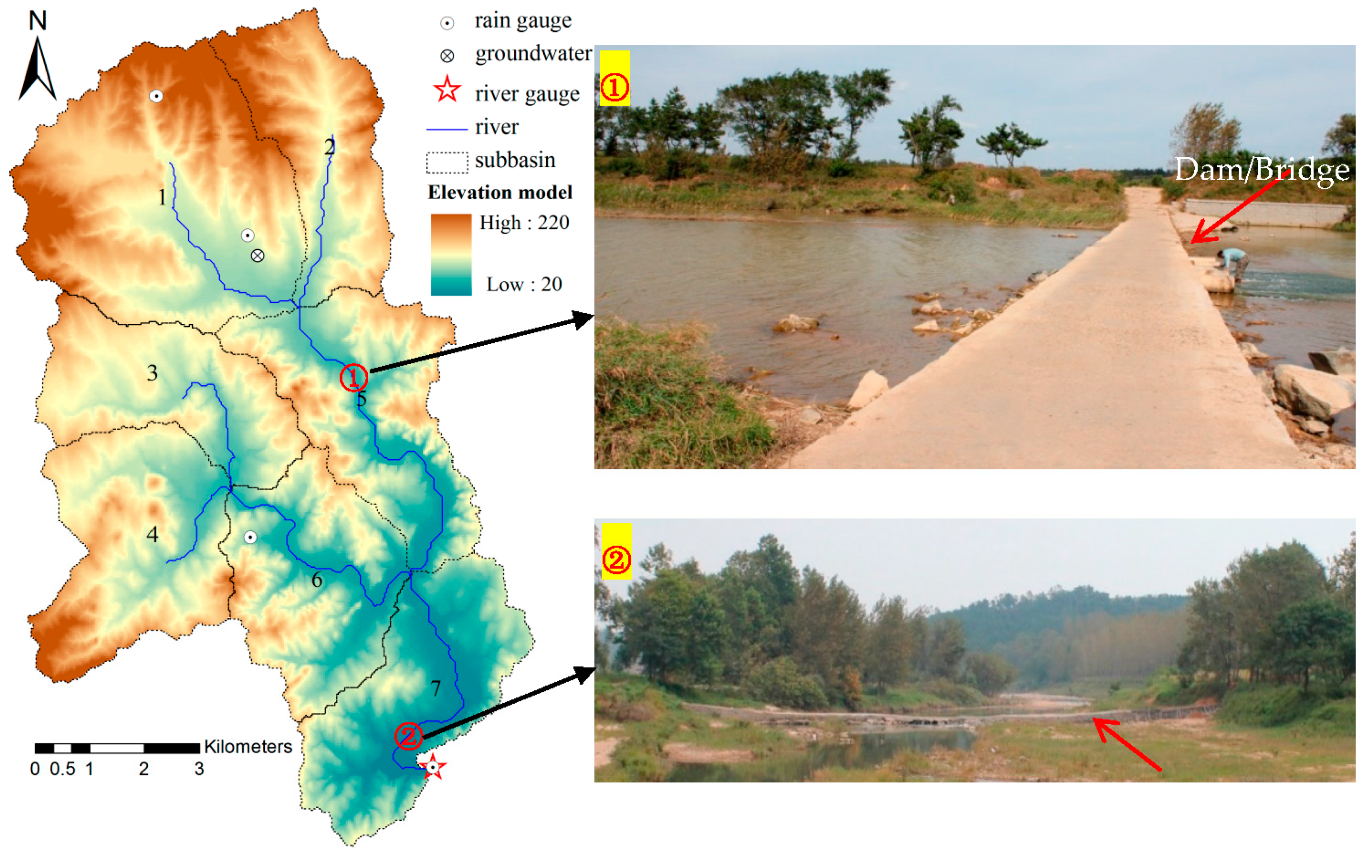
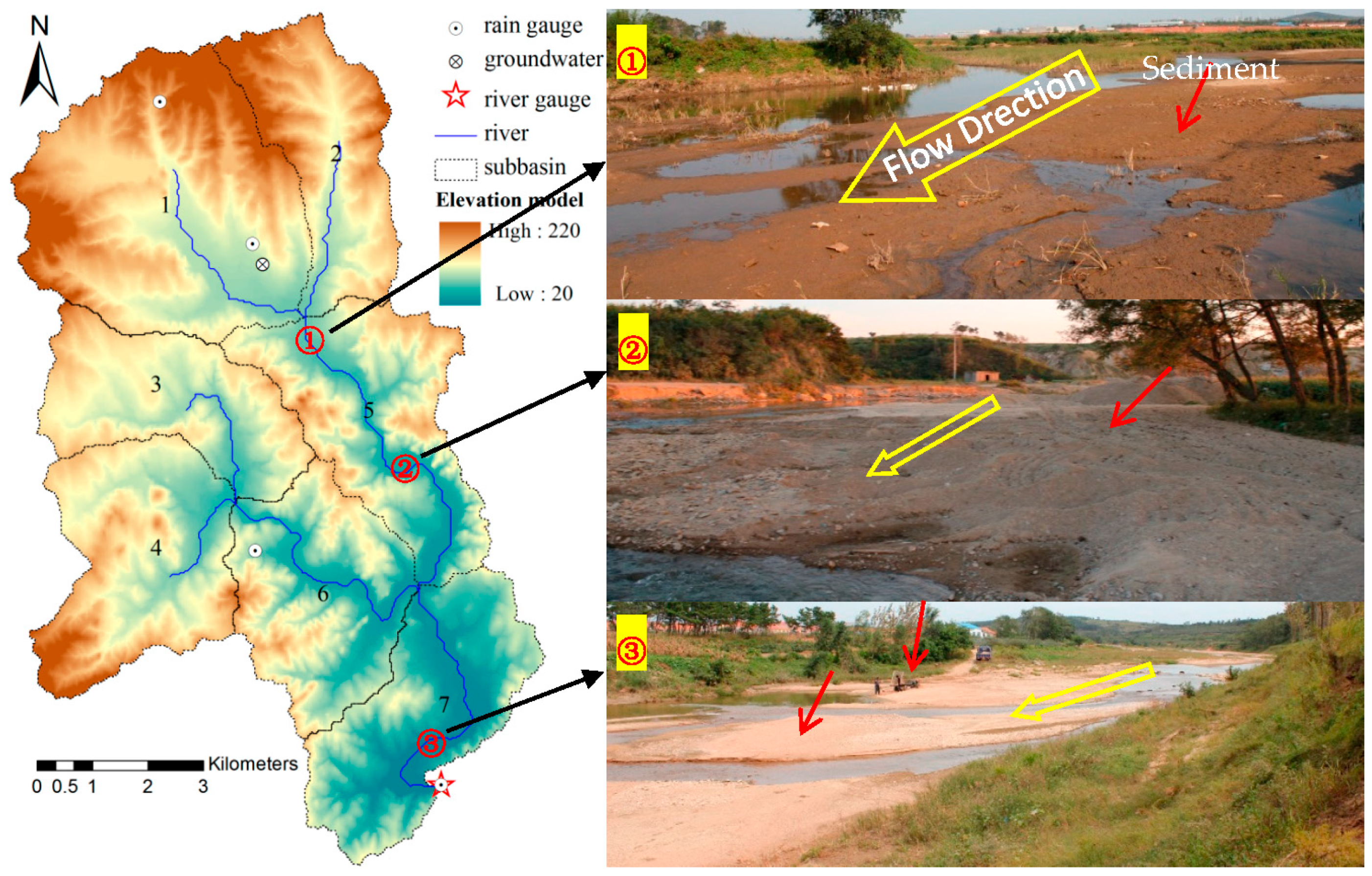
The inferred erodibility values of main channels are distinct differences between NSE and BC-GED approaches (Table 4). For the NSE approach, more than 36% of sediment loads in the watershed outlet are from erosion of main channels. By contrast, nearly 18% of sediments eroded from slopes/HRUs deposit in the main channels for the BC-GED approach. Field survey shows that local residents had built some small dams in the main channel for water supply, irrigation and transportation. Two physical photographs of run-off-the-river impoundments are shown in Figure 11. These “reservoirs” have small effect on the daily runoff because of small storage capacity, but obviously affect sediment transport because of reducing flow velocity (except for extreme floods owing to low height dam) that impacts on the sediment transport capacity of flow and results in sediment deposition. Therefore, small dams intercepted some sediments in the main channel, which is also reflected in the recorded sediment-load data that suddenly fell to zero values after the flood peak. Some photographic evidence of deposition sediments in the main channels of the Baocun watershed is shown in Figure 12. Therefore, the inferred sediment-loads by the BC-GED approach are more reasonable than that by the NSE method, possibly because the BC-GED approach is a formal likelihood function which balances consideration of the high and low outcomes (Figure 8 and Figure 9).
The difference between NSE and BC-GED approaches is also reflected in the inferred posterior distribution of channel erodibility factor (CH_EROD; Figure 6) that determines the erodibility of main channel. The CH_EROD estimated by the BC-GED approach almost equals zero, which corresponds to the non-erodible channel. By contrast, the CH_EROD estimated by the NSE approach has much larger value and wider range (i.e., higher uncertainty).
The soil USLE erodibility factors (USLE_K) inferred by the NSE approach are completely different to those determined by the BC-GED approach. Driessen et al. [39] summarized the major soils in the world and pointed out that: (1) Regosols in sloping areas is prone to erosion because of low coherence of the matrix material; (2) Luvisols usually has a stable blocky structure except for high silt content of surface soil that may be sensitive to slaking and erosion; (3) Fluvisols erosion/deposition depends on its location: usually the erosion occurs in the upper reach and the deposition occurs in the lower reach. According to the study of Driessen et al. [39], USLE_K estimated by the BC-GED approach may be more reasonable (Figure 6): value of USLE_K1 (i.e., USLE erodible factor of Regosols) is the largest, value of USLE_K2 (Luvisols) is less, and value of USLE_K3 (Fluvisols) is the least with highest uncertainty owing to the wide slope range (i.e., 9.5–24.3 TI) of fluvisols in the Baocun watershed, where the sediment erosion and deposition occur together.
The order of USLE_K empirical values for regosols, luvisols and fluvisols estimated by the Williams’ equation [3] in Table 1 also confirmed the reasonability of inferred results by the BC-GED approach. Note that the optimized USLE_K value in this study includes some effects of other factors such as topography, land use and human activity factors. Therefore, it is not surprising that the optimized USLE_K value is larger than the empirical value (Table 1).
The parameters of PRF, SPCON, and SPEXP are used to calculate the channel sediment transport capacity (Equation (10)). Figure 6 shows that values of PRF and SPCON estimated by the BC-GED approach are smaller than those estimated by the NSE approach, but the value of SPEXP is obviously larger. As a result, the channel sediment transport capacity estimated by the BC-GED approach is more sensitivity to the river discharges than that estimated by the NSE approach (Equation (10)). It may result from that SWAT-WB-VSA with the BC-GED approach underestimates some flood peaks, and there are large differences between the high- and low- values of sediment loads (Figure 3 and Figure 7).
Although Neitsch et al. [33] recommended the closed interval [1,2] as the range of SPEXP that reflects the power of flow velocity-transporting sediments, the simplified Bagnold equation (Equation (10)) is a half-theoretical and half-empirical formula, and even the study of Guo [40] showed that the power of flow velocity in Yangtze river can reach 4.5. So the value of SPEXP (power) depends on the channel morphology, and SPEXP value estimated by BC-GED approach may be also reasonable.
In summary, according to the field investigations and previous studies, the erodibility of soil and main channel inferred by the multi-objective formal likelihood (BC-GED) approach are more reasonable than that inferred by the NSE approach.

6. Conclusions

Hydrological models have become more and more complex as they are developed in consideration of not only hydrological processes but also ecological and environmental processes, such as watershed soil erosion and pollutants driven by flow. Extended model functions would lead to increase the number of model parameters and thus the uncertainty of modeling outcomes. Meanwhile additional observation information, such as sediment and pollutant load, which are highly related to watershed discharges, could be used to reduce flow model uncertainty. Therefore, it is important to study how to combine multiple observation information for calibration of complex hydrological model. This study proposed a method to convert different single objectives into a likelihood function for multi-objective calibration based on the Bayesian inference.
Our results show that the multi-objective approach (compared with the single-objective approach) improves the performance of sediment simulation without obviously impairing the performance of flow simulation, and reduce the uncertainty of flow parameters, especially flow concentration parameters.
With the NSE approach, SWAT-WB-VSA captures extreme flood events well, but fail to mimic low values of river discharge and sediment load. As a result, the NSE approach infers unreasonable results, e.g., 36% of sediment loads in the watershed outlet are from erosion of main channels. A possible reason is that the NSE approach is an informal likelihood function, and puts greater emphasis on high values. By contrast, the BC-GED approach approximates a formal likelihood function, and balances consideration of the high- and low- values. Therefore, the inferred river discharges, sediment loads and model parameter values by the BC-GED approach are more reasonable and consistent with the field survey results and previous related-studies. This method even discriminates the non-erodible characteristic of channels.
The SWAT-WB-VSA simulation results calibrated by the multi-objective BC-GED approach show that the Baocun watershed belongs to a mild erodible area where the annual erosion rate of slope is 290.5 t/(km2∙a) and nearly 18% of sediments eroded from slopes deposit in the main channels.

Author Contributions

Conceptualization, Methodology and Formal Analysis, Q.-B.C. and X.C.; Writing—Original Draft Preparation, Q.-B.C.; Software, J.W.; Writing—Review and Editing, Z.-C.Z., R.-R.Z., Y.-Y.X, C.R.-I. and A.S.

Funding

This research was funded by [the National Key Research and Development Program supported by the Ministry of Science and Technology of China] grant number [2016YFC0401501]; [the Fundamental Research Funds for the Central Universities] grant number [2018B10714, 2018B44714 and B14020167]; [the National Natural Science Foundation of China] grant number [41601013, 41571130071 and 41771025] and [the Natural Science Foundation of Jiangsu Province, China] grant number [BK20150809].

Acknowledgments

We are grateful to the Hydrology and Water Resource Survey Bureau of Weihai for providing hydrologic data, the National Meteorological Information Center, China Meteorological Administration (CMA) for providing climate data, the computing facilities of Freie Universität Berlin (ZEDAT) for computer time. We would also like to thank Cong-Rong Yu for reviewing the English language, and three anonymous reviewers for their constructive comments that led to significant improvements to the paper.

Conflicts of Interest

The authors declare no conflicts of interest.

References

  1. Gassman, P.W.; Reyes, M.R.; Green, C.H.; Arnold, J.G. The Soil and Water Assessment Tool: Historical Development, Applications, and Future Research Directions. Trans. ASABE 2007, 50, 1211–1250. [Google Scholar] [CrossRef] [Green Version]
  2. Cheng, Q.-B.; Reinhardt-Imjela, C.; Chen, X.; Schulte, A.; Ji, X.; Li, F. Improvement and comparison of the rainfall-runoff methods in SWAT at the monsoonal watershed of Baocun, Eastern China. Hydrol. Sci. J. 2016, 61, 1460–1476. [Google Scholar] [CrossRef]
  3. Williams, J.R. Chapter 25: The EPIC model. In Computer Models of Watershed Hydrology; Singh, V.P., Ed.; Water Resources Publications: Highlands Ranch, CO, USA, 1995; pp. 909–1000. [Google Scholar]
  4. Bagnold, R.A. Bed load transport by natural rivers. Water Resour. Res. 1977, 13, 303–312. [Google Scholar] [CrossRef]
  5. Williams, J.R. SPNM, a Model for Predicting Sediment, Phosphorus, and Nitrogen Yields from Agricultural Basins. J. Am. Water Resour. Assoc. 1980, 16, 843–848. [Google Scholar] [CrossRef]
  6. Gebremicael, T.G.; Mohamed, Y.A.; Betrie, G.D.; van der Zaag, P.; Teferi, E. Trend analysis of runoff and sediment fluxes in the Upper Blue Nile basin: A combined analysis of statistical tests, physically-based models and landuse maps. J. Hydrol. 2013, 482, 57–68. [Google Scholar] [CrossRef]
  7. Arnold, J.G.; Moriasi, D.N.; Gassman, P.W.; Abbaspour, K.C.; White, M.J.; Srinivasan, R.; Santhi, C.; Harmel, R.D.; Griensven, A.V.; Liew, M.W.V. SWAT: Model use, calibration, and validation. Trans. ASABE 2012, 55, 1345–1352. [Google Scholar] [CrossRef]
  8. Lu, S.; Kayastha, N.; Thodsen, H.; Van, G.A.; Andersen, H.E. Multiobjective calibration for comparing channel sediment routing models in the soil and water assessment tool. J. Environ. Qual. 2014, 43, 110–120. [Google Scholar] [CrossRef] [PubMed]
  9. Gupta, H.V.; Sorooshian, S.; Yapo, P.O. Toward improved calibration of hydrologic models: Multiple and noncommensurable measures of information. Water Resour. Res. 1998, 34, 751–763. [Google Scholar] [CrossRef] [Green Version]
  10. Efstratiadis, A.; Koutsoyiannis, D. One decade of multi-objective calibration approaches in hydrological modelling: A review. Hydrol. Sci. J. 2010, 55, 58–78. [Google Scholar] [CrossRef]
  11. Abbaspour, K.C.; Yang, J.; Maximov, I.; Siber, R.; Bogner, K.; Mieleitner, J.; Zobrist, J.; Srinivasan, R. Modelling hydrology and water quality in the pre-alpine/alpine Thur watershed using SWAT. J. Hydrol. 2007, 333, 413–430. [Google Scholar] [CrossRef]
  12. Wang, Y.; Brubaker, K. Multi-objective model auto-calibration and reduced parameterization: Exploiting gradient-based optimization tool for a hydrologic model. Environ. Model. Softw. 2015, 70, 1–15. [Google Scholar] [CrossRef]
  13. Bekele, E.G.; Nicklow, J.W. Multi-objective automatic calibration of SWAT using NSGA-II. J. Hydrol. 2007, 341, 165–176. [Google Scholar] [CrossRef]
  14. Vrugt, J.A.; Gupta, H.V.; Bastidas, L.A.; Bouten, W.; Sorooshian, S. Effective and efficient algorithm for multiobjective optimization of hydrologic models. Water Resour. Res. 2003, 39, 1214. [Google Scholar] [CrossRef]
  15. Deb, K.; Pratap, A.; Agarwal, S.; Meyarivan, T. A fast and elitist multiobjective genetic algorithm: NSGA-II. IEEE Trans. Evol. Comput. 2002, 6, 182–197. [Google Scholar] [CrossRef] [Green Version]
  16. Vrugt, J.A.; Robinson, B.A. Improved evolutionary optimization from genetically adaptive multimethod search. Proc. Natl. Acad. Sci. USA 2007, 104, 708–711. [Google Scholar] [CrossRef] [PubMed] [Green Version]
  17. Huang, Y. Multi-objective calibration of a reservoir water quality model in aggregation and non-dominated sorting approaches. J. Hydrol. 2014, 510, 280–292. [Google Scholar] [CrossRef]
  18. Reichert, P.; Schuwirth, N. Linking statistical bias description to multiobjective model calibration. Water Resour. Res. 2012, 48, 184–189. [Google Scholar] [CrossRef]
  19. Cheng, Q.B.; Chen, X.; Cheng, D.D.; Wu, Y.Y.; Xie, Y.Y. Improved Inverse Modeling by Separating Model Structural and Observational Errors. Water 2018, 10, 1151. [Google Scholar] [CrossRef]
  20. Li, B.; Liang, Z.; He, Y.; Hu, L.; Zhao, W.; Acharya, K. Comparison of parameter uncertainty analysis techniques for a TOPMODEL application. Stoch. Environ. Res. Risk Assess. 2017, 31, 1045–1059. [Google Scholar] [CrossRef]
  21. Tang, Y.; Marshall, L.; Sharma, A.; Ajami, H. A Bayesian alternative for multi-objective ecohydrological model specification. J. Hydrol. 2018, 556, 25–38. [Google Scholar] [CrossRef]
  22. Cheng, Q.; Chen, X.; Xu, C.; Reinhardt-Imjela, C.; Schulte, A. Improvement and comparison of likelihood functions for model calibration and parameter uncertainty analysis within a Markov chain Monte Carlo scheme. J. Hydrol. 2014, 519, 2202–2214. [Google Scholar] [CrossRef]
  23. Cheng, Q.; Chen, X.; Xu, C.; Zhang, Z.; Reinhardt-Imjela, C.; Schulte, A. Using maximum likelihood to derive various distance-based goodness-of-fit indicators for hydrologic modeling assessment. Stoch. Environ. Res. Risk Assess. 2018, 32, 949–966. [Google Scholar] [CrossRef]
  24. FAO/IIASA/ISRIC/ISSCAS/JRC. Harmonized World Soil Database, Version 1.1; FAO: Rome, Italy; IIASA: Laxenburg, Austria, 2009. [Google Scholar]
  25. Ministry of Water Resources of China. Code for Liquid Flow Measurement in Open Channels (GB 50179-2015); China Planning Press: Beijing, China, 2016. (In Chinese)
  26. Ministry of Water Resources of China. Code for Measurement of Suspended Load in Open Channels (GB/T 50159-2015); China Planning Press: Beijing, China, 2016. (In Chinese)
  27. White, E.D.; Easton, Z.M.; Fuka, D.R.; Collick, A.S.; Adgo, E.; McCartney, M.; Awulachew, S.B.; Selassie, Y.G.; Steenhuis, T.S. Development and application of a physically based landscape water balance in the SWAT model. Hydrol. Process. 2011, 25, 915–925. [Google Scholar] [CrossRef]
  28. Yustres, Á.; Asensio, L.; Alonso, J.; Navarro, V. A review of Markov Chain Monte Carlo and information theory tools for inverse problems in subsurface flow. Comput. Geosci. 2012, 16, 1–20. [Google Scholar] [CrossRef]
  29. Marshall, L.; Nott, D.; Sharma, A. Hydrological model selection: A Bayesian alternative. Water Resour. Res. 2005, 41, W10422. [Google Scholar] [CrossRef]
  30. Vrugt, J.A.; Braak, C.J.F.T.; Diks, C.G.H.; Robinson, B.A.; Hyman, J.M.; Higdon, D. Accelerating Markov Chain Monte Carlo Simulation by Differential Evolution with Self-Adaptive Randomized Subspace Sampling. Int. J. Nonlinear Sci. Numer. Simul. 2009, 10, 273–290. [Google Scholar] [CrossRef] [Green Version]
  31. Douglas-Mankin, K.R.; Srinivasan, R.; Arnold, J.G. Soil and Water Assessment Tool (SWAT) Model: Current Developments and Applications. Trans. ASABE 2010, 53, 1423–1431. [Google Scholar] [CrossRef]
  32. Kumarasamy, K.; Belmont, P. Calibration Parameter Selection and Watershed Hydrology Model Evaluation in Time and Frequency Domains. Water 2018, 10, 710. [Google Scholar] [CrossRef]
  33. Neitsch, S.L.; Arnold, J.G.; Kiniry, J.R.; Williams, J.R. Soil and Water Assessment Tool Theoretical Documentation Version 2009; Texas Water Resources Institute Technical Report No. 406; Texas A&M University System: College Station, TX, USA, 2011. [Google Scholar]
  34. Nash, J.E. River flow forecasting through conceptual models, I: A discussion of principles. J. Hydrol. 1970, 10, 398–409. [Google Scholar] [CrossRef]
  35. Strahler, A.N. Quantitative analysis of watershed geomorphology. Eos Trans. Am. Geophys. Union 1957, 38, 913–920. [Google Scholar] [CrossRef]
  36. Hollander, M.; Wolfe, D.A. Nonparametric Statistical Methods; Wiley: New York, NY, USA, 1973. [Google Scholar]
  37. Goodman, D. Extrapolation in Risk Assessment: Improving the Quantification of Uncertainty, and Improving Information to Reduce the Uncertainty. Hum. Ecol. Risk Assess. Int. J. 2002, 8, 177–192. [Google Scholar] [CrossRef]
  38. Ministry of Water Resources of the People’s Republic of China. Standards of Classification and Gradation of Soil Erosion (SL 190-2007); Water Power Press: Beijing, China, 2008. (In Chinese)
  39. Driessen, P.; Deckers, J.; Spaargaren, O.; Nachtergaele, F. Lecture Notes on the Major Soils of the World. Report of the World Soil Resources; Food and Agriculture Organization: Rome, Italy, 2001. [Google Scholar]
  40. Guo, J. Logarithmic matching and its applications in computational hydraulics and sediment transport. J. Hydraul. Res. 2002, 40, 555–565. [Google Scholar] [CrossRef]
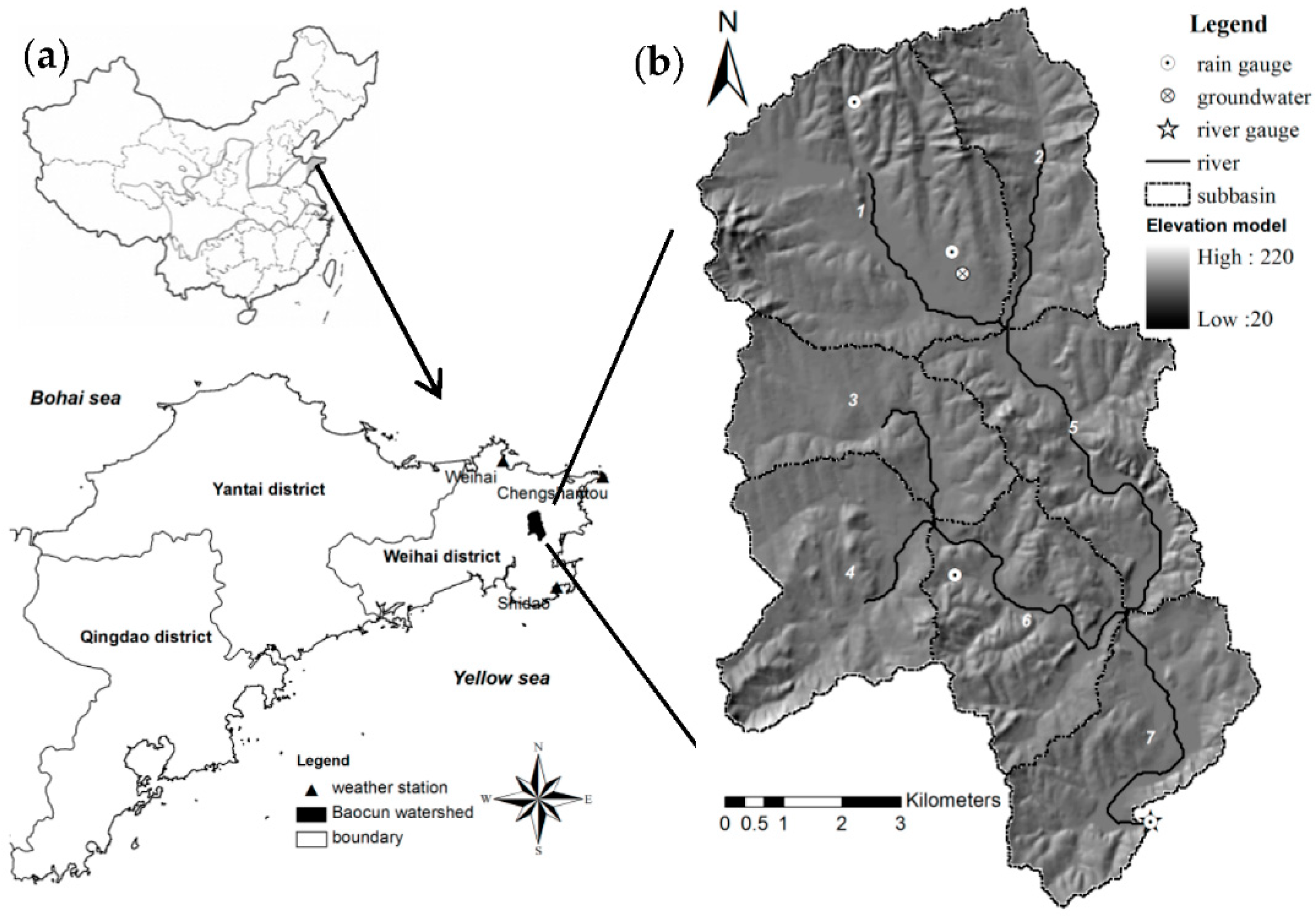
Figure 1. Location and topography of the Jiaodong peninsula (a) and the Baocun watershed (b) as well as the position of gauging stations.
Water 10 01662 g001
Figure 2. The spatial data in the Baocun watershed for the SWAT-WB-VSA model: (a) Topographic index ln(A/tanβ); (b) soil type map; and (c) average annual land use map.
Water 10 01662 g002
Figure 3. Optimal simulation results of the NSE approach during the flood season (from June to September) in 1993–1999: (a) comparison of the observed and simulated river discharges; and (b) comparison of the observed (black solid line) and simulated (red dot line) sediment loads.
Water 10 01662 g003
Figure 4. Empirical probability density of model residuals (black line) versus the assumed Gaussian distribution (red dash line) of the NSE approach: (a) flow; and (b) sediment.
Water 10 01662 g004
Figure 5. Comparison of the posterior distribution and optimal value (point) of flow parameters estimated by the multi- (dash line) and single-objective (solid line) NSE approaches.
Water 10 01662 g005
Figure 6. Comparison of the posterior distribution and optimal value (point) of sediment parameters estimated by the multi-objective NSE and BC-GED approaches.
Water 10 01662 g006
Figure 7. Optimal simulation results of BC-GED approach during the flood season (from June to September) in 1993–1999: (a) comparison of the observed and simulated river discharges; and (b) comparison of the observed (black solid line) and simulated (red dot line) sediment loads.
Water 10 01662 g007
Figure 8. Empirical probability density (black circle) of model residuals versus the inferred GED (red dash line): (a) Flow; (b) Sediment; and (c) Absolute residuals of sediment.
Water 10 01662 g008
Figure 9. Diagnosis of the independence between flow and sediment model residuals after the BC transformation for the BC-GED approach.
Water 10 01662 g009
Figure 10. Comparison of the posterior distribution and optimal value (point) of flow parameters estimated by the single- (solid line) and multi-objective (dash line) BC-GED approaches.
Water 10 01662 g010
Figure 11. Two physical photographs of small dams across the main channel in the Baocun watershed.
Water 10 01662 g011
Figure 12. Photographic evidences of deposition sediments in the main channels.
Water 10 01662 g012
Table 1. The physical characteristics of three major soil types in the Baocun watershed.
Soil TypesSoil Particle Distribution (%) aOrganic Carbon (% Weight)Conductivity (10−6 m/s)USLE_K b
GravelSandSiltClay
Regosols203827150.9870.174
Luvisols43936210.7460.173
Fluvisols9721450.41330.143
a Gravel: >2 mm; Sand: 2–0.05 mm; Silt: 0.05–0.002 mm; Clay: <0.002 mm; b Units: 0.013 ton m2 h/(m3 ton cm).
Table 2. Description of model parameters and their ranges.
CategoriesParameterRangeAlter Type aDefinition
MinMax
EvapotranspirationESCO0.011v__Soil evaporation compensation factor
EPCO0.011v__Plant uptake compensation factor
Surface waterEDC01v__Effective depth of the soil profile
OV_N0.0050.5v__Manning’s “n” value for overland flow
SURLAG024v__Surface runoff lag coefficient
Soil waterSOL_Z10%3r__Soil thickness
SOL_BD40%2r__Moist bulk density
SOL_AWC1%4r__Available water capacity of the soil layer
SOL_K1%11r__Saturated hydraulic conductivity
Ground waterGW_DELAY060v__Groundwater delay time (days)
ALPHA_BF01v__Baseflow recession constant
GWQMN01000v__Threshold depth of water in the shallow aquifer required for return flow to occur (mm)
RCHRG_DP01v__Deep aquifer percolation fraction
REVAPMN01000v__Threshold depth of water in the shallow aquifer for revaporization (mm)
GW_REVAP0.020.2v__Groundwater revaporization coefficient
Tributary/main channelCH_N10.0050.15v__Manning’s “n” value for the tributary channels
CH_N20.0050.15v__Manning’s “n” value for the main channels
MUSLEUSLE_K101v__Regosols erodibility factor (Uphill)
USLE_K201v__Luvisols erodibility factor (Sidehill)
USLE_K301v__Fluvisols erodibility factor (Foothill)
ADJ_PKR010v__Subbasin peak rate adjustment factor
Sediment transportPRF010v__Main channel peak rate adjustment factor
SPCON0.00010.1v__Linear coefficient in sediment transport
SPEXP0.00016v__Exponent coefficient in sediment transport
CH_EROD01v__Channel erodibility factor
a Alter type is a scheme to change parameter values during model calibration, where “v__” indicates that the active value replaces the initial value; “r__” means a relative change to the initial value, i.e., the active value adds one and then multiplies the initial value.
Table 3. Comparison of total flow and sediment amount between simulation and observation during flood season for each year.
CategoriesMethods1993199419951996199719981999Total
Flow (×86,400 m3)Observation105.7201.2133.6142.2258.8376.70.21218.4
Simulation (NSE)23.5203.7127.7147.3275.4292.110.21079.9
Simulation (BC-GED)91.9213.5117.0135.9198.6255.620.81033.4
Sediment (Ton)Observation1634.38988.71081.45205.854,928.725,444.90.097,283.8
Simulation (NSE)251.810,138.03659.94784.657,388.220,788.1302.497,313.0
Simulation (BC-GED)513.29312.0718.12606.356,632.315,452.12.485,236.4
Table 4. The average annual component of simulated flow and sediment.
CategoriesNSE ApproachBC-GED Approach
FlowFlow + SedFlowFlow + Sed
Flow (mm)Evaporation489.50492.90520.60521.20
Surface flow37.0437.1065.0963.17
Lateral flow12.4913.1790.8290.39
Ground flow199.84197.43102.47107.18
Revaporization76.7374.310.0012.94
Deep percolation3.343.5538.8225.73
Sediment a (Ton)Total slope erosion 18,101.2 25,185.9
Total river erosion 10,246.1 −4445.9
Level_2 river_5 erosion 2863.1 −1567.7
Level_2 river_6 erosion 1925.5 −1276.1
Level_3 river_7 erosion 5457.5 −1602.0
a Positive value: erosion; negative value: deposition.