Performance Assessment of Event-Based Ensemble Landslide Susceptibility Models in Shihmen Watershed, Taiwan

Abstract

While multi-year and event-based landslide inventories are both commonly used in landslide susceptibility analysis, most areas lack multi-year landslide inventories, and the analysis results obtained from the use of event-based landslide inventories are very sensitive to the choice of event. Based on 24 event-based landslide inventories for the Shihmen watershed from 1996 to 2015, this study established five event-based single landslide susceptibility models employing logistic regression, random forest, support vector machine, kernel logistic regression, and gradient boosting decision tree methods. The ensemble methods, involving calculating the mean of the susceptibility indexes (PM), median of the susceptibility indexes (PME), weighted mean of the susceptibility indexes (PMW), and committee average of binary susceptibility values (CA) of the five single models were then used to establish four event-based ensemble landslide susceptibility models. After establishing nine landslide susceptibility models, using each inventory from the 24 event-based landslide inventories or a multi-year landslide inventory, we identified the differences in landslide susceptibility maps attributable to the different landslide inventories and modeling methods, and used the area under the receiver operating characteristic curve to assess the accuracy of the models. The results indicated that an ensemble model based on a multi-year inventory can obtain excellent predictive accuracy. The predictive accuracy of multi-year landslide susceptibility models is found to be superior to that of event-based models. In addition, the higher predictive accuracy of ensemble landslide susceptibility models than that of single models implied that these ensemble methods were robust for enhancing the model’s predictive performance in the study area. When employing event-based landslide inventories in modeling, PM ensemble models offer the best predictive ability, according to the Kruskal–Wallis test results. Areas with a high mean susceptibility index and low standard deviation, identified using the 24 PM ensemble models based on different event-based landslide inventories, constitute places where landslide mitigation measures should be prioritized.

1. Introduction

Under the impact of climate change, extreme rainfall events have caused frequent landslides and debris flows in Taiwan’s mountainous areas. In order to effectively reduce the losses caused by the landslides and debris flows, it is necessary to employ landslide susceptibility analysis to delineate those areas in watersheds that are susceptible to landslides and use this information as a reference for overall watershed management plans. The chief methods for landslide susceptibility analysis consist of heuristic, statistical, probability, and deterministic methods [1]. Many types of machine learning methods have been broadly applied to landslide susceptibility analysis in recent years and have yielded excellent results; machine learning algorithms can be classified as either parametric or nonparametric [2].

Parametric machine learning algorithms first select a form of the function and then learn the function’s coefficients through a training process. The advantage of these algorithms is that the methodology is easy to explain and understand, and the training process is short and does not require the collection of vast amounts of data; their limitation is that the prior selection of a function often constrains the learning process, the method is only suitable for simple problems, and the fit is often relatively poor. Parametric machine learning algorithms may employ logistic regression and linear discriminant analysis, and logistic regression, in particular, is often applied in landslide susceptibility analysis [3,4,5,6,7]. For their part, nonparametric machine learning algorithms do not require prior selection of the functional form and may fit the function of any form through the training process. The advantage of this approach is its versatility and ability to generate good performance for training sample data; its limitation is its need for vast amounts of data, a slow training process, and a higher chance of overfitting occurring [2]. When the training sample is too small, the nonparametric algorithm inevitably leads to inadequate training, which will reduce the accuracy [8]. The nonparametric machine learning algorithms most commonly used in landslide susceptibility analysis include the support vector machine [9,10,11,12,13,14,15], random forest [8,9,12,15,16,17,18], kernel logistic regression [10,11,19], and boosted regression tree [15,16,17].

When performing landslide susceptibility analysis, landslide inventories can be classified as either multi-year or event-based, depending on the length of data collection time in the inventory. Apart from establishing a landslide susceptibility model based on a multi-year landslide inventory [20,21,22], when the research area lacks a multi-year landslide inventory, an event-based landslide inventory and triggering factors can be used to perform susceptibility analysis [3]. When establishing an event-based landslide susceptibility model, a landslide inventory for the event and data concerning the spatial distribution of triggering factors must be available; triggering factors, such as rainfall or earthquake intensity, are taken as independent variables in the model [6,23,24,25].

When establishing a landslide susceptibility model, the input sample data set is usually divided into a training set and a testing set. After using the training set to establish a model, the testing set is used to assess the performance of the model. The sample data set commonly contains a 50:50 ratio of landslide and no-landslide samples [9,13,26,27], and the ratio of the training set sample to the testing set sample is typically 70:30 [8,12,13,26,28,29]. Furthermore, when establishing a nonparametric machine learning model, the training set is also used to perform hyperparameter optimization. During the optimization process, fivefold cross-validation [9] and tenfold cross-validation [12,30] are often used to tune the hyperparameters.

Because each modeling method has its own advantages and limitations, different models can be used to perform landslide susceptibility analysis for the same research area, but uncertainty associated with the results of these models may exist. The ensemble method can then be used to aggregate the results of different models and can delineate areas with high susceptibility and low uncertainty [16,31]. The five most commonly used ensemble methods [32] involve the calculation of mean of landslide probabilities (PM), confidence interval for the mean of landslide probabilities (CI), median of landslide probabilities (PME), weighted mean of landslide probabilities (PMW), and committee averaging (CA), respectively. The stacking ensemble method, which uses a meta-learning algorithm to combine different single models [33], was also employed to establish ensemble modes [34,35]. In this study, the landslide susceptibility models were constructed by adopting the ensemble methods, such as PM, PME, PMW, and CA.

In order to assess the performance of different event-based ensemble landslide susceptibility models, this study used event-based and multi-year landslide inventories for the Shihmen watershed to establish single and ensemble landslide susceptibility models. To assess the robustness of the ensemble methods, we used numerous landslide inventories, rather than a single one, and compared the predictive accuracy of these single models and ensemble modes, established using the same inventory. Additionally, the rainfall-triggering factors were incorporated as independent variables into the landslide susceptibility models, which contributes to the development and improvement of landslide early-warning systems. Apart from comparing the landslide susceptibilities in the different models, this study also located those areas with high landslide susceptibility within the research area, which can provide a reference for decision-making when planning landslide mitigation measures.

2. Methods

This study first employed a logistic regression model and 4 nonparametric machine learning models to establish single landslide susceptibility models; then, it used 4 ensemble methods to establish ensemble landslide susceptibility models. In addition to establishing an event-based landslide susceptibility model, based on an event-based landslide inventory, we also combined 24 event-based landslide inventories, i.e., a multi-year landslide inventory, to establish a multi-year landslide susceptibility model. We then use the receiver operating characteristics (ROC) curve, Spearman’s rank correlation coefficient, the Mann–Whitney test, and the Kruskal–Wallis test to assess the performance of different models.

2.1. Single Landslide Susceptibility Model

2.1.1. Logistic Regression (LR) Model

Because the goal of landslide susceptibility analysis is to predict whether landslides will occur in individual slope units, the dependent variables in this model consisted of the binary response variables of “landslide” and “no-landslide”, and the logistic regression developed by Menard [36] was used to establish a parametric machine learning model, which took the form shown in Equation (1):

$$\ln \left(\frac{p_i}{1-p_i}\right)={\alpha }_i+\sum _{j=1}^k{\beta }_{ij}{x}_{ij.}$$

(1)

Here, $p_i$ is the probability of landslide occurrence, ${\alpha }_i, {\beta }_{ij}$ are the coefficients, $x_{ij}$ is the value of the susceptibility factor, $i$ represents different events, and $j$ represents different susceptibility factors.

2.1.2. Random Forest (RF) Model

The random forest model proposed by Breiman [37] is a decision tree-based ensemble method and establishes multiple decision trees via the random selection of variable subsets. Because random forest models do not require any prior assumptions concerning the relationship between the independent variables and the target variable, this type of model is suitable for the analysis of large datasets with nonlinear correlations [38]. In the process of establishing different decision trees, the re-sampling of the data and the random selection of variable subsets increase the diversity of the decision trees [39]. According to Chang et al. [12], there are three reasons for random forest models’ high performance: (1) it is a form of nonparametric nature-based analysis; (2) it can determine the importance of the variables used; and (3) it can provide an algorithm for estimating missing values. This method has been extensively used in landslide susceptibility analysis in recent years, and has yielded excellent results [8,9,12,16].

2.1.3. Support Vector Machine (SVM) and Kernel Logistic Regression (KLR) Models

Support vector machines, as proposed by Vapnik [40], constitute a supervised classification method. Their special property is their ability to simultaneously maximize the geometric margin and minimize the empirical classification error, which is why they are also referred to as maximum margin classifiers [41]. SVMs perform classification by finding the hyperplane with the largest margin between two types of training data in a higher dimensional space. A non-linear kernel function can be used to map the input data onto a higher dimensional space, where a hyperplane classifying the data can be established. Kernel logistic regression is a kernelized version of linear logistic regression [42]. This method uses a kernel function to project the input data onto a higher dimensional feature space, with the goal of finding a discriminant function of distinguishing the two categories of landslide and no-landslide.

In the two previous models, the most commonly utilized kernel functions consist of linear kernel functions, polynomial kernel functions, radial basis kernel functions (RBF), and sigmoid kernel functions. Of these types, radial basis kernel functions are the most widely used [11] and offer the best predictive ability in most situations, especially in the case of nonlinear data [14]. Radial basis kernel functions are also a very popular choice for the establishment of landslide susceptibility models [43].

2.1.4. Gradient-Boosting Decision Tree (GBDT) Model

The gradient-boosting decision tree (GBDT) model proposed by Friedman et al. [44] is similar to the gradient-boost regression tree (GBRT) and multiple additive regression tree (MART) algorithms. GBDT models combine boosting and regression trees in a single algorithm [41]. Boosting relies on the minimization of the loss function at each tree spilt to improve the decision trees [45] and represents one of the learning methods offering the greatest improvement of model accuracy [17]. Rather than being fitted without any relationship with adjacent trees, GBDT trees are fitted on top of the previous trees.

2.2. Ensemble Landslide Susceptibility Model

Referring to Thuiller et al. [32], this study selected PM, PME, PMW, and CA as the ensemble methods used to aggregate the results of the 5 single models, as shown in Table 1. Among these methods, the PM ensemble model calculates the mean of the susceptibility indexes of the single models; the PME ensemble model calculates the median of the susceptibility indexes of the single models; and the PMW ensemble model calculates the weighted mean of the susceptibility indexes of the single models. To set weights, this study assigned weights to each single model, based on the accuracy calibrated by the training-event data. Additionally, the CA ensemble model first identifies the threshold value of each single model, converts the landslide susceptibility index to a binary value (landslide or no-landslide), and calculates the committee average of binary values of the 5 single models.

Table 1. The ensemble methods to aggregate the results of the selected models.

Ensemble Methods	Description
PM	Mean of susceptibility indexes. The PM ensemble model calculates the mean of the susceptibility indexes for the selected models.
PME	Median of susceptibility indexes. The PME ensemble model calculates the median of the susceptibility indexes for the selected models.
PMW	Weighted mean of susceptibility indexes. The PMW ensemble model calculates the relative importance of the weights based on the accuracies of the selected models, and then calculates the weighted mean of the susceptibility indexes for the models.
CA	Committee averaging. After identifying the threshold value of each selected model and converting the susceptibility index to binary value, the CA ensemble model calculates the average of binary values for the selected models.

2.3. Single Model Establishment Process

2.3.1. Logistic Regression (LR) Model

All slope units with landslides in each landslide inventory are included in the landslide sample, and the no-landslide samples with the same sample number as the landslide sample are also selected. A 10-fold cross-validation is then used to perform model validation. The cross-validation process is repeated 5 times to reduce the error from the split subsets, which yields the mean test accuracy for the models, established from that sample dataset. The foregoing sampling process is repeated 10 times in order to reduce sampling error, and the model with the best mean test accuracy is selected for use in subsequent analysis.

2.3.2. Nonparametric Models (RF, SVM, KLR, GBDT)

Among nonparametric machine learning algorithms, hyperparameters must be set manually before training. For example, two hyperparameters must be set in the RF model used in this study: the number of trees to fit (numtree) and the number of variables for each tree (mtry). In an SVM or KLR model employing an RBF kernel function, two hyperparameters must be set: a penalty parameter (C) and an RBF parameter (γ). In a GBDT model, three hyperparameters must be set: numtree, mtry, and learning rate. The grid search method used to tune the hyperparameters in this study is a conventional optimization method, using our preset hyperparameter subset to perform a comprehensive search. The nonparametric models used in this study and the range of their hyperparameters are shown in Table 2.

Table 2. Hyperparameter types and the range of nonparametric models.

Model	Hyperparameter	Range
RF	number of trees (numtree)	100–1500
	number of variables (mtry)	3–14
SVM	penalty parameter (C)	0.001–1000
	RBF parameter (γ)	0.001–1000
KLR	penalty parameter (C)	0.001–1000
	RBF parameter (γ)	0.001–1000
GBDT	number of trees (numtree)	100–1000
	number of variables (mtry)	5–14
	learning rate	0.1–1

The modeling process involved the selection of all slope units with landslides in each landslide inventory, to serve as the landslide sample, and the selection of a no-landslide sample with the same sample number. All the sample data were then split into a training set and testing set in a 70:30 ratio. The model training process began with hyperparameter tuning, which involved the use of the training set data and 10-fold cross-validation to perform an analysis of each hyperparameter subset, which yielded the mean training accuracy of each hyperparameter subset. The next step consisted of establishing a model using the tuned hyperparameter subset and training set data, and the testing set data were then used to perform model validation, which yielded the test accuracy. The sampling process was repeated 10 times, which yielded 10 tuned hyperparameter subsets and their corresponding models, and the model with the best test accuracy was selected for use in the subsequent analysis.

2.4. Model Performance Assessment

2.4.1. Receiver Operating Characteristic (ROC) Curve

The receiver operating characteristic (ROC) curve [46] method employs the use of threshold values to classify prediction results into 4 types: true positive (TP), false positive (FP), true negative (TN), and false negative (FN). After calculating the true positive rate (TPR) and false positive rate (FPR) for each threshold value, the resulting data points are connected up to plot an ROC curve, where the area under the curve (AUROC) represents the model’s performance and predictive accuracy. The closer the AUROC value is to 1, the better the performance of the model.

2.4.2. Inferential Statistics

This study used the Mann–Whitney test and Kruskal–Wallis test to analyze the effect of different model methods and landslide inventories on the predictive ability of the established models.

The Mann–Whitney test, which is also known as the Wilcoxon rank sum test [47,48], is a nonparametric test used to determine whether there is a difference in the dependent variables between two independent populations. The test statistic, U, is calculated using Equation (2):

$$\mathrm{U}=N_1{N}_2+\frac{N_1\left(N_1+1\right)}{2}-\sum R_1.$$

(2)

Here, N₁ and N₂ are the sample sizes in sample 1 and sample 2, where the sample with the greatest rank sum is taken as the first sample and has a rank sum of $\sum R_1$.

The Kruskal–Wallis test was first proposed by Kruskal and Wallis [49], and is a nonparametric test that extends the two-sample Wilcoxon test in the situation where there are more than two groups. The Kruskal–Wallis test does not assume a normal distribution of the underlying data. It ranks the data from smallest to largest, and assigns a rank to the data that is used to calculate the test statistic H, as shown in Equation (3). This test is used to determine whether there is a difference between the medians of K independent populations.

$$\mathrm{H}=\frac{12}{n\left(n+1\right)}\sum _{i=1}^k\frac{R_i{}^2}{n_i}-3\left(n+1\right)$$

(3)

Here, $n=n_1+n_2+\dots +n_k,n_i$ is the sample size of each sample, and $R_i$ is the rank sum of each sample.

2.4.3. Spearman’s Rank Correlation Coefficient

Spearman’s rank correlation coefficient, as proposed by Spearman [50], is a nonparametric measure used to assess the strength and direction of the association between two ranked variables, X and Y. Depending on the values of variables X and Y, this measure ranks the data and establishes paired ranks, then calculates the difference in rank for each pair, as shown in Equation (4); the value of this coefficient is between −1 and 1 [51]:

$$\mathsf{\rho }=1-\frac{6\sum d_i^2}{n\left(n^2-1\right)}$$

(4)

where $d_i$ is the difference in rank between the susceptibility index of slope units in the two models, $\mathsf{\rho }$ is the Spearman’s rank correlation coefficient, and $n$ is the sample size.

The model performance assessment methods employed in this study are summarized in Table 3.

Table 3. Description and explanation of the model performance assessment methods.

Assessment Methods	Description	Explanation
Receiver operating characteristic (ROC) curve	The area under the ROC curve (AUROC) represented the model’s performance and predictive accuracy.	AUROC ranges in value from 0 to 1. An excellent model has an AUROC near 1, and a poor performance model has an AUROC near 0.
Mann–Whitney test	The test was used to compare the predictive accuracy of multi-year model to that of event-based models.	A p-value < 0.05 indicates that the null hypothesis is rejected and a statistically significant difference between the predictive accuracy of multi-year model and that of event-based models exists.
Kruskal–Wallis test	The test was used to compare the predictive accuracy of different modeling methods.	A p-value < 0.05 indicates that null hypothesis is rejected and a statistically significant difference of the predictive accuracy of 9 modeling methods exists.
Spearman’s rank correlation coefficient	The coefficient was used for a quantitative comparison on landslide susceptibility maps.	The value ranges between −1 and 1. A coefficient close to 1 means small differences between the susceptibility map of the optimal model and that of other models.

3. Research Area and Materials

3.1. Research Area and Topographic Factor

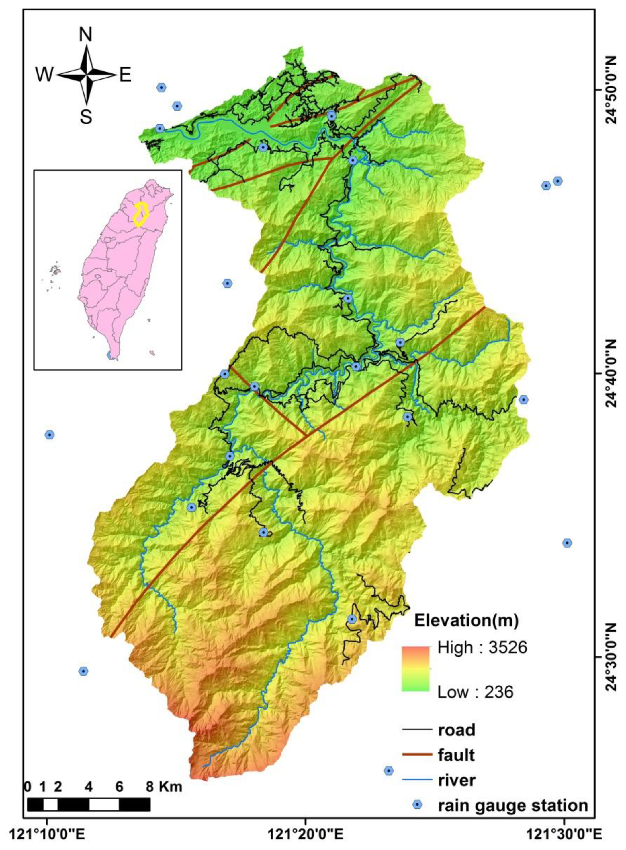
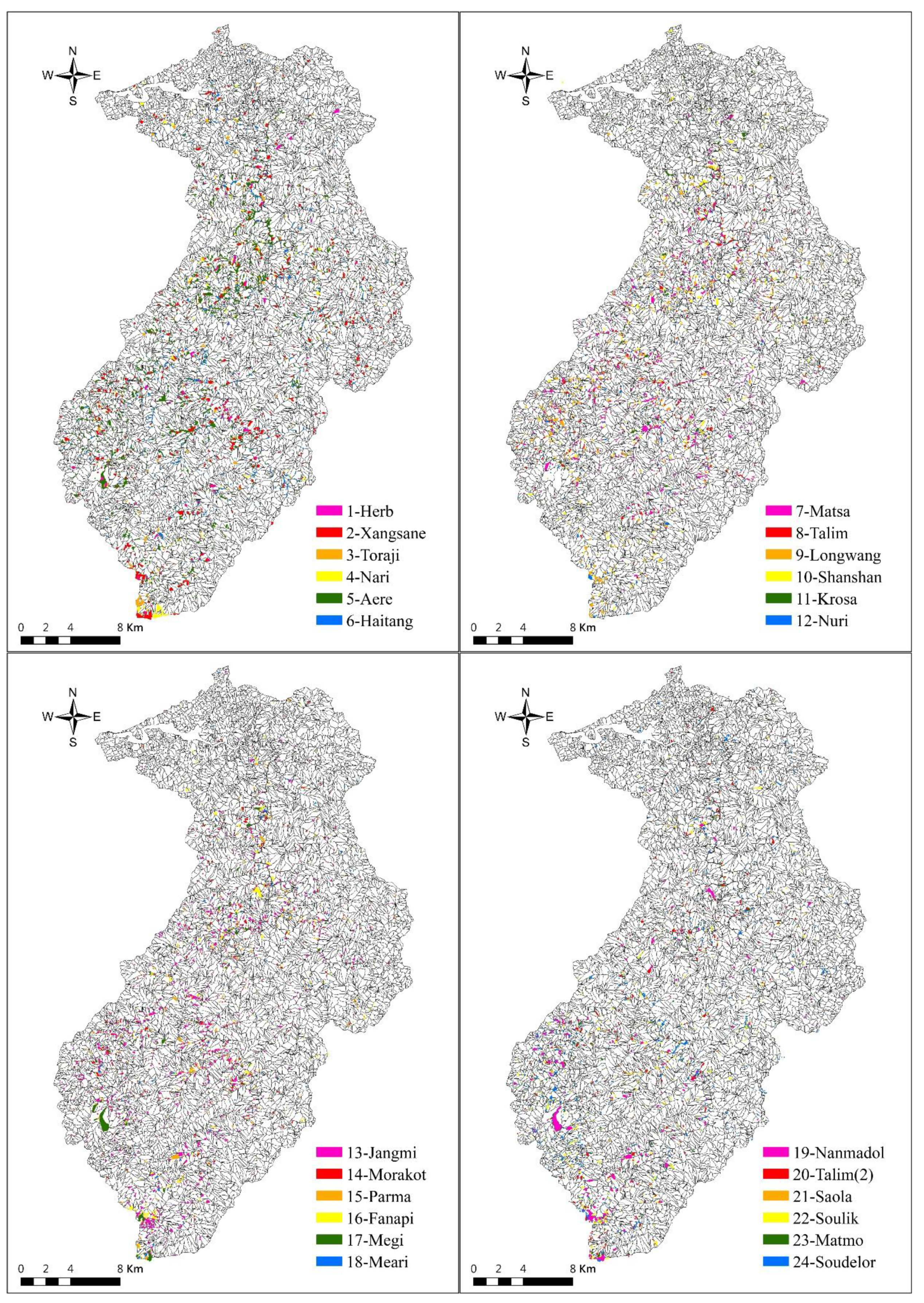
The Shihmen watershed, with an area of 75,243 ha, is located in the north part of Taiwan and is largely characterized by mountainous topography. Elevations in the area range from 236 m to 3526 m, and a slope gradient ranging from 20° to 50° accounts for 77% of the whole area (Figure 1). Because of the relatively well-defined topographic boundaries and topographic meaning in the Shihmen watershed, slope units were employed as analytical units for landslide susceptibility analysis. According to the subdivision method suggested by Xie et al. [52], this watershed was divided into 9181 slope units (Figure 2).

Figure 1. Elevation, road, fault, river system, and rain gauge station in the Shihmen watershed.

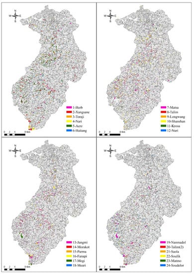
Figure 2. The slope units and landslide inventories, triggered by 24 typhoon events in the Shihmen watershed.

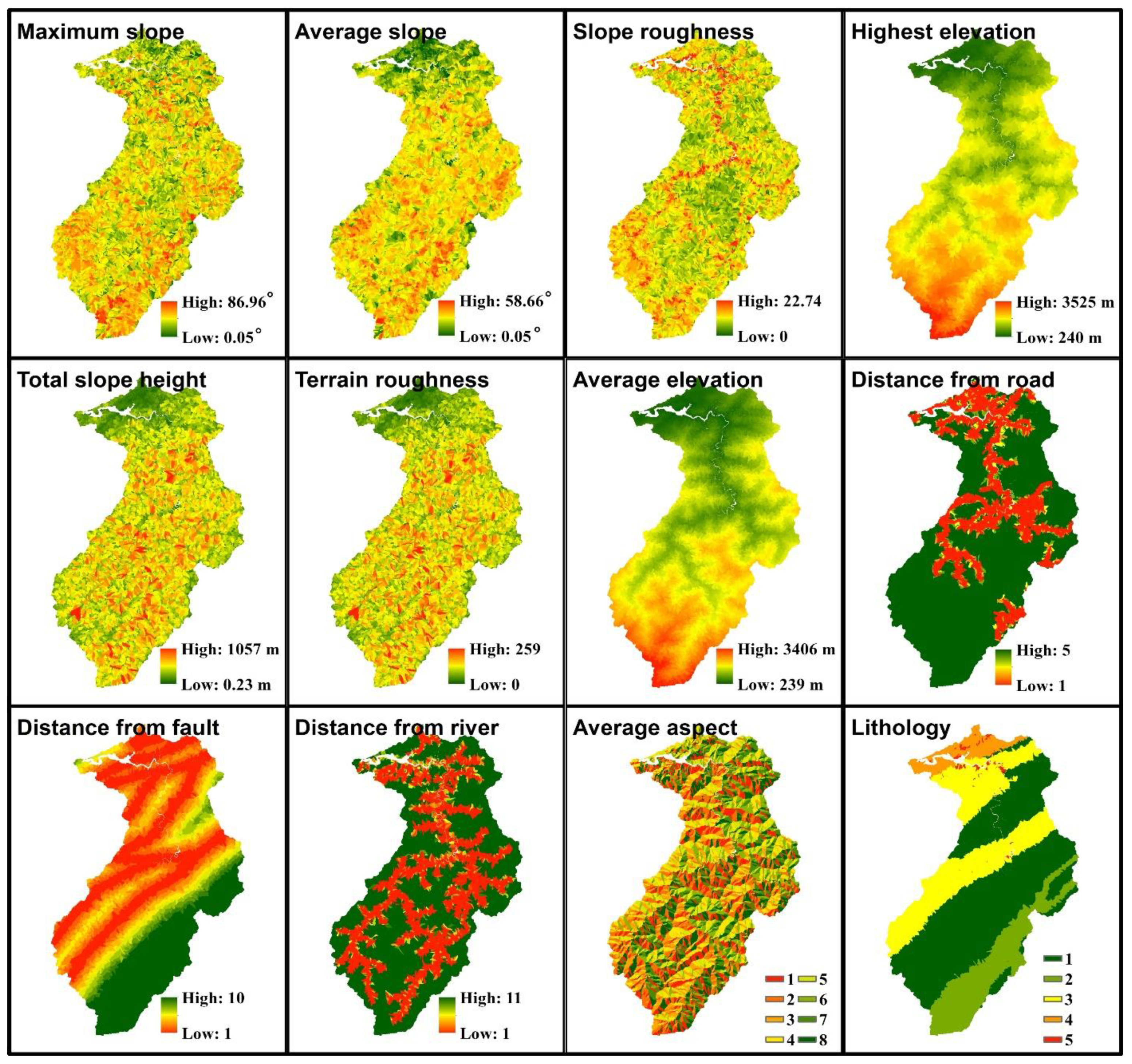
Twelve topographic factors, such as maximum slope, average slope, slope roughness, highest elevation, total slope height, terrain roughness, average elevation, distance from the road, distance from the fault, distance from the river, average aspect, and lithology, were selected as intrinsic susceptibility variables according to the previous study [6]. The values of highest elevation, total slope height, terrain roughness, average elevation, maximum slope, average slope, slope roughness, and average aspect of each slope unit were calculated by employing ArcGIS programs and by utilizing 5 m digital elevation model produced by the Ministry of the Interior. After obtaining the 1:5000 orthophoto base maps issued by the Aerial Survey Office of the Forestry Bureau, the 1:50,000 geologic maps issued by the Central Geological Survey and a road map overlay from the Soil and Water Conservation Bureau, we calculated the horizontal distances of each slope unit from the river, fault, and road, respectively. The lithologic types of each slope unit, such as argillite, quartzitic sandstone, hard sandstone and shale, sandstone and shale, and terrace deposit and alluvium, were analyzed utilizing the 1:50,000 geological maps. The distribution maps of 12 topographic factors are presented in Appendix A.

3.2. Landslide Inventory and Rainfall Factor

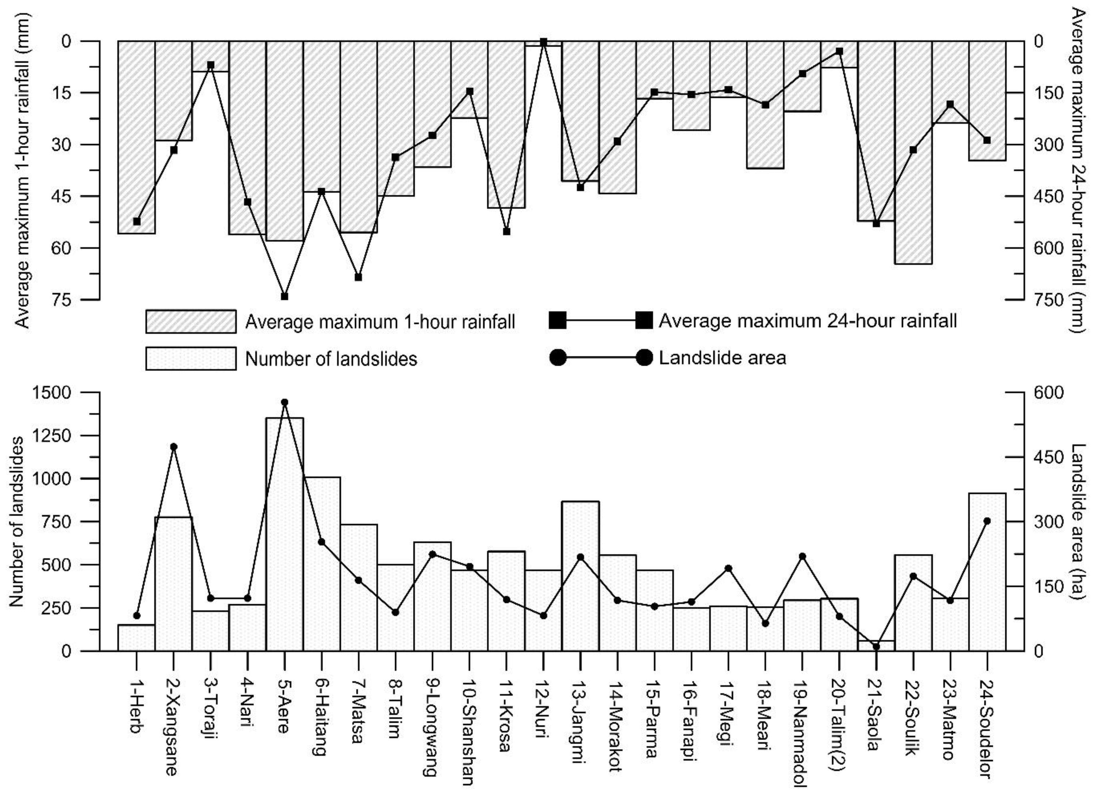
After collecting 24 sets of satellite images of the Shihmen watershed during the period from 1996 to 2015, landslide inventories triggered by 24 typhoon events were mapped according to the interpretation procedures proposed by Liu et al. [53]. The landslides recorded in the 24 landslide inventories in each slope unit are shown in Figure 2. The number of landslides for each landslide inventory ranged from 59 to 1350 and the total landslide area ranged from 10.19 ha to 577.04 ha (Figure 3).

Figure 3. Landslide inventory and rainfall statistics for 24 typhoon events.

Two rainfall factors, namely, maximum 1-h rainfall and maximum 24-h rainfall, were selected as extrinsic triggering variables, according to the previous research [6]. The short-duration rainfall and long-duration rainfall values reflect the rainfall pattern during the typhoon event. After collecting rainfall data from 31 rain-gauge stations (Figure 1), the maximum 1-h rainfall and maximum 24-h rainfall of each station during each typhoon event were analyzed. Then, the rainfall values of each slope unit were calculated, after using the Kriging method to estimate the spatial distribution of rainfall. The average maximum 1-h rainfall and maximum 24-h rainfall for each typhoon event are shown in Figure 3.

4. Results of Analysis

4.1. Results of Single Models

4.1.1. Logistic Regression (LR) Model

This study used LR to establish a parametric landslide susceptibility model. In the modeling process, 10-fold cross-validation was repeatedly used to assess model performance. The repeated application of this process reduced the sampling error and enabled the selection of the model with the best mean test accuracy for subsequent analysis. The test accuracy of 24 event-based logistic regression models (i.e., the AUROC value of the test stage) ranged from 0.740 to 0.862, and the mean accuracy was 0.819 (Table 4). Additionally, the test accuracy of the multi-year logistic regression model was 0.798.

Table 4. Performances of the LR models.

Event	Test Accuracy	Event	Test Accuracy
1-Herb	0.825	14-Morakot	0.832
2-Xangsane	0.776	15-Parma	0.802
3-Toraji	0.740	16-Fanapi	0.815
4-Nari	0.760	17-Megi	0.859
5-Aere	0.824	18-Meari	0.798
6-Haitang	0.789	19-Nanmadol	0.862
7-Matsa	0.832	20-Talim	0.812
8-Talim	0.806	21-Saola	0.815
9-Longwang	0.859	22-Soulik	0.835
10-Shanshan	0.826	23-Matmo	0.835
11-Krosa	0.850	24-Soudelor	0.823
12-Nuri	0.842	Multi-year	0.798
13-Jangmi	0.849

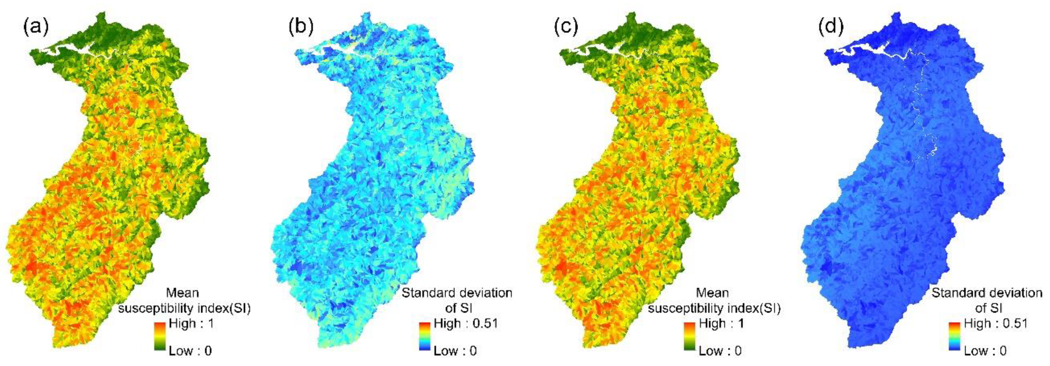
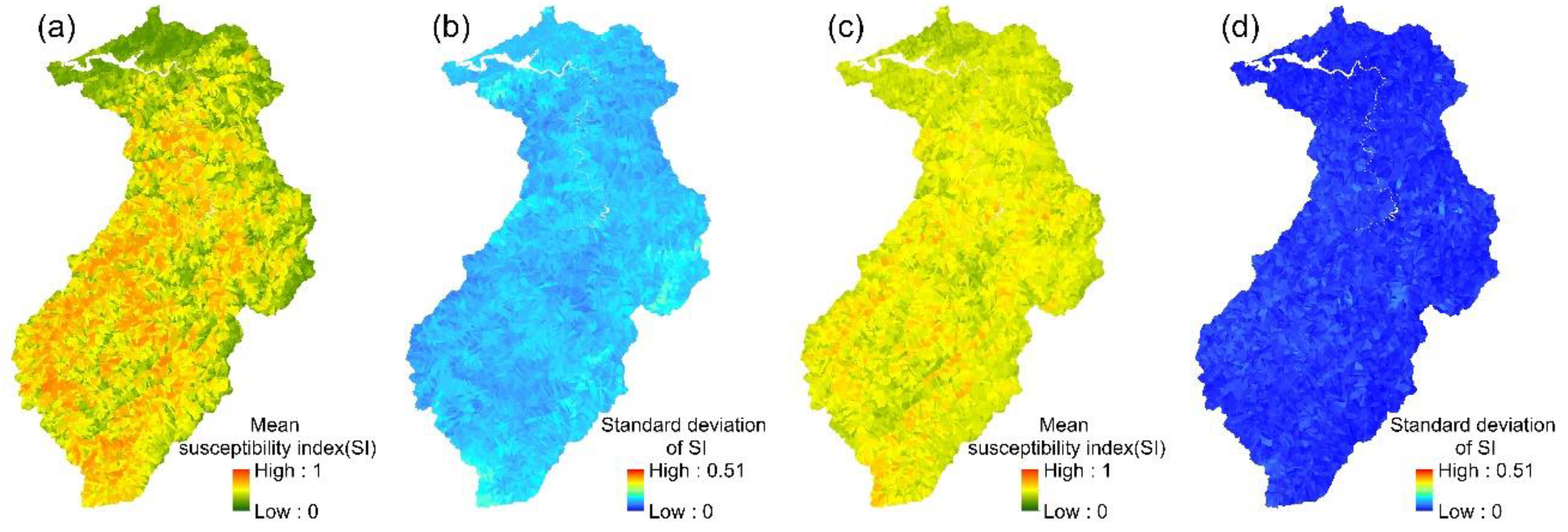
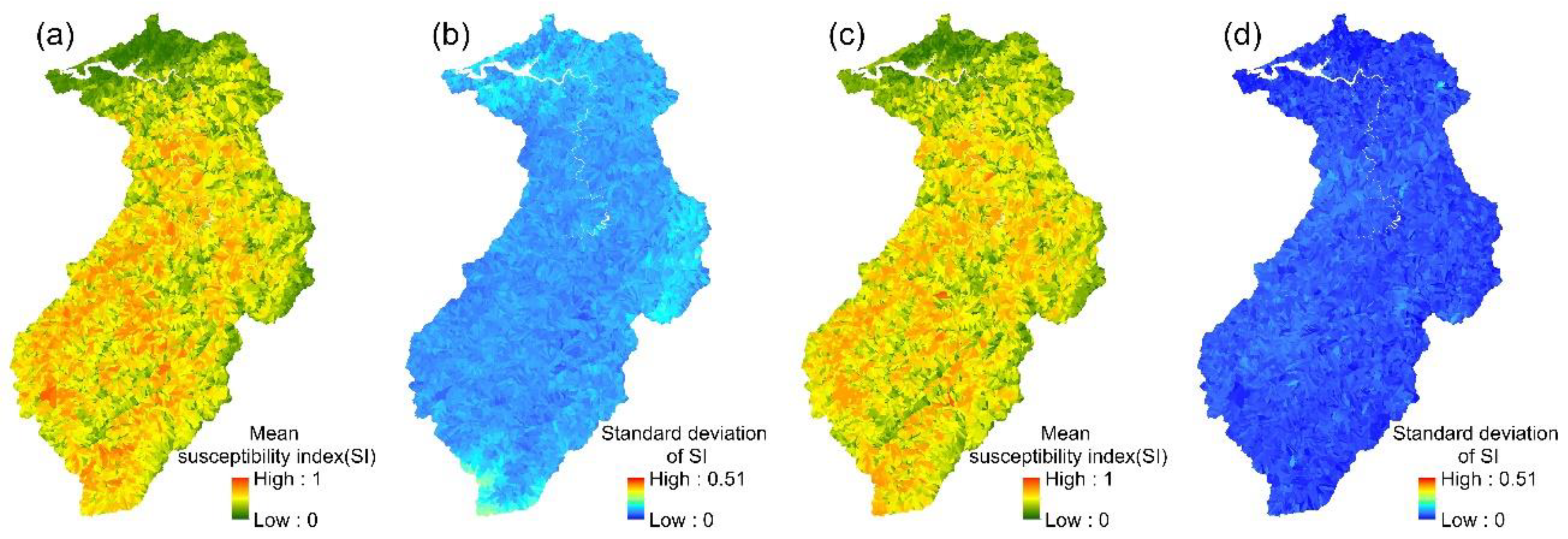
The 24 event-based logistic regression models established in this study enabled the spatial variation in each event’s landslide susceptibility index to be determined. The mean values and standard deviations of the 24 landslide susceptibility indices for each slope unit were then calculated (Figure 4). Similarly, the mean landslide susceptibility indices and standard deviations were calculated for each slope unit in the multi-year logistic regression model.

Figure 4. LR models: (a,b) the mean susceptibility index and standard deviation of 24 event-based models; (c,d) the mean susceptibility index and standard deviation of the multi-year model.

4.1.2. Random Forest (RF) Model

The hyperparameter tuning results for each event-based model, established using the RF algorithm, are shown in Table 5; it can be seen that the number of trees (numtree) ranged from 100 to 1000 and the number of variables (mtry) ranged from 7 to 14. The test accuracy of the 24 event-based models ranged from 0.772 to 0.944, and the mean was 0.842. Hyperparameter tuning for the multi-year RF model yielded a numtree: 400 and mtry: 14, and the model’s test accuracy was 0.789.

Table 5. The tuned hyperparameters and model performances for RF models.

Event	Hyperparameter Tuned		Test Accuracy	Event	Hyperparameter Tuned		Test Accuracy
	Numtree	Mtry			Numtree	Mtry
1-Herb	100	8	0.797	14-Morakot	300	13	0.815
2-Xangsane	500	14	0.772	15-Parma	1000	14	0.820
3-Toraji	700	11	0.851	16-Fanapi	600	14	0.848
4-Nari	400	13	0.821	17-Megi	200	11	0.872
5-Aere	1000	12	0.820	18-Meari	500	7	0.849
6-Haitang	700	11	0.792	19-Nanmadol	600	14	0.913
7-Matsa	700	12	0.845	20-Talim	600	13	0.824
8-Talim	300	11	0.808	21-Saola	700	13	0.944
9-Longwang	600	13	0.843	22-Soulik	500	11	0.846
10-Shanshan	500	14	0.819	23-Matmo	900	13	0.883
11-Krosa	700	12	0.855	24-Soudelor	400	13	0.827
12-Nuri	1000	14	0.881	Multi-year	400	14	0.789
13-Jangmi	900	13	0.855

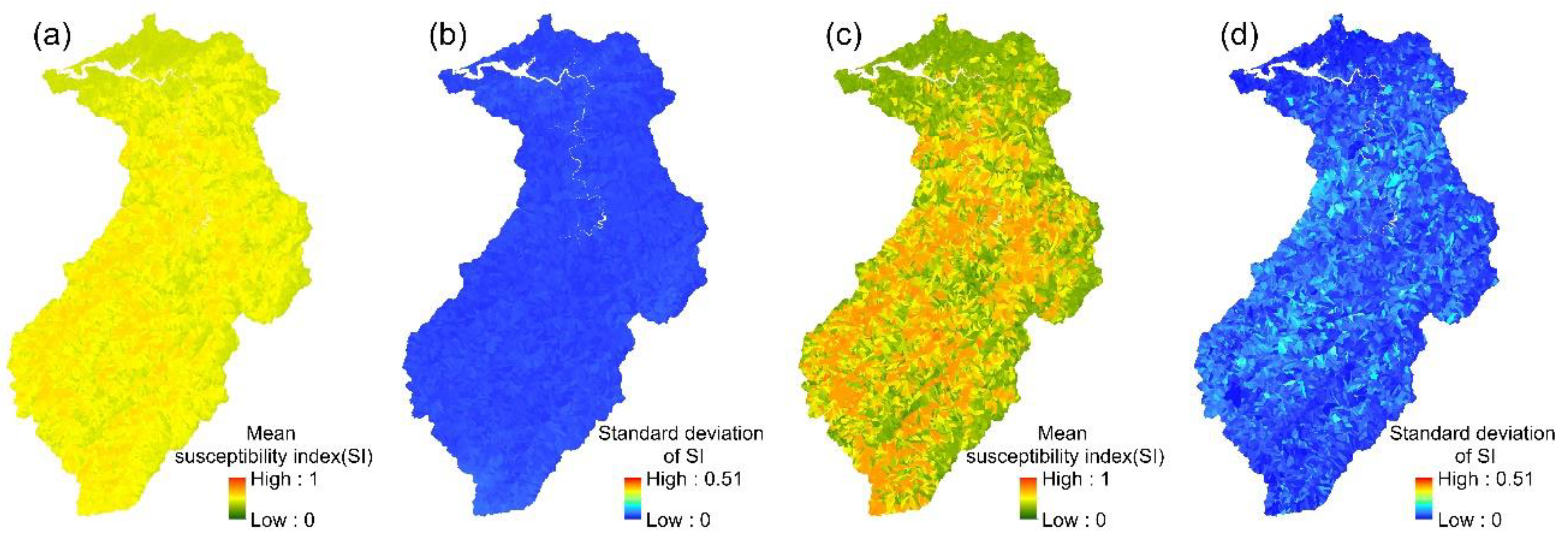
The spatial variation in each event’s landslide susceptibility index could be obtained from the 24 event-based RF models. The mean values and standard deviations of the 24 landslide susceptibility indices for each slope unit were then calculated (Figure 5). Similarly, the mean landslide susceptibility indices and standard deviations were calculated for each slope unit in the multi-year RF model.

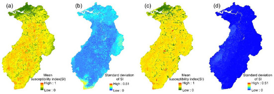
Figure 5. RF models: (a,b) the mean susceptibility index and standard deviation of 24 event-based models; (c,d) the mean susceptibility index and standard deviation of the multi-year model.

4.1.3. Support Vector Machine (SVM) Model

The hyperparameter tuning results for each event-based model, established using the SVM algorithm, are shown in Table 6; it can be seen that the penalty parameter (C) ranged from 0.029 to 754.312 and the RBF parameter (γ) ranged from 0.001 to 0.091. The test accuracy of all event-based models ranged from 0.674 to 0.861, and the mean was 0.754. Hyperparameter tuning for the multi-year SVM model yielded a penalty parameter (C) of 0.1 and an RBF parameter (γ) of 0.774, and the model’s test accuracy was 0.806.

Table 6. The tuned hyperparameters and model performances for SVM models.

Event	Hyperparameter Tuned		Test Accuracy	Event	Hyperparameter Tuned		Test Accuracy
	C	γ			C	γ
1-Herb	2.683	0.017	0.721	14-Morakot	0.029	0.029	0.768
2-Xangsane	79.060	0.007	0.717	15-Parma	2.024	0.052	0.766
3-Toraji	0.494	0.091	0.759	16-Fanapi	3.556	0.029	0.772
4-Nari	0.655	0.029	0.755	17-Megi	0.121	0.017	0.786
5-Aere	4.715	0.013	0.732	18-Meari	2.024	0.029	0.787
6-Haitang	33.932	0.001	0.729	19-Nanmadol	1.151	0.017	0.797
7-Matsa	754.312	0.001	0.757	20-Talim	4.715	0.002	0.674
8-Talim	2.024	0.069	0.758	21-Saola	10.985	0.091	0.861
9-Longwang	14.563	0.005	0.754	22-Soulik	19.307	0.002	0.712
10-Shanshan	138.950	0.002	0.741	23-Matmo	1.151	0.017	0.739
11-Krosa	2.024	0.007	0.758	24-Soudelor	0.373	0.007	0.728
12-Nuri	3.556	0.022	0.754	Multi-year	0.1	0.774	0.806
13-Jangmi	184.207	0.001	0.769

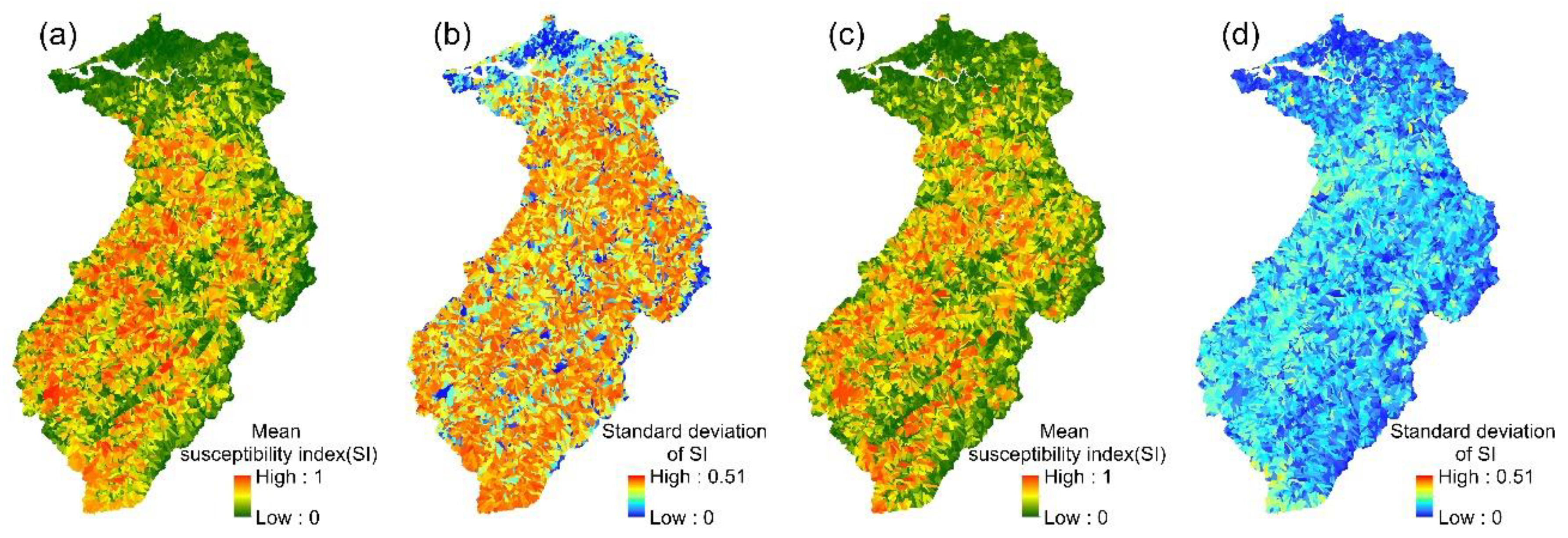
The spatial variation in each event’s landslide susceptibility index could be obtained from the 24 event-based SVM models. The mean values and standard deviations of the 24 landslide susceptibility indices for each slope unit were then calculated (Figure 6). Similarly, the mean landslide susceptibility indices and standard deviations were calculated for each slope unit in the multi-year SVM model.

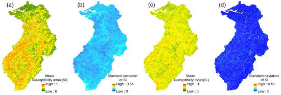
Figure 6. SVM models: (a,b) the mean susceptibility index and standard deviation of 24 event-based models; (c,d) the mean susceptibility index and standard deviation of the multi-year model.

4.1.4. Kernel Logistic Regression (KLR) Model

The hyperparameter tuning results for each event-based model established using the KLR algorithm are shown in Table 7; it can be seen that the penalty parameter (C) ranged from 0.017 to 244.205 and the RBF parameter (γ) ranged from 0.002 to 0.281. The test accuracy of every event-based model ranged from 0.712 to 0.833 and the mean was 0.754. Hyperparameter tuning for the multi-year KLR model yielded a penalty parameter (C) of 1.0 and an RBF parameter (γ) of 0.1; the model’s test accuracy was 0.812.

Table 7. The tuned hyperparameters and model performances for KLR models.

Event	Hyperparameter Tuned		Test Accuracy	Event	Hyperparameter Tuned		Test Accuracy
	C	γ			C	γ
1-Herb	244.205	0.005	0.712	14-Morakot	0.017	0.039	0.729
2-Xangsane	59.636	0.005	0.712	15-Parma	2.683	0.017	0.771
3-Toraji	1.151	0.052	0.781	16-Fanapi	33.932	0.013	0.784
4-Nari	10.985	0.017	0.775	17-Megi	2.024	0.069	0.815
5-Aere	1.151	0.022	0.760	18-Meari	33.932	0.007	0.725
6-Haitang	1.526	0.029	0.717	19-Nanmadol	8.286	0.003	0.829
7-Matsa	244.205	0.002	0.747	20-Talim	1.151	0.069	0.712
8-Talim	1.526	0.069	0.744	21-Saola	14.563	0.281	0.833
9-Longwang	3.556	0.039	0.765	22-Soulik	244.205	0.001	0.730
10-Shanshan	0.494	0.029	0.745	23-Matmo	1.526	0.039	0.737
11-Krosa	33.932	0.004	0.746	24-Soudelor	8.286	0.005	0.737
12-Nuri	59.636	0.029	0.723	Multi-year	1.0	0.1	0.812
13-Jangmi	3.556	0.029	0.767

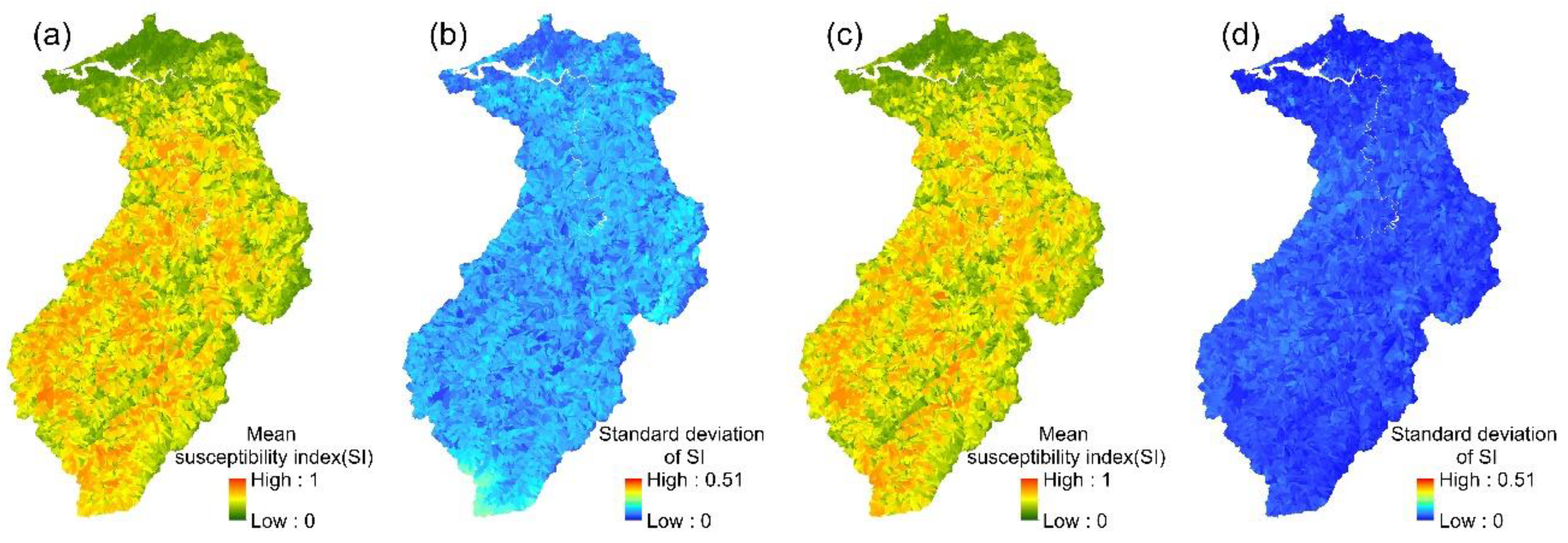
The spatial variation in each event’s landslide susceptibility index could be obtained from the 24 event-based KLR models. The mean values and standard deviations of the 24 landslide susceptibility indices for each slope unit were then calculated (Figure 7). Similarly, the mean landslide susceptibility indices and standard deviations were calculated for each slope unit in the multi-year KLR model.

Figure 7. KLR models: (a,b) the mean susceptibility index and standard deviation of 24 event-based models; (c,d) the mean susceptibility index and standard deviation of the multi-year model.

4.1.5. Gradient-Boosting Decision Tree (GBDT) Model

The hyperparameter tuning results for each event-based model established using the GBDT algorithm are shown in Table 8, and it can be seen that the number of trees (numtree) ranged from 100 to 1000, the number of variables (mtry) ranged from 6 to 14, and the learning rate ranged from 0.1 to 1.0. The test accuracy of the 24 event-based models ranged from 0.772 to 0.861 and the mean was 0.820. Hyperparameter tuning for the multi-year GBDT model yielded a numtree of 900, an mtry of 7, and a learning rate of 0.1; the model’s test accuracy was 0.804.

Table 8. The tuned hyperparameters and model performances for GBDT models.

Event	Hyperparameter Tuned			Test Accuracy	Event	Hyperparameter Tuned			Test Accuracy
	Numtree	Mtry	Learning Rate			Numtree	Mtry	Learning Rate
1-Herb	100	8	0.1	0.800	14-Morakot	200	8	0.1	0.833
2-Xangsane	700	13	0.9	0.772	15-Parma	300	13	0.5	0.823
3-Toraji	100	8	0.1	0.777	16-Fanapi	100	13	0.5	0.815
4-Nari	300	11	0.6	0.807	17-Megi	1000	13	0.8	0.848
5-Aere	600	14	0.3	0.821	18-Meari	1000	14	0.4	0.788
6-Haitang	200	11	0.7	0.772	19-Nanmadol	1000	10	0.7	0.852
7-Matsa	100	12	1.0	0.837	20-Talim	100	13	0.7	0.807
8-Talim	100	9	0.3	0.817	21-Saola	100	7	0.3	0.832
9-Longwang	200	6	0.1	0.845	22-Soulik	200	6	0.2	0.839
10-Shanshan	200	6	0.9	0.815	23-Matmo	100	6	1.0	0.843
11-Krosa	200	11	0.5	0.841	24-Soudelor	100	6	0.1	0.811
12-Nuri	1000	9	0.3	0.827	Multi-year	900	7	0.1	0.804
13-Jangmi	100	12	0.1	0.861

The spatial variation in each event’s landslide susceptibility index could be obtained from the 24 event-based GBDT models. The mean values and standard deviations of the 24 landslide susceptibility indices for each slope unit were then calculated (Figure 8). Similarly, the mean landslide susceptibility indices and standard deviations were calculated for each slope unit in the multi-year GBDT model.

Figure 8. GBDT models: (a,b) the mean susceptibility index and standard deviation of 24 event-based models; (c,d) the mean susceptibility index and standard deviation of the multi-year model.

4.2. Results of Ensemble Models

After establishing the single models, this study used the PM, PME, PMW, and CA ensemble methods to aggregate the landslide susceptibility indices of each single model for each event, yielding the landslide susceptibility indices of the 4 ensemble models.

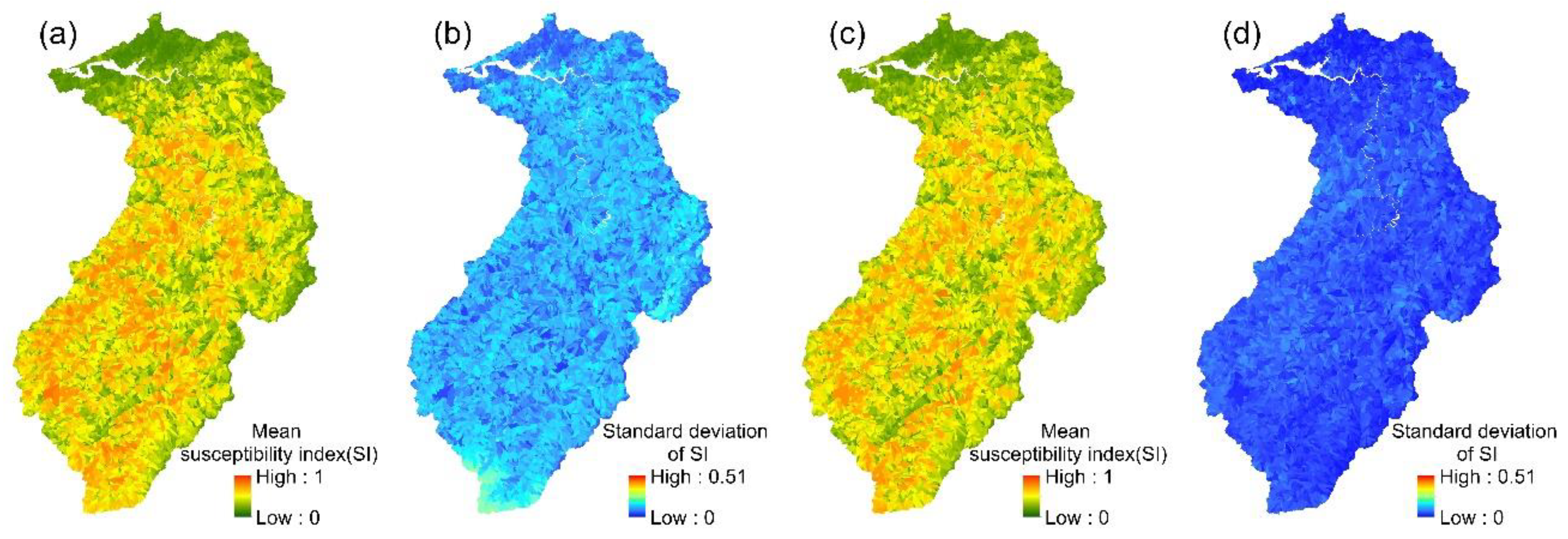
The spatial variation in each event’s landslide susceptibility index could be obtained from the 24 event-based PM ensemble models. The mean values and standard deviations of the 24 landslide susceptibility indices for each slope unit were then calculated (Figure 9). The mean landslide susceptibility indices and standard deviations that were calculated for each slope unit in the multi-year PM ensemble model are shown in Figure 9. Similarly, the mean susceptibility index and the standard deviation of the 24 event-based models, obtained using the PME, PMW, and CA ensemble methods, are shown in Figure 10, Figure 11 and Figure 12.

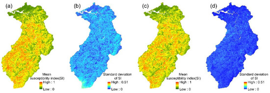
Figure 9. PM ensemble models: (a,b) the mean susceptibility index and standard deviation of 24 event-based models; (c,d) the mean susceptibility index and standard deviation of the multi-year model.

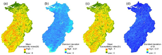
Figure 10. PME ensemble models: (a,b) the mean susceptibility index and standard deviation of 24 event-based models; (c,d) the mean susceptibility index and standard deviation of the multi-year model.

Figure 11. PMW ensemble models: (a,b) the mean susceptibility index and standard deviation of 24 event-based models; (c,d) the mean susceptibility index and standard deviation of the multi-year model.

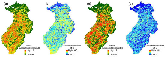
Figure 12. CA ensemble models: (a,b) the mean susceptibility index and standard deviation of 24 event-based models; (c,d) the mean susceptibility index and standard deviation of the multi-year model.

4.3. Assessment of Model Accuracy

After establishing all the above-mentioned models, this study assessed the predictive ability of each model established using a specific landslide inventory by examining that model’s ability to predict the remaining landslide events. For the sake of clarity, the section below will employ the terminology $a_{i,j,k}$ to indicate the accuracy of the various models established using different landslide inventories and different modeling methods. Here, i = 1–25 indicate the individual landslide inventories used in modeling, where 1–24 are event-based landslide inventories, and 25 is the multi-year landslide inventory; j = 1–24 indicate the predicted events; and k = 1–9 indicate the different modeling methods.

The accuracy of each PM ensemble model is shown in Table 9; AUROC > 75% is indicated in green, AUROC 75–50% is indicated in yellow, and AUROC < 50% is indicated in red. The average predictive accuracy of event-based models (i = 1–24, j = 1–24, i ≠ j, k = 6) ranged from 70.9% to 77.9% and the mean was 74.8%; the average predictive accuracy of the multi-year model (i = 25, j = 1–24, k = 6) was 91.1%. The average predictive accuracy of the LR models (k = 1), RF models (k = 2), SVM models (k = 3), KLR models (k = 4), GBDT models (k = 5), PME ensemble models (k = 7), PMW ensemble models (k = 8), and CA ensemble models (k = 9) were also obtained.

Table 9. AUROCs (%) of each PM ensemble model for the calibration or prediction of other landslide events. AUROC > 75% is indicated in green, AUROC 75–50% is indicated in yellow.

		Event for Calibration or Prediction
		1	2	3	4	5	6	7	8	9	10	11	12	13	14	15	16	17	18	19	20	21	22	23	24
Model trained by event	1	90	71	70	67	79	67	75	74	76	77	75	77	78	75	76	75	78	76	78	73	74	69	76	67
	2	74	90	75	78	71	74	70	76	81	79	78	78	75	73	79	79	83	76	81	75	80	73	78	77
	3	70	75	92	75	71	74	73	74	78	78	76	74	79	75	77	77	81	74	81	72	78	76	78	74
	4	71	75	72	92	65	71	67	70	77	76	78	75	77	69	77	76	79	68	79	70	80	69	73	72
	5	80	77	74	74	91	74	81	78	81	82	78	79	83	79	77	78	83	78	82	74	73	75	80	72
	6	67	73	69	74	70	90	76	82	75	77	78	78	78	76	76	72	79	76	77	74	79	76	75	72
	7	72	73	68	69	79	76	91	78	77	76	79	77	78	77	76	72	76	72	77	70	76	72	72	70
	8	64	70	65	65	73	74	72	91	75	74	76	78	70	73	72	67	68	75	77	72	65	72	72	68
	9	76	75	72	75	78	75	76	78	93	79	82	80	78	74	78	77	78	78	84	75	79	78	80	79
	10	76	75	74	75	80	72	76	75	82	90	80	80	81	77	79	77	84	77	79	73	77	76	79	73
	11	74	74	67	74	74	74	76	77	81	79	92	74	79	77	78	71	79	73	69	68	75	67	69	71
	12	71	70	70	71	72	70	72	72	75	73	73	90	74	71	74	77	79	73	76	70	77	72	76	72
	13	77	77	74	76	78	75	80	79	78	79	82	75	92	79	77	75	75	74	76	71	82	79	77	64
	14	72	70	66	68	78	72	79	78	76	78	78	78	77	90	74	69	76	77	70	71	69	68	73	65
	15	69	76	72	77	69	69	68	68	80	81	78	82	74	69	91	77	84	73	82	75	77	67	77	77
	16	67	71	71	69	74	66	72	63	71	74	74	72	70	69	73	93	81	69	69	67	77	63	76	74
	17	72	73	73	74	76	63	71	69	79	79	72	79	71	75	78	78	93	74	81	73	70	73	76	78
	18	72	71	69	69	68	72	70	74	79	77	71	78	73	71	76	72	74	89	80	75	79	77	79	78
	19	72	72	70	74	74	74	76	74	78	77	72	79	74	72	78	74	81	73	93	74	83	79	80	77
	20	69	70	63	68	71	73	72	73	76	73	71	79	72	70	70	72	75	75	79	89	80	74	76	74
	21	66	74	70	72	69	74	73	75	76	77	74	79	80	73	76	74	80	73	81	73	91	79	77	75
	22	72	72	67	72	75	73	74	76	77	77	71	80	80	76	74	72	78	80	85	75	83	92	81	79
	23	72	73	70	71	76	71	72	73	79	78	73	79	76	75	75	76	80	77	82	74	75	80	92	81
	24	74	74	69	72	75	75	75	77	82	80	77	81	77	77	78	76	83	80	82	76	80	81	82	89
	25	90	88	89	90	92	89	92	90	92	91	91	94	93	90	91	89	94	91	95	91	92	93	92	89

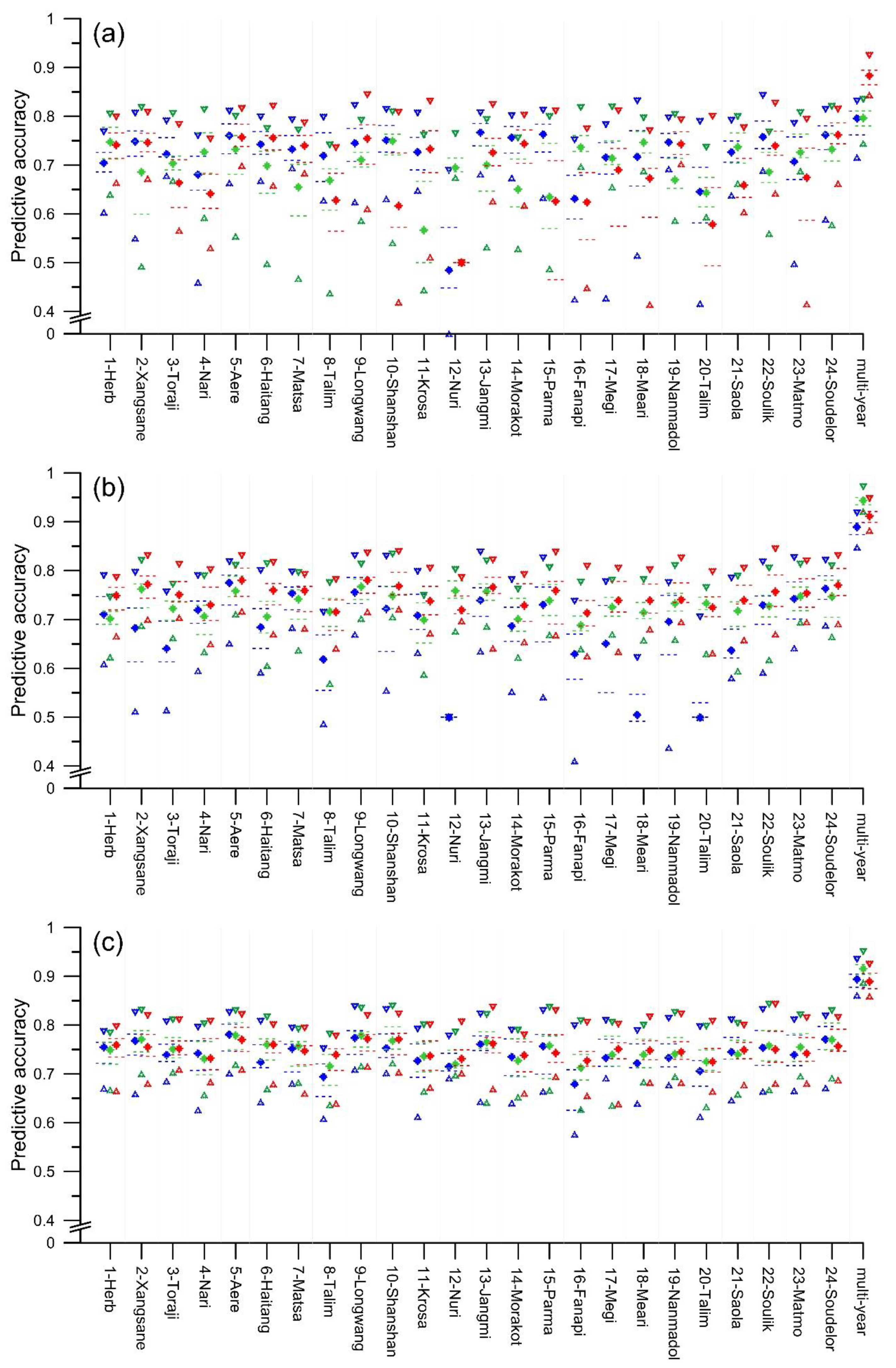
The average predictive accuracy of the 5 event-based single landslide susceptibility models (k = 1–5) with regard to the other landslide events is shown in Figure 13. In Figure 13, from top down, the various symbols represent the maximum, third quartile, median, first quartile, and minimum of a box plot of average predictive accuracy. This figure also shows the predictive accuracy distribution of the multi-year single landslide susceptibility models. In particular, the average predictive accuracy of the event-based LR models (i = 1–24, j = 1–24, i ≠ j, k = 1) ranged from 48.8% to 76.1%, and the mean was 71.2%; the multi-year LR model had a mean predictive accuracy of 78.8%. Similarly, the average predictive accuracy of event-based RF models ranged from 57.9% to 74.7%, and the mean was 69.5%; the multi-year RF model had a mean predictive accuracy of 79.5%. The average predictive accuracy of event-based SVM models ranged from 50.0% to 76.1%, and the mean was 68.1%; the multi-year SVM model had a mean predictive accuracy of 88.0%. The average predictive accuracy of event-based KLR models ranged from 50.0% to 76.4% and the mean was 67.4%; the multi-year KLR model had a mean predictive accuracy of 88.6%. The average predictive accuracy of event-based GBDT models ranged from 69.2% to 76.3%, while the mean was 72.8%; the multi-year GBDT model had a mean predictive accuracy of 94.3%.

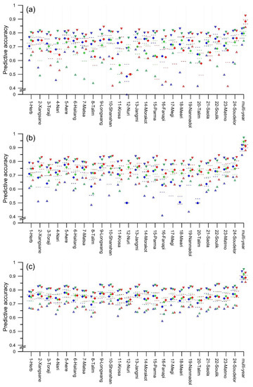
Figure 13. Box plot of the average predictive accuracy of single and ensemble models in the prediction of other landslide events: (a) blue, green, and red represent LR, RF, and SVM, respectively; (b) blue, green, and red represent KLR, GBDT, and PM, respectively; (c) blue, green, and red represent PME, PMW, and CA, respectively.

The average predictive accuracy of the 4 event-based ensemble landslide susceptibility models (k = 6–9) with regard to the other landslide events is shown in Figure 13, which also shows the predictive accuracy distribution of the multi-year ensemble landslide susceptibility models. In Figure 13, the average predictive accuracy of event-based PME models (i = 1–24, j = 1–24, i ≠ j, k = 7) ranged from 67.0% to 77.5% and the mean was 73.8%; the multi-year PME model had a mean predictive accuracy of 89.2%. The average predictive accuracy of event-based PMW models ranged from 70.9% to 77.8%, and the mean was 74.7%; the multi-year PMW model had a mean predictive accuracy of 91.6%. The average predictive accuracy of event-based CA models ranged from 72.7% to 77.1%, while the mean was 74.8%; the mean predictive accuracy of the multi-year CA model was 89.0%. These results indicate that the event-based ensemble models all had an AUROC > 50% with regard to other landslide events (i = 1–24, j = 1–24, i ≠ j, k = 6–9).

5. Discussion

5.1. Comparison of the Performance of Single and Ensemble Models

It can be seen from Figure 13 that the predictive accuracy of the ensemble models is superior to that of single models under most circumstances. In particular, the four ensemble models established on the basis of event-based landslide inventories 1, 3, 4, 9, 10, 17, and 21, as well as the multi-year landslide inventory all had greater predictive accuracy than any single models. In addition, the four ensemble models established on the basis of the event-based landslide inventories 2, 5, 7, 11, 12, 13, 15, 16, 18, 20, and 22 had greater predictive accuracy than at least any four single models. In other words, when establishing a model using the same landslide inventory, most ensemble models will offer superior predictive accuracy.

The mean predictive accuracy of different modeling methods (k = 1–9) are compared in Table 10. It can be seen that the mean predictive accuracy of ensemble models (k = 6–9) ranged from 0.738 to 0.748 and was higher than the accuracy range of 0.674–0.728 for single models (k = 1–5). Since the Kolmogorov–Smirnov test indicated that not all datasets were normally distributed, the Kruskal–Wallis test was used to compare the predictive accuracy of different modeling methods (Table 11). The post hoc test indicated that the predictive accuracy of ensemble models is consistently superior to that of single models. Furthermore, the coefficient of variation (CV) of the predictive accuracy of ensemble models ranged from 0.047 to 0.063, which was lower than the CV range for single models. In summary, our results show that ensemble landslide susceptibility models offer superior predictive ability and relatively low uncertainty.

Table 10. Performance assessment of the different modeling methods.

Inventory Type	Metric	LR(1)	RF(2)	SVM(3)	KLR(4)	GBDT(5)	PM(6)	PME(7)	PMW(8)	CA(9)
Event-based	Mean training accuracy	0.813	0.878	0.833	0.856	0.977	0.909	0.883	0.912	0.923
	CV of training accuracy	0.038	0.028	0.054	0.037	0.011	0.013	0.017	0.013	0.019
	Mean predictive accuracy	0.712	0.695	0.681	0.674	0.728	0.748	0.738	0.747	0.748
	CV of predictive accuracy	0.118	0.104	0.146	0.142	0.059	0.055	0.063	0.055	0.047
Multi-year	Mean predictive accuracy	0.788	0.795	0.880	0.886	0.943	0.911	0.892	0.916	0.890
	CV of predictive accuracy	0.040	0.029	0.026	0.021	0.014	0.019	0.022	0.018	0.022

Table 11. Kruskal–Wallis test of the predictive accuracy of different modeling methods.

	N	Mean Rank	d.f.	H	p	Post Hoc Test
LR(1)	576	2481.79	8	514.142	0.000	>2–4
RF(2)	576	2013.05				-
SVM(3)	576	2080.67				-
KLR(4)	576	1924.60				-
GBDT(5)	576	2571.61				>2–4
PM(6)	576	3134.95				>1–5
PME(7)	576	2873.52				>1–5
PMW(8)	576	3120.86				>1–5
CA(9)	576	3131.45				>1–5

Prior studies have demonstrated that the predictive ability of the landslide susceptibility models established by different ensemble methods was superior to that of single landslide susceptibility models [16,31,34,35]. In accordance with the previous study results, we found that most ensemble models were superior in terms of predictive accuracy to the single models developed with the same inventory. Moreover, this study used 24 inventories to establish the corresponding ensemble models. The higher predictive ability of the ensemble models for each inventory implied that the PM, PME, PMW, and CA ensemble methods were robust for enhancing the predictive performance of landslide susceptibility models in the study area.

Among the single models, while LR models had the lowest mean training accuracy (i = 1–24, j = 1–24, i = j, k = 1), their mean predictive accuracy of 0.712 (i = 1–24, j = 1–24, i ≠ j, k = 1) was higher than that of the RF, SVM, and KLR models. Although the RF, SVM, and KLR models had very good mean training accuracy, their mean predictive accuracy was poor; this may be because these nonparametric models require a greater quantity of data for training and are prone to overfitting [2,8].

5.2. Comparison of the Performance of Event-Based and Multi-Year Models

It can be seen from Figure 13 that among the nine modeling methods, the predictive accuracy of multi-year models is consistently superior to that of the 24 event-based models. Table 10 also reveals that the mean predictive accuracy of multi-year models (i = 25, j = 1–24) ranged from 0.788 to 0.943, which was higher than the values of 0.674–0.748 in the event-based models (i = 1–24, j = 1–24, i ≠ j). The results of the Mann–Whitney U test (Table 12) indicate that among the nine modeling methods, the predictive performance of models established based on multi-year landslide inventories is uniformly superior to that of event-based models. Furthermore, the CV of the multi-year models’ predictive accuracy (0.014–0.040) was lower than that of event-based models. In summary, multi-year landslide susceptibility models offer excellent predictive performance and low uncertainty.

Table 12. Mann–Whitney U test of the predictive accuracy of models, based on different types of landslide inventories.

Modeling Method	Inventory Type	N	Mean Rank	Sum of	U	p
LR (1)	Event-based	552	279.95	154,531.00	1903.000	0.000
	Multi-year	24	485.21	11,645.00
RF (2)	Event-based	552	277.78	153,332.00	704.000	0.000
	Multi-year	24	535.17	12,844.00
SVM (3)	Event-based	552	276.50	152,629.00	1.000	0.000
	Multi-year	24	564.46	13,547.00
KLR (4)	Event-based	552	276.50	152,628.00	0.000	0.000
	Multi-year	24	564.50	13,548.00
GBDT (5)	Event-based	552	276.50	152,628.00	0.000	0.000
	Multi-year	24	564.50	135,48.00
PM (6)	Event-based	552	276.50	152,628.00	0.000	0.000
	Multi-year	24	564.50	13,548.00
PME (7)	Event-based	552	276.50	152,628.00	0.000	0.000
	Multi-year	24	564.50	13,548.00
PMW (8)	Event-based	552	276.50	152,628.00	0.000	0.000
	Multi-year	24	564.50	13,548.00
CA (9)	Event-based	552	276.50	152,628.00	0.000	0.000
	Multi-year	24	564.50	13,548.00

The findings of the current study that the relatively excellent predictive performance and low uncertainty of the landslide susceptibility models established using multi-year landslide inventories verifies the advantage of using a combination of event-based inventories and confirms the previous study results. The relatively high predictive abilities of the landslide susceptibility models, built by the combination of different event-based landslide inventories, have been thought to be related to their bigger landslide sample size and the wider numerical range of rainfall parameters in the training sample [23,54,55], or to their lower concentration of landslides in areas with the same lithology and a lower collinearity between rainfall parameters and lithology [56,57].

It can also be seen from Figure 13 that when applying the same modeling method, the predictive accuracy of event-based models depends on the choice of event. For example, in terms of the average predictive accuracy of the 24 event-based LR models, a maximum of 76.1% appeared when employing the event in Jangmi, and a minimum of 48.8% was obtained when using the event in Nuri, while the range is 27.30%. Similarly, the ranges of the average predictive accuracy of the 24 event-based RF, SVM, KLR, GBDT, PM, PME, PMW, and CA models are 16.80%, 26.10%, 26.40%, 7.10%, 7.00%, 10.50%, 6.90%, and 4.40%, respectively. These results confirmed the findings of previous studies that the choice of event has an influence on the predictive ability of the event-based landslide susceptibility model established [22,23,24], which may correlate with the event’s rainfall intensity range [3] and the event’s spatial concentration degree of landslides [56,57].

5.3. Correlations between the Susceptibility Maps of the Optimal Model and Other Models

It can be seen from Figure 4, Figure 5, Figure 6, Figure 7, Figure 8, Figure 9, Figure 10, Figure 11 and Figure 12 that when a specific modeling method is used, the high susceptibility areas in landslide susceptibility maps, based on multi-year models, are similar to those created using the mean susceptibility indices of 24 event-based models. Nevertheless, there are significant differences in the landslide susceptibility index range and standard deviation among the different modeling methods. Because PM ensemble models have optimal predictive accuracy (Table 11) and multi-year models are superior to event-based models (Table 12), this study considered the multi-year PM ensemble model to be the optimal landslide susceptibility model. This model’s landslide susceptibility map is the most representative and can best reflect the probabilities of landslides in different slope units of the research area.

We also compared these landslide susceptibility maps, in order to analyze the correlations in the spatial distribution of susceptibility index between the multi-year PM ensemble model and other models. Rather than performing the mutual subtraction algorithm [6,58,59,60] or the histogram matching method [55,56], we calculated the Spearman’s rank correlation coefficient to assess the degree of difference between the susceptibility maps of the optimal model and other models. As shown in Table 13, the correlation coefficient of the single models ranged from 0.811 to 0.946, with an average of 0.912, which was lower than the 0.940–1.00 correlation coefficient range of the ensemble models. This indicates that there are only relatively small differences between the susceptibility maps of the optimal model and other ensemble models. In addition, when a multi-year landslide inventory is not available, the fact that the average correlation coefficient of the single models was lower than the average correlation coefficient of the ensemble models indicates that ensemble models can effectively reduce the discrepancies between the susceptibility maps of the established models and the optimal model.

Table 13. Degree of difference between the susceptibility maps of the multi-year PM ensemble model and other models.

Susceptibility Map	Spearman’s Rank Correlation Coefficient	Susceptibility Map	Spearman’s Rank Correlation Coefficient
Event-based LR model	0.924	Multi-year LR model	0.928
Event-based RF model	0.917	Multi-year RF model	0.913
Event-based SVM model	0.938	Multi-year SVM model	0.811
Event-based KLR model	0.946	Multi-year KLR model	0.864
Event-based GBDT model	0.938	Multi-year GBDT model	0.936
Event-based PM ensemble model	0.962	Multi-year PM ensemble model	1.000
Event-based PME ensemble model	0.954	Multi-year PME ensemble model	0.990
Event-based PMW ensemble model	0.963	Multi-year PMW ensemble model	1.000
Event-based CA ensemble model	0.940	Multi-year CA ensemble model	0.950

6. Conclusions

This study collected 24 event-based landslide inventories for the Shihmen watershed and employed logistic regression, random forest, support vector machine, kernel logistic regression, and gradient boosting decision tree methods to establish event-based single landslide susceptibility models. We also used four ensemble methods to aggregate the results of single models, to establish event-based ensemble models. In addition, the 24 event-based landslide inventories were combined to form a multi-year landslide inventory, which was used to establish multi-year single landslide susceptibility models and multi-year ensemble models.

As shown in Table 10, Table 11 and Table 12, the current study found that an ensemble model based on a multi-year inventory can achieve excellent predictive accuracy. Compared with event-based models, multi-year landslide susceptibility models offer superior predictive ability and lower uncertainty; compared with single models, ensemble landslide susceptibility models have higher predictive ability and lower uncertainty for each inventory, implying that the four ensemble methods are robust for enhancing the model’s predictive performance in the study area.

When relying on an event-based landslide inventory instead of a multi-year inventory to establish a model, the predictive accuracy of single models has considerable uncertainty due to differences in the predicted landslide events. The ensemble models can both reduce uncertainty and achieve better predictive accuracy, while the established PM ensemble models are the most effective of all. The susceptibility map created using the 24 PM ensemble models, based on different event-based landslide inventories, revealed areas where landslides are likely to occur. High-priority landslide mitigation measures should be implemented in places with a high mean susceptibility index and a low variation in susceptibility index to effectively reduce the losses caused by the landslides.

We recommend that other modeling methods, such as neural networks and deep learning, be further employed to establish landslide susceptibility models. When there are large numbers of single models, other ensemble methods, such as the confidence interval of the mean susceptibility index, may be used to establish even more effective ensemble landslide susceptibility models. Finally, due to the influence of the choice of event on the predictive ability of an event-based model and the better predictive ability of the models built by the combination of different event-based landslide inventories, future research can investigate possible improvements in predictive ability by combining two different event-based inventories to create an ensemble model when researchers are lacking a multi-year inventory.

References

- Van Westen, C.; Van Asch, T.W.; Soeters, R. Landslide hazard and risk zonation—Why is it still so difficult? Bull. Eng. Geol. Environ. 2006, 65, 167–184. [Google Scholar] [CrossRef]
- Brownlee, J. Parametric and Nonparametric Machine Learning Algorithms. Machine Learning Mastery. Available online: https://machinelearningmastery.com/parametric-and-nonparametric-machine-learning-algorithms (accessed on 12 January 2021).
- Lee, C.T.; Huang, C.C.; Lee, J.F.; Pan, K.L.; Lin, M.L.; Dong, J.J. Statistical approach to storm event-induced landslides susceptibility. Nat. Hazards Earth Syst. Sci. 2008, 8, 941–960. [Google Scholar] [CrossRef] [Green Version]
- Lu, A.; Haung, W.K.; Lee, C.F.; Wei, L.W.; Lin, H.H.; Chi, C. Combination of Rainfall Thresholds and Susceptibility Maps for Early Warning Purposes for Shallow Landslides at Regional Scale in Taiwan. In Workshop on World Landslide Forum; Casagli, N., Tofani, V., Sassa, K., Bobrowsky, P.T., Takara, K., Eds.; Springer: Cham, Germany, 2020; pp. 217–225. [Google Scholar]
- Rossi, M.; Guzzetti, F.; Reichenbach, P.; Mondini, A.C.; Peruccacci, S. Optimal landslide susceptibility zonation based on multiple forecasts. Geomorphology 2010, 114, 129–142. [Google Scholar] [CrossRef]
- Wu, C.Y.; Chen, S.C. Integrating spatial, temporal, and size probabilities for the annual landslide hazard maps in the Shihmen watershed, Taiwan. Nat. Hazards Earth Syst. Sci. 2013, 13, 2353–2367. [Google Scholar] [CrossRef] [Green Version]
- Wu, C. Landslide Susceptibility Based on Extreme Rainfall-Induced Landslide Inventories and the Following Landslide Evolution. Water 2019, 11, 2609. [Google Scholar] [CrossRef] [Green Version]
- Zhao, L.; Wu, X.; Niu, R.; Wang, Y.; Zhang, K. Using the rotation and random forest models of ensemble learning to predict landslide susceptibility. Geomat. Nat. Hazards Risk 2020, 11, 1542–1564. [Google Scholar] [CrossRef]
- Brock, J.; Schratz, P.; Petschko, H.; Muenchow, J.; Micu, M.; Brenning, A. The performance of landslide susceptibility models critically depends on the quality of digital elevation models. Geomat. Nat. Hazards Risk 2020, 11, 1075–1092. [Google Scholar] [CrossRef]
- Bui, D.T.; Le, K.T.T.; Nguyen, V.C.; Le, H.D.; Revhaug, I. Tropical forest fire susceptibility mapping at the Cat Ba National Park Area, Hai Phong City, Vietnam, using GIS-based kernel logistic regression. Remote Sens. 2016, 8, 347. [Google Scholar] [CrossRef] [Green Version]
- Bui, D.T.; Tuan, T.A.; Klempe, H.; Pradhan, B.; Revhaug, I. Spatial prediction models for shallow landslide hazards: A comparative assessment of the efficacy of support vector machines, artificial neural networks, kernel logistic regression, and logistic model tree. Landslides 2016, 13, 361–378. [Google Scholar]
- Chang, K.T.; Merghadi, A.; Yunus, A.P.; Pham, B.T.; Dou, J. Evaluating scale effects of topographic variables in landslide susceptibility models using GIS-based machine learning techniques. Sci. Rep. 2019, 9, 12296. [Google Scholar] [CrossRef] [Green Version]
- Mokhtari, M.; Abedian, S. Spatial prediction of landslide susceptibility in Taleghan basin, Iran. Stoch. Environ. Res. Risk Assess. 2019, 33, 1297–1325. [Google Scholar] [CrossRef]
- Oh, H.J.; Kadavi, P.R.; Lee, C.W.; Lee, S. Evaluation of landslide susceptibility mapping by evidential belief function, logistic regression and support vector machine models. Geomat. Nat. Hazards Risk 2018, 9, 1053–1070. [Google Scholar] [CrossRef] [Green Version]
- Schratz, P.; Muenchow, J.; Iturritxa, E.; Richter, J.; Brenning, A. Hyperparameter tuning and performance assessment of statistical and machine-learning algorithms using spatial data. Ecol. Model. 2019, 406, 109–120. [Google Scholar] [CrossRef] [Green Version]
- Kim, H.G.; Lee, D.K.; Park, C.; Ahn, Y.; Kil, S.H.; Sung, S.; Biging, G.S. Estimating landslide susceptibility areas considering the uncertainty inherent in modeling methods. Stoch. Environ. Res. Risk Assess. 2018, 32, 2987–3019. [Google Scholar] [CrossRef]
- Park, S.; Kim, J. Landslide susceptibility mapping based on random forest and boosted regression tree models, and a comparison of their performance. Appl. Sci. 2019, 9, 942. [Google Scholar] [CrossRef] [Green Version]
- Nsengiyumva, J.B.; Valentino, R. Predicting landslide susceptibility and risks using GIS-based machine learning simulations, case of upper Nyabarongo catchment. Geomat. Nat. Hazards Risk 2020, 11, 1250–1277. [Google Scholar] [CrossRef]
- Chen, X.; Chen, W. GIS-based landslide susceptibility assessment using optimized hybrid machine learning methods. Catena 2021, 196, 104833. [Google Scholar] [CrossRef]
- Gassner, C.; Promper, C.; Beguería, S.; Glade, T. Climate change impact for spatial landslide susceptibility. In Engineering Geology for Society and Territory; Christine, G., Catrin, P., Santiago, B., Thomas, G., Eds.; Springer: Cham, Germany, 2015; Volume 1, pp. 429–433. [Google Scholar]
- Lucà, F.; D’Ambrosio, D.; Robustelli, G.; Rongo, R.; Spataro, W. Integrating geomorphology, statistic and numerical simulations for landslide invasion hazard scenarios mapping: An example in the Sorrento Peninsula (Italy). Comput. Geosci. 2014, 67, 163–172. [Google Scholar] [CrossRef]
- Ozturk, U.; Pittore, M.; Behling, R.; Roessner, S.; Andreani, L.; Korup, O. How robust are landslide susceptibility estimates? Landslides 2021, 18, 681–695. [Google Scholar] [CrossRef]
- Knevels, R.; Petschko, H.; Proske, H.; Leopold, P.; Maraun, D.; Brenning, A. Event-Based Landslide Modeling in the Styrian Basin, Austria: Accounting for Time-Varying Rainfall and Land Cover. Geosciences 2020, 10, 217. [Google Scholar] [CrossRef]
- Shou, K.J.; Yang, C.M. Predictive analysis of landslide susceptibility under climate change conditions—A study on the Chingshui River Watershed of Taiwan. Eng. Geol. 2015, 192, 46–62. [Google Scholar] [CrossRef]
- Tanyas, H.; Rossi, M.; Alvioli, M.; van Westen, C.J.; Marchesini, I. A global slope unit-based method for the near real-time prediction of earthquake-induced landslides. Geomorphology 2019, 327, 126–146. [Google Scholar] [CrossRef]
- Moayedi, H.; Khari, M.; Bahiraei, M.; Foong, L.K.; Bui, D.T. Spatial assessment of landslide risk using two novel integrations of neuro-fuzzy system and metaheuristic approaches; Ardabil Province, Iran. Geomat. Nat. Hazards Risk 2020, 11, 230–258. [Google Scholar] [CrossRef] [Green Version]
- Zhang, S.; Li, C.; Peng, J.; Peng, D.; Xu, Q.; Zhang, Q.; Bate, B. GIS-based soil planar slide susceptibility mapping using logistic regression and neural networks: A typical red mudstone area in southwest China. Geomat. Nat. Hazards Risk 2021, 12, 852–879. [Google Scholar] [CrossRef]
- Nachappa, T.G.; Kienberger, S.; Meena, S.R.; Hölbling, D.; Blaschke, T. Comparison and validation of per-pixel and object-based approaches for landslide susceptibility mapping. Geomat. Nat Hazards Risk 2020, 11, 572–600. [Google Scholar] [CrossRef]
- Sur, U.; Singh, P.; Meena, S.R. Landslide susceptibility assessment in a lesser Himalayan road corridor (India) applying fuzzy AHP technique and earth-observation data. Geomat. Nat. Hazards Risk 2020, 11, 2176–2209. [Google Scholar] [CrossRef]
- Luo, L.; Lombardo, L.; van Westen, C.; Pei, X.; Huang, R. From scenario-based seismic hazard to scenario-based landslide hazard: Rewinding to the past via statistical simulations. Stoch. Environ. Res. Risk Assess. 2021. [Google Scholar] [CrossRef]
- Di Napoli, M.; Carotenuto, F.; Cevasco, A.; Confuorto, P.; Di Martire, D.; Firpo, M.; Pepe, G.; Raso, E.; Calcaterra, D. Machine learning ensemble modelling as a tool to improve landslide susceptibility mapping reliability. Landslides 2020, 17, 1897–1914. [Google Scholar] [CrossRef]
- Thuiller, W.; Georges, D.; Engler, R. Biomod2 Package Manual. 2015. Available online: https://CRAN.R-project.org/package=biomod2 (accessed on 12 July 2021).
- Wolpert, D.H. Stacked Generalization. Neural Netw. 1992, 5, 241–259. [Google Scholar] [CrossRef]
- Lee, M.J.; Choi, J.W.; Oh, H.J.; Won, J.S.; Park, I.; Lee, S. Ensemble-based landslide susceptibility maps in Jinbu area, Korea. Env. Earth Sci. 2012, 67, 23–37. [Google Scholar] [CrossRef]
- Hu, X.; Zhang, H.; Mei, H.; Xiao, D.; Li, Y.; Li, M. Landslide Susceptibility Mapping Using the Stacking Ensemble Machine Learning Method in Lushui, Southwest China. Appl. Sci. 2020, 10, 4016. [Google Scholar] [CrossRef]
- Menard, S.W. Applied Logistic Regression Analysis, 2nd ed.; Sage University Paper Series on Quantitative Application in the Social Sciences, Series no. 106; Sage: Thousand Oaks, CA, USA, 1995. [Google Scholar]
- Breiman, L. Random forests. Mach. Learn. 2001, 45, 5–32. [Google Scholar] [CrossRef] [Green Version]
- Olden, J.D.; Kennard, M.J.; Pusey, B.J. Species invasions and the changing biogeography of Australian freshwater fishes. Glob. Ecol. Biogeogr. 2008, 17, 25–37. [Google Scholar] [CrossRef]
- Youssef, A.M.; Pourghasemi, H.R.; Pourtaghi, Z.S.; Al-Katheeri, M.M. Landslide susceptibility mapping using random forest, boosted regression tree, classification and regression tree, and general linear models and comparison of their performance at Wadi Tayyah Basin, Asir Region, Saudi Arabia. Landslides 2016, 13, 839–856. [Google Scholar] [CrossRef]
- Vapnik, V.N. The Nature of Statistical Learning Theory. IEEE Trans. Neural Netw. 1997, 8, 1564. [Google Scholar]
- Foody, G.M.; Mathur, A. A relative evaluation of multiclass image classification by support vector machines. IEEE Trans. Geosci. Remote Sens. 2004, 42, 1335–1343. [Google Scholar] [CrossRef] [Green Version]
- Cawley, G.C.; Talbot, N.L. Efficient approximate leave-one-out cross-validation for kernel logistic regression. Mach. Learn. 2008, 71, 243–264. [Google Scholar] [CrossRef] [Green Version]
- Bui, D.T.; Pradhan, B.; Lofman, O.; Revhaug, I.; Dick, O.B. Landslide susceptibility assessment in the Hoa Binh province of Vietnam: A comparison of the Levenberg–Marquardt and Bayesian regularized neural networks. Geomorphology 2012, 171, 12–29. [Google Scholar]
- Friedman, J.H. Greedy Function Approximation: A Gradient Boosting Machine. Ann. Stat. 2001, 29, 1189–1232. [Google Scholar] [CrossRef]
- Cheong, Y.L.; Leitão, P.J.; Lakes, T. Assessment of land use factors associated with dengue cases in Malaysia using Boosted Regression Trees. Spat. Spatio-Temporal Epidemiol. 2014, 10, 75–84. [Google Scholar] [CrossRef]
- Green, D.M.; Swets, J.A. Signal Detection Theory and Psychophysics; Wiley: New York, NY, USA, 1966; Volume 1, pp. 1969–2012. [Google Scholar]
- Mann, H.B.; Whitney, D.R. On a test of whether one of two random variables is stochastically larger than the other. Ann. Math. Statist. 1947, 18, 50–60. [Google Scholar] [CrossRef]
- Wilcoxon, F. Some uses of statistics in plant pathology. Biometrics Bull. 1945, 1, 41–45. [Google Scholar] [CrossRef]
- Kruskal, W.H.; Wallis, W.A. Use of ranks in one-criterion variance analysis. J. Am. Stat. Assoc. 1952, 47, 583–621. [Google Scholar] [CrossRef]
- Spearman, C. The Proof and Measurement of Association Between Two Things. Am. J. Psychol. 1904, 15, 72–101. [Google Scholar] [CrossRef]
- Myers, J.L.; Well, A.D. Research Design and Statistical Analysis; Routledge: London, UK, 2003. [Google Scholar]
- Xie, M.; Esaki, T.; Zhou, G. GIS-based probabilistic mapping of landslide hazard using a three-dimensional deterministic model. Nat. Hazards 2004, 33, 265–282. [Google Scholar] [CrossRef]
- Liu, J.K.; Weng, T.C.; Hung, C.H.; Yang, M.T. Remote Sensing Analysis of Heavy Rainfall Induced Landslide. In Proceedings of the 21st Century Civil Engineering Technology and Management Conference, Hsinchu, Taiwan, 28 December 2001; Minghsin University of Science and Technology: Xinfeng Township, Taiwan, 2001; pp. C21–C31. (In Chinese). [Google Scholar]
- Dai, F.; Lee, C. A spatiotemporal probabilistic modelling of storm-induced shallow landsliding using aerial photographs and logistic regression. Earth Surf. Processes Landf. J. Br. Geomorphol. Res. Group 2003, 28, 527–545. [Google Scholar] [CrossRef]
- Lee, C.T.; Chung, C.C. Common patterns among different landslide susceptibility models of the same region. In Proceedings of the Workshop on World Landslide Forum, Ljubljana, Slovenia, 30 May–2 June 2017; Springer: Cham, Germany, 2017; pp. 937–942. [Google Scholar]
- Chien, F.C. The Relationship among Probability of Failure, Landslide Susceptibility and Rainfall. Master’s Thesis, National Central University, Taoyuan City, Taiwan, 2015. [Google Scholar]
- Fu, C.C. Event-Based Landslide Susceptibility and Rainfall-Induced Landslide Probability Prediction Model in the Zengwen Reservoir Catchment. Master’s Thesis, National Central University, Taoyuan City, Taiwan, 2017. [Google Scholar]
- Lai, J.S.; Chiang, S.H.; Tsai, F. Exploring influence of sampling strategies on event-based landslide susceptibility modeling. ISPRS Int. J. Geo-Inf. 2019, 8, 397. [Google Scholar] [CrossRef] [Green Version]
- Xiao, T.; Segoni, S.; Chen, L.; Yin, K.; Casagli, N. A step beyond landslide susceptibility maps: A simple method to investigate and explain the different outcomes obtained by different approaches. Landslides 2020, 17, 627–640. [Google Scholar] [CrossRef] [Green Version]
- Lei, X.; Chen, W.; Pham, B.T. Performance evaluation of GIS-based artificial intelligence approaches for landslide susceptibility modeling and spatial patterns analysis. ISPRS Int. J. Geo-Inf. 2020, 9, 443. [Google Scholar] [CrossRef]
Publisher’s Note: MDPI stays neutral with regard to jurisdictional claims in published maps and institutional affiliations. |
© 2022 by the authors. Licensee MDPI, Basel, Switzerland. This article is an open access article distributed under the terms and conditions of the Creative Commons Attribution (CC BY) license (https://creativecommons.org/licenses/by/4.0/).