Abstract
The calculation of the turbulent stress matrix using acoustic Doppler current profiler (ADCP) data remains a challenging problem in the study of geophysical flows. One of the ways to overcome the problem is to use a system of two coupled ADCP with pairs of beams intersecting at a certain depth. When device configuration is symmetric in horizontal, this setting makes it possible to estimate the stresses only for a small range of depths, close to the depth of beam intersection point. To overcome this restriction, in this paper the modified setting is proposed, when both devices are symmetrically turned in the horizontal plane. The X axes of the devices are not collinear for such setting, and two pairs of beams intersect at two different depths, which depend on the distance between the emitters and devices’ rotation angle, and can be chosen in advance. At each of these depths, six beam velocity variances can be directly calculated, as well as the correlation of those velocity components, which correspond to the intersecting beams. As a result, an overdetermined system of equations is derived for unknown stresses, for both depths. The method was approbated during the processing of two series of field data obtained in lakes during open water and ice-covered periods. In most cases, calculations lead to physically consistent results; in particular, the stress matrix turns out to be positive definite. The method’s limitations and perspectives of its development are discussed.
1. Introduction
Acoustic Doppler Current Profilers (ADCPs) have been widely used in geophysical surveys for more than two decades, in particular for constructing a mean velocity profile. Velocity at each depth can be estimated even using an instrument with a minimum (3) number of beams. At the same time, however, the derivation of mean velocity components from slant beam velocities is possible only under the assumption of horizontal homogeneity [1]. In the most stringent version (first-order homogeneity), this assumption means that the beam spread in the horizontal plane is small as compared to the scale of velocity variations [2]. When devices have more than three beams (e.g., Janus and Janus+ types), three Cartesian components of the mean velocity are calculated from the over determined system of equations [3] using the least squares method. In this case, the “extra” equations are used to estimate the “error velocity”, which, in turn, is widely used for checking the homogeneity assumption [4].
The measurements of beam velocity components (the components which are aligned with beams directions) are taken from a large number of depths (cells), and the velocity increments along each beam can be calculated directly. This makes a direct insight into fine-scale structure of the pulsation motion possible. In particular, some important turbulence parameters, including kinetic energy dissipation rate ε, is readily derived by analyzing longitudinal structure functions [5,6].
On the other hand, the capabilities of ADCPs in determining turbulent stresses are very limited, and the problem is two-fold. First, for a number of turbulent flows, the first-order homogeneity assumption is not reliable: the horizontal size of energy containing eddies is comparable to the beam spread, or even less. In some cases, however, turbulent stresses can be estimated if a weaker (“second-order”) version of the horizontal homogeneity assumption is applied [2]. It is implied in this version that “second-order statistics of the turbulent field are the same over the beam spread” [7].
When this version of the homogeneity assumption is valid, the shear stresses are derived directly from the intensities of beams velocity pulsations bi′ (I = 1, … n; n is the number of beams); this procedure, known as the variance method, is widely used. For a Janus device (n = 4, the beam pairs 1, 3 and 2, 4 are opposite in the horizontal projection), the explicit expression for one of the shear stresses can be represented as [1,8]):
Here, α0 is the angle of deflection of the beam from the vertical (slant angle), and are pulsations of the velocity Cartesian components in the plane XY, which includes beams 1 and 3, the angle brackets < > denote the time averaging.
The estimation of all six stresses (not only off-diagonal stress matrix components) by the variance method remains challenging. The problem is that even for a device with five beams (Janus+) only five equations are available for six stresses. Moreover, these equations are, in fact, only expressions for the intensities <bi′2> of beam velocities in terms of the required stresses; and the number of explicit expressions for the stresses is restricted. For a device with three beams, an explicit expression cannot be obtained for any element of the stress tensor; for a device with Janus configuration (n = 4), explicit expressions are available only for two off-diagonal terms (see Equation (1)). In such a situation, the calculation of the pulsation intensities (diagonal elements of the stress matrix) can only be carried out using special assumptions, for example, concerning the smallness of vertical pulsations compared to horizontal ones.
One of the ways to overcome the problem is to use a system of two coupled devices (master and slave) operating asynchronously (they measure alternately) [9,10]. If these devices are of Janus type, an over determined system of 8 equations is derived for six stresses by exploring eight expressions for intensities <bi′2>. This system can be solved in the least-squares sense. At the same time, as was shown by Vermeulen et al. [9], this approach fails if the devices’ axes are collinear: in this case only five independent equations for turbulent stresses are derived from eight beams. To overcome the system singularity, one of the devices (slave) should be slanted. Moreover, the tilt of the “slave” ADCP has to be considerable (20° or more), otherwise, the determinant of the equation system is close to zero and the system becomes unsolvable. The problem, however, is that ADCP manufacturers advice against tilting of the device axis. Besides, such tilting enlarges the beam spread notably and, hence, makes the horizontal homogeneity assumption less safe and leads to an increase in error.
An alternative method of three-beam ADCP coupling was presented in [11], where the axes of both devices remained vertical, but the devices were geometrically configured in such a way that two pairs of beams intersected at a certain depth. This method is also subject to a restriction: it is applicable only for a small range of depths, close to the depth of the intersection point. In this paper, we consider the possibilities of modifying and refining this method to eliminate this restriction. The essence of this modification is considered in detail in Section 2. It is shown that the use of an asymmetric horizontal configuration of the devices corresponding to non-collinear OX axes makes it possible to calculate the full stress matrix for at least any two predetermined depths. Section 3 presents the results of testing the method. Stress calculations were carried out using experimental data obtained during radiatively driven convection in Petrozavodsk Bay of Lake Onega, and during the pre-winter period in a shallow Lake Vendyurskoe in North-Western Russia. The Discussion and Conclusions examine the problems that may arise during the implementation of the method and the ways for its further development and improvements.
2. Method Description and Observational Setup
A method for calculating the full stress matrix for a certain given depth was presented in [11]. This method is based on the use of a special geometric design of two vertically oriented ADCPs, the X axes of which are collinear and directed towards each other (version Single) or opposite to each other (version Double). For definiteness, the three-beam downlooking ADCPs (Nortek Aquadopp HR Current Profiler 2 MHz) with slant angle α0 = 25° were considered.
The method versions were named according to the number of beam pairs intersecting at the given depth h. This depth, in turn, is determined by the distance l between the emitters of the devices; for variants Single and Double the corresponding relations have the form h = l/2 ctgα0 and h = l ctgα0, respectively. The geometric configuration of beams for the version Double is presented in Figure 1a; beams 2, 6 and 3, 5 intersect at the points C and D, at the same depth.
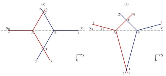
Figure 1.
(a) Geometric configuration of beams for coupled devices, version Double (axes XI and XII are opposite), plan view. Emitters A and B are separated by a distance l = AB. (b) Beams configuration after rotation of X-axes by an angle γ.
Now, assuming the Double configuration, if the X axes of the devices are rotated by an angle γ one ADCP clockwise, the other—counterclockwise) while maintaining the vertical orientation of the devices (Figure 1b), then for the range of γ from 0° to 30° beams 2, 6 and 3, 5 will still intersect, but the depths of the intersection points will change: point C will “rise” and its depth will monotonically decrease in the interval (ctg 25°, 0.5 ctg 25°), and point D will “sink” and its depth will monotonically increase from ctg 25° to ∞.
Thus, by varying the angle γ and, hence, the positions of points C and D, it is possible to scan successively the entire depth of the water column (except for the blanking zone ~10 cm directly below the emitters, where the signal is distorted by interference). The calculation of the dependence of the depths of points C and D on the angle of rotation γ is given in Appendix A, the corresponding set of lines for different values of the distance l between the emitters is shown in Figure 2. Each line of this set is presented by two branches, for points C and D correspondingly. This nomogram, along with information about the compatibility of the system of equations (see Figure 3 below), should be considered as a basis in experiment planning.
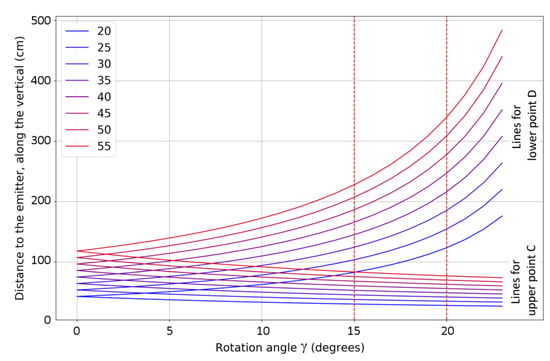
Figure 2.
Dependences of the depths of beam intersection points (h) on the angle γ and the distance between the emitters l. The legend gives the values of l in centimeters. The vertical dashed lines correspond to the values of γ used in the experiments on Lake Vendyurskoe (γ = 15°) and on Petrozavodsk Bay (γ = 20°).
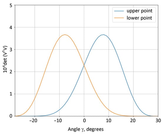
Figure 3.
Dependence of the determinant of the over determined system of equations (A7) on the rotation angle γ.
Using the expressions relating the beam velocity components to the Cartesian ones, it is possible to obtain an overdetermined system of equations for the six components of the stress tensor from the experimental data for the depths where the beam pairs intersect. This system includes six expressions for the intensity of beam velocity pulsations; the additional (seventh) equation includes the correlation of the intersecting beams’ velocities. Thus, for each fixed angle γ from the interval (0°, 30°), it is possible to calculate all six stresses for the two depths corresponding to points C and D. The derivation of the system of equations and its explicit form are given in Appendix B.
Using the standard procedure for finding an approximate solution to the overdetermined system (A7) by the least squares method, we obtain the following explicit expression for the “vector” of stresses :
Here, is a 6 × 7 matrix of coefficients; the upper index T is used to denote the transposed matrix, s = sin α0, M is the 6 × 7 matrix of coefficients with the elements determined by the angles α0 and γ, Bj is presented by six intensities of the beams velocities and velocity correlations of intersecting beans (see Appendix B).
The stress errors were calculated using the method presented in [12,13]. Under the standard assumptions (no correlations of beam components, Gaussian character of pulsations), the corresponding formulas take the form
Here, σi is the standard deviation for the component i of the vector R, n2 is the number of measurements used in ensemble averaging. Following the turnover time estimation procedure presented in [11], we chose the value 150 for the parameter n2; it corresponds to one-hour averaging. In most cases, however, the calculated stress values became “saturated” even with an averaging period of 30 min.
In connection with error estimates, it should also be emphasized that the system of equations (A7) is overdetermined, and its solutions (2) are only approximate, obtained by the least squares method. The adequacy and accuracy of such solutions, as emphasized in [9], significantly depends on the value of the determinant D of the VTV matrix, which, in turn, depends not only on the device parameter α0, but also on the angle γ, which is determined by the experiment details. The calculated dependence of D on γ is shown in Figure 3.
The value of the determinant for the upper beam intersection point depends on γ non-monotonically: in the 0–8° range it almost doubles compared to the initial (at γ = 0) value, then decreases to 0 at γ = 30°.
At the lower beam intersection point, the determinant D takes on significantly smaller values (for example, by a factor of 6 at γ = 8°) as compared to the upper point and decreases monotonically over the entire range of γ values. Accordingly, the accuracy of determining stresses at the lower intersection point will be much poorer. A significant decrease in D at both depths when approaching the threshold value γ = 30° is explained by a decrease in the angular spacing of the beams.
Thus, the value of D (and, accordingly, the accuracy of stress estimates) significantly depends on the value of the parameter γ. The proper choice of γ allows one to significantly optimize the solution and, in this regard, is an essential part of the experiment design and planning.
Another thing to remember is that the quality of the stress calculation depends significantly on the fulfillment of the horizontal homogeneity assumption, which, in turn, depends on the configuration and area of the beams’ spread at each given depth (see this spread illustrated in Figure 4). The area of beam spread increases (roughly linearly) with depth, making calculations for the lower intersection point again more problematic.
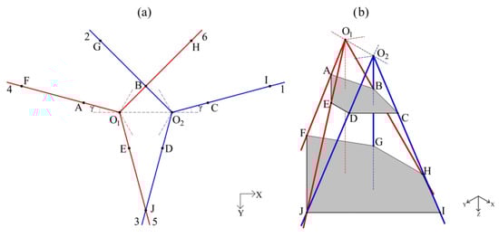
Figure 4.
(a) Beam configuration for γ ≠ 0, plan view. Points O1 and O2 correspond to the emitter locations. (b) Beam spread areas for the two depths where pairs of beams intersect. Capital Latin letters are used to designate those points at different depths where measurements of the beam velocity components were taken.
Both of these problems associated with the accuracy of stress calculations can be eliminated if the problem is limited to finding not all six components of the stress tensor, but a certain limited set of them. Stresses in the plane of beams 2 and 6 act as such a set for the upper depth, and in the plane of beams 3 and 5—for the lower depth. In each of these planes, stresses are represented by pulsation intensities along perpendicular axes (one of which can be chosen as an axis collinear with the line O1O2) and the corresponding shear stress (off-diagonal component). In turn, in each of these two planes the beam correlations, e.g., for the plane of beams 2 and 6, are available directly from observational data. On the other hand, each of these correlations can be expressed in terms of three unknown stresses. This yields a closed system of three equations for three unknowns. It should be also stressed that the horizontal homogeneity assumption is not applied in deriving this system: all the three mentioned beam correlations belong to the same point (point B for the upper and point J for the lower depth).
The above approach enables, in particular, a rigorous calculation of the pulsation intensity for both depths. The corresponding explicit expressions (which may be also derived from the explicit representation of the matrix M) for the upper and the lower depths (points B and J) are
Finally, it should be noted that for each acceptable angle γ, a stress matrix can be calculated for two specific depths. By varying the value of γ, it is possible to carry out stress profiling depthwise. As this paper focuses on testing the method, we present the results only for one fixed value of the angle γ.
We tested the method by staging two field experiments on lakes of North-Western Russia. The first experiment was conducted on Lake Vendyurskoe (62°10′ N, 33°20′ E) on 16–18 November 2021, during pre-winter open-water period. The second experiment was carried out on ice-covered Petrozavodsk Bay of Lake Onega (61°46′ N, 34°25′ E) on 14–18 April 2022.
Lake Vendyurskoe is a small shallow lake; its average and maximal depths are 5.3 and 13.4 m, respectively. For more information about this lake, including bathymetry, see [11]. During our measurements, intensive surface cooling and wind mixing were observed, so the water column was uniform in temperature, which ranged within 2.30–2.33 °C in the central deep-water part of the lake. Weak stratification was observed only in the thin 10-cm near bottom water layer, because the dynamics of this layer was also significantly affected by the heat transfer from bottom sediments. During the autumn overturn and pre-winter periods, mixing processes in Lake Vendyurskoe are very intensive throughout the water column, including the bottom water layer, and are not limited to molecular heat conduction. The mechanisms of mixing and heat transfer at the water-sediments interface have not been fully studied and still have some challenging aspects. To identify and describe these mixing mechanisms quantitatively, data on turbulence parameters (primarily turbulent stresses) are needed. Our experiment, which included scanning of the 1.85 m bottom layer, was aimed precisely at obtaining such data.
Two ADCPs (Nortek Aquadopp HR Current Profiler 2 MHz Norway) were fixed on a rigid wood panel at a distance of 43 cm from each other (distance l between emitters). The panel was fixed in the water column by bracing between the buoy and the bottom platform. The bottom platform was a triangle of metal plates, the corners of which were connected by hard rope to the central cable to which the buoy was attached (Figure 5a).
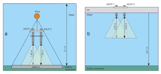
Figure 5.
Sketches of experiment designs with coupled ADCPs. (a) 16–18 November 2021, Lake Vendyurskoe. (b) 14–18 April 2022, Petrozavodsk Bay of Lake Onega.
The depth at the station was 6.1 m, and the distance from the emitters to the bottom was h = 1.85 m. Both ADCPs were operated in downlooking mode. The beam velocity components were measured in 74 cells, the discreteness Δz along the vertical (cell thickness) was 25 mm.
It has been noted above that the choice of the angle γ of rotation of each ADCP relative to differently directed X axes plays a key role in experiment planning: it is the value of γ that determines the depths at which pairs of beams intersect and, accordingly, turbulent stresses can be calculated. In our experiment, the near-bottom area was of particular interest. In this case, the lower beams’ intersection point must be chosen in such a way that the results are not distorted by the reflection from the bottom (sidelobe reflection). The critical distance from the bottom at which distortion is significant is usually determined by the formula [14]. For ADCPs with three beams, when α0 = 25°, the depth range contaminated by sidelobe relection constitutes over 9% of the scanned area; this percentage may be sufficiently enhanced by tilt variability [14]. Taking all these issues into account, we used the value 15° for the angle γ. The beam intersection points were calculated using Equations (A3) and (A4); they occurred at depths of 35 and 140 cm from the bottom.
Measurements with both ADCPs were carried out in the burst mode; burst interval was 24 s with 16 samples per burst and 2 Hz sampling frequency. Each device took measurements for 8 s, and then turned off for 16 s. The start times of the two ADCPs had a lag of 12 s, so the velocities were measured by the devices alternately and there was no superposition of the acoustic signals. Taking into account the typical interval (10−8–10−6) W/kg for the kinetic energy dissipation rate ε for shear-induced convection during open water period [15], the range of the Kolmogorov time scale td = (ν/ε can be estimated as (1–10) s. So, the expected value of td exceeded the time interval between pings (0.5 s) by up to an order of magnitude, and the active burst interval (8 s) was close to td. In view of this fact, we used the procedure of preliminarily averaging the signal within each burst (16 samples) in order to reduce the instrumental errors. The second step for calculating the mean values of the parameters includes the averaging over 1-h interval (150 samples).
The second experiment was carried out on 14–18 April 2022 in Petrozavodsk Bay of Lake Onega during the development of radiatively driven convection caused by inhomogeneous heating of the water column under the ice. Petrozavodsk Bay is located in the western part of Lake Onega. The length and width of Petrozavodsk Bay are 14 and 5 km, respectively, with a mean depth of 15 m and maximal depth of 30 m. The Shuya River flows at the end of the bay with a mean annual discharge of 96 m3/s (300 m3/s at the peak of the spring flood) [16]. More information about Petrozavodsk Bay, including bathymetry, is given in [16]. The experiment was designed to check the estimates of turbulent stresses obtained in convectively mixed layer (CML) of ice-covered lakes previously [16,17,18], as well as to supplement them by comparing the results for two different depths within CML.
Here, the same operational parameters were used as in the first experiment, but the ADCPs rotation angle γ was 20°, and the number of cells at 2.93 m scanning depth was 117. The discreteness Δz along the vertical (cell thickness) was also 25 mm. In this case, the beams intersected at depths located at distances of 58 cm and 265 cm from the lower ice surface (cells 19 and 101). Each ADCPs were installed in the hole in such a way that the emitters were directly at the lower surface of the ice (Figure 5b).
The first step in processing both sets of data was to calculate the mean velocity components. In doing so, Equations (A5) and (A6), which connect the beam velocity components with the Cartesian ones in the XYZ system, were taken into account. The calculations were carried out independently according to the data of each ADCP, which enables direct verification of the basic assumption of horizontal uniformity.
3. Results
The estimates of the mean velocity components are shown in Figure 6 and Figure 7 for Lake Vendyurskoe and Petrozavodsk Bay. In both cases, the calculations were carried out for two depths corresponding to the upper and the lower beam intersection points.
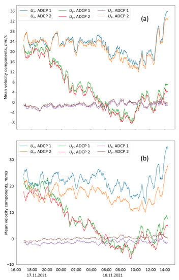
Figure 6.
The dynamics of Cartesian components of mean velocity in the bottom layer of Lake Vendyurskoe: (a) the upper beam intersection point, 140 cm above the bottom, (b) the lower beam intersection point, 35 cm above the bottom.
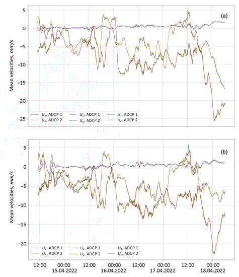
Figure 7.
The dynamics of Cartesian components of mean velocity in the under-ice layer on upper (a) and lower (b) beam intersection points. Petrozavodsk Bay of Lake Onega.
For the Petrozavodsk Bay data series, the mean velocities calculated independently from the data of each ADCP demonstrate very similar dynamics. The corresponding curves, which describe the dependence of velocity components on time, almost coincide for both depths of beam intersection; sets of curves for the upper beam intersection point of the two ADCP are presented in Figure 7. For the upper and lower beam intersection points, the correlation coefficients for independently calculated x, y and z components of mean velocity were very high (Table 1). At both depths, the assumption of horizontal homogeneity can thus be considered justified.

Table 1.
The correlation coefficients for components of mean velocity calculated independently from the data of each ADCPs.
For the upper intersection point in Lake Vendyurskoe this assumption also appears valid (Figure 6a); the values of the correlation coefficients there are quite high (Table 1) for all three velocity components. At the same time, at the lower intersection point, located 35 cm above the bottom, the discrepancies between the values of the velocity components calculated for different ADCPs were very significant (Figure 6b), significantly exceeding the measurement errors. Such discrepancies can be considered as an analogue of error velocity in experiments with a single ADCP, and, accordingly, they act as direct indicators that the horizontal homogeneity assumption does not hold.
The calculation of all six components of the stress matrix for the upper beam intersection point in Lake Vendyurskoe, where the basic assumption of horizontal homogeneity was fulfilled, was carried out by using Equation (2). The results for the diagonal components of the matrix (pulsation intensities) are presented in Figure 8. For all these three components, in contrast to the three off-diagonal ones (shear stresses), the condition of positive definiteness is satisfied almost everywhere. A more general condition for the positive definiteness of the stress matrix is also satisfied, which corroborates the physical consistency of the results. The intensitiy of pulsations along axis X was also calculated by using the exact Equation (4) instead of Equation (2). The results of both calculations were practically the same, as Figure 8 illustrates.
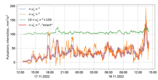
Figure 8.
Intensities of turbulent pulsations (components 11, 22 and 33 of the stress matrix) in the upper beam intersection point 140 cm above the bottom. The thick line represents the results of alternative calculations of the pulsation intensity <ux′2> performed using the exact Equation (4). Lake Vendyurskoe data.
As to the specific physical features of the results, it is worth noting the high degree of pulsation anisotropy; the intensity of pulsations along any of the horizontal axes was approximately three times higher than the intensities along the vertical.
For data from Lake Vendyurskoe the assumption of horizontal homogeneity was not entirely acceptable at the lower beam intersection point, so the calculation of all six stresses at this depth using the method described in Appendix B was not done. However, as shown above, some stress calculations can be carried out even if this strong assumption is not applicable. In particular, for both beam intersection points it is possible to calculate the pulsation intensities using Equations (4) and (5). The results of this alternative calculation of the intensities of horizontal components in the lower beam intersection point are shown in Figure 9. The shaded area along the curve represents the significance intervals calculated using Equation (3) for 95% confidence level.
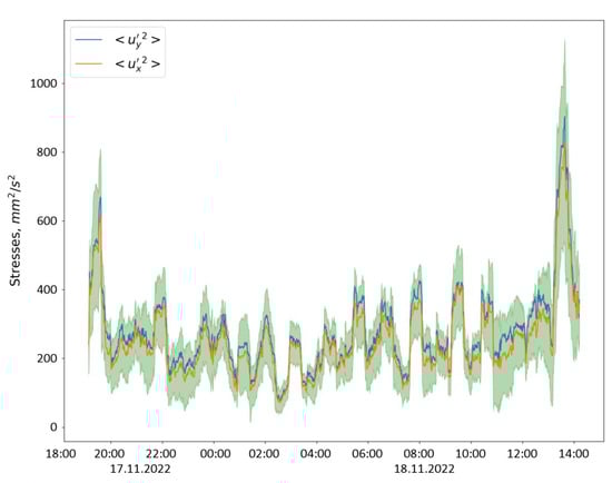
Figure 9.
Intensity of horizontal velocity component pulsations (components 11, 22 of the stress matrix) in the lower beam intersection point located 35 cm above the bottom. The shaded area represents the significance interval for the pulsations Lake Vendyurskoe data.
Some aspects of these results should be highlighted. Firstly, the intensity of horizontal pulsations at the lower beam intersection point is significantly (4–5-fold) higher than the corresponding values for the upper point, which indicates a significant hydrodynamic activity in a thin (about 35 cm) layer near the bottom. Secondly, pulsations in the horizontal plane at the lower intersection point become almost isotropic (). Finally, a noteworthy fact is the periodicity of the intensities, represented by relaxation oscillations with a period close to one hour. We regard these specific physical features as a challenge for future studies.
Calculations of all components of the stress matrix in the upper beam intersection point of the convectively mixed layer in Petrozavodsk Bay were carried out using the general Equation (2). The results are shown in Figure 10; their physical validity is confirmed again by the fact of positive definiteness of the stress matrix (only a few percent of cases do not meet this requirement).
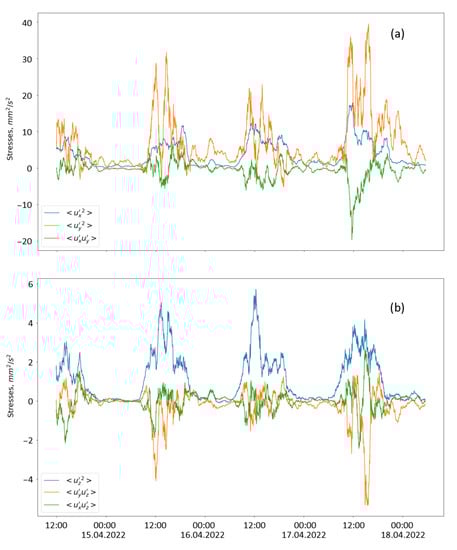
Figure 10.
Stress matrix components in the horizontal (a) and vertical (b) planes. Petrozavodsk Bay data. Distance from the lower ice surface is 58 cm.
For the lower beam intersection point, the error in the calculation of vertical fluctuations turned out to be quite significant; it was close to the value of the intensities themselves. In this regard, quantitative comparison was possible only for horizontal pulsations at different depths; they are shown in Figure 11. It is noteworthy that the variation of these pulsations with depth was considerable: the intensities of pulsations grew about four-fold compared to the distance from the lower ice surface increased from 58 to 265 cm.
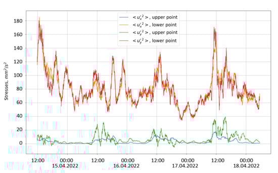
Figure 11.
Intensities of horizontal velocity component pulsations in the convectively mixed layer in the upper and lower beam intersection points at distances of 58 and 265 cm from the lower ice surface.
4. Discussion
The paper proposes a variant of the geometric configuration of two ADCPs to enable an approximate (based on the solution of an over determined system of equations) calculation of all six turbulent stresses. The main feature of this configuration is the presence of intersection points of two pairs of beams, so that this configuration can be considered as a hybrid of Aqoustic Doppler Velocimeter, where three beams intersect at one point, and a conventional profiler, which allows scanning parameters in a certain layer. Thus, this ADCP configuration provides some features that are only available when using ADV. In this method, the key aspect that allows all six stresses to be calculated is the intersection of the beams.
By manipulating the angle γ of ADCPs’ rotation in the horizontal plane (and, hence, the difference between their heading angles) we can vary the depths for which the stress calculation is performed. The accuracy of such a calculation essentially depends on the value of γ; optimal results are achieved only in the range of small angles: . The choice of the second parameter of the geometric configuration, the distance between ADCP emitters, is also subject to very significant restrictions, mainly related to the assumption of horizontal homogeneity. The spacing of ADCP emitters and, accordingly, the size of the horizontal area (beam spread) in which beam velocity components are measured have a noticeable effect on the accuracy of calculations, especially at the lower beam intersection point.
It should be noted, however, that for each of the depths where the beams intersect, three turbulent stresses on the plane of the intersection can be calculated strictly, without invoking the hypothesis of horizontal homogeneity. In particular, such calculation can be carried out for the intensity of pulsations along the axis collinear with the line connecting the ADCP emitters. In this study, such calculations were carried out for the bottom layers of a shallow lake during pre-winter period and for two depths of a convectively mixed layer in an ice-covered lake.
A general conclusion following from the calculation results is that the proposed method has a certain potential, if not for obtaining a depthwise stress profile, then at least for comparing the pulsation intensities at different depths.
Yet, there is reason to remain optimistic about the problem of water column profiling. It is associated with a possibility of automatic variation of the angle γ during the experiment. Such variation may be discrete or smooth. In the latter case, the time scale of γ variations must be consistent with the time scales of dominant physical processes (eddy turnover time, period of internal waves, etc.) within the investigated water body. Such experiments with varying γ are planned for the future.
Finally, it should be noted that the described method can also be used for other ADCP versions, e.g., four-beam (Janus) devices.
Moreover, such devices are preferable; their advantage is that nine equations can be compiled for six unknown stresses for the depths where the beams intersect. This enhances the solution accuracy of the over determined system. In addition, a smaller standard value of the slant angle of the beams (20° versus 25° in three-beam instruments) reduces the risks of the horizontal homogeneity assumption failure.
Author Contributions
Conceptualization, S.B.; methodology, S.B. and A.M.; software, S.B. and I.M.; validation, S.B.; formal analysis, S.B. and I.M.; investigation, R.Z., G.Z., N.P. and A.M.; resources, S.B. and G.Z.; data curation, S.B.; writing—original draft preparation, S.B., I.M. and G.Z.; writing—review and editing, S.B., I.M. and G.Z.; visualization, S.B., I.M. and G.Z.; supervision, S.B.; project administration, G.Z.; funding acquisition, G.Z. All authors have read and agreed to the published version of the manuscript.
Funding
The study was funded by Russian Science Foundation grant #21-17-00262 “Mixing in boreal lakes: mechanisms and its efficiency”.
Data Availability Statement
The data is available at https://drive.google.com/drive/folders/1feT42NOtNSmiKg_FGtqwHLKDii8knTeI (accessed on 18 November 2022).
Conflicts of Interest
The authors declare no conflict of interest.
Appendix A
Calculation of the depths of the points C and D where the beams intersect.
Considering the beam configuration shown in Figure 1b, we denote the unit vectors of the beams and by and , the lengths of segments AC and BC by b, and the distance AB between the emitters by l. Then, from the triangle ABC it follows that
Correspondingly:
Further, from (A1) and (A2) it follows that
As a result, the following expressions are obtained for the length b = AC:
And, finally, for the depth h1 of the point C:
After doing the same calculations for the triangle ABD, a similar expression is derived for the depth h2 of the point D:
Appendix B
Derivation of a matrix relating stress tensor components to beam velocity variances.
The beams are numbered as shown in Figure 1b; the XYZ Cartesian system is introduced in such a way that the X axis runs along the line AB connecting the centers of the devices’ emitters.
Using the direction cosines for the unit vectors that determine the directions of the beams, the beam velocities can be expressed in terms of the Cartesian velocity components:
At a depth corresponding to the beam intersection point C, the intensities of pulsations of all six beam velocities can be calculated directly from the experimental data, as well as the correlation for the intersecting beams 2 and 6. It is convenient to represent these quantities as components of a 7-dimensional vector:
In turn, by using (A5) and (A6), each component of this vector can be represented as a linear combination of the six unknown turbulent stresses. Introducing the 6-dimensional vector
The relations connecting the components of the “vectors” Bi and Ri, can be written in a compact form (summation is assumed over repeated indices):
Here, s = sin α0, M is the 6 × 7 matrix of coefficients with its elements determined by the design angle α0, as well as the angle of rotation γ:
The system of equations for the point D is derived in a similar way, while should be used as the seventh component of the vector Bi. The explicit expression for the matrix M in this case is:
References
- Nystrom, E.A.; Rehmann, C.R.; Oberg, K.A. Evaluation of mean velocity and turbulence measurements with ADCPs. J. Hydraul. Eng. 2007, 133, 1310–1318. [Google Scholar] [CrossRef]
- Gargett, A.; Wells, J. Langmuir turbulence in shallow water. Part 1. Observations. J. Fluid Mech. 2007, 576, 27–61. [Google Scholar] [CrossRef]
- Gilcoto, M.; Jones, E.; Fariña-Busto, L. Robust Estimations of Current Velocities with Four-Beam Broadband ADCPs. J. Atmos. Ocean. Technol. 2009, 26, 2642–2654. [Google Scholar] [CrossRef]
- Lu, Y.; Lueck, R.G. Using a broadband ADCP in a tidal channel. Part I: Mean flow and shear. J. Atmos. Ocean. Technol. 1999, 16, 1556–1567. [Google Scholar] [CrossRef]
- Wiles, P.J.; Rippeth, T.P.; Simpson, J.H.; Hendricks, P.J. A novel technique for measuring the rate of turbulent dissipation in the marine environment. Geophys. Res. Lett. 2006, 33, L21608. [Google Scholar] [CrossRef]
- Lucas, N.S.; Simpson, J.H.; Rippeth, T.P.; Old, C.P. Measuring Turbulent Dissipation Using a Tethered ADCP. J. Atmos. Ocean. Technol. 2014, 31, 1826–1837. [Google Scholar] [CrossRef]
- Lohrmann, A.; Hackett, B.; Roed, L.P. High resolution measurements of turbulence, velocity, and stress using a pulse-to-pulse coherent sonar. J. Atmos. Ocean. Technol. 1990, 7, 19–37. [Google Scholar] [CrossRef]
- Howarth, M.J.; Souza, A.J. Reynolds stress observations in continental shelf seas. Deep Sea Res. II 2005, 52, 1075–1086. [Google Scholar] [CrossRef]
- Vermeulen, B.; Hoitink, A.J.F.; Sassi, M.G. Coupled ADCPs can yield complete Reynolds stress tensor profiles in geophysical surface flows. Geophys. Res. Lett. 2011, 38, L06406. [Google Scholar] [CrossRef]
- Thiebaut, M.; Filipot, J.-F.; Maisondieu, C.; Damblans, G.; Duarte, R.; Droniou, E.; Guillou, S. Assessing the turbulent kinetic energy budget in an energetic tidal flow from measurements of coupled ADCPs. Phil. Trans. R. Soc. A 2020, 378, 20190496. [Google Scholar] [CrossRef] [PubMed]
- Bogdanov, S.R.; Zdorovennov, R.E.; Palshin, N.I.; Zdorovennova, G.E.; Terzhevik, A.Y.; Gavrilenko, G.G.; Volkov, S.Y.; Efremova, T.V.; Kuldin, N.A.; Kirillin, G.B. Deriving of Turbulent Stresses in a Convectively Mixed Layer in a Shallow Lake Under Ice by Coupling Two ADCPs. Fundam. Prikl. Gidrofiz. 2021, 14, 17–28. [Google Scholar] [CrossRef]
- Stacey, M.T.; Monismith, S.G.; Burau, J.R. Measurements of Reynolds stress profiles in unstratified tidal flow. J. Geophys. Res. 1999, 104, 10933–10949. [Google Scholar] [CrossRef]
- Williams, E.; Simpson, J.H. Uncertainties in Estimates of Reynolds Stress and TKE Production Rate Using the ADCP Variance Method. J. Atmos. Ocean. Technol. 2004, 21, 347–357. [Google Scholar] [CrossRef]
- Lentz, S.J.; Kirincich, A.; Plueddemann, A.J. A Note on the Depth of Sidelobe Contamination in Acoustic Doppler Current Profiles J. Atmos. Ocean. Technol. 2022, 39, 31–35. [Google Scholar] [CrossRef]
- Bouffard, D.; Wüest, A. Convection in lakes. Annu. Rev. Fluid Mech. 2019, 51, 189–215. [Google Scholar] [CrossRef]
- Bogdanov, S.; Zdorovennova, G.; Volkov, S.; Zdorovennov, R.; Palshin, N.; Efremova, T.; Terzhevik, A.; Bouffard, D. Structure and dynamics of convective mixing in Lake Onego under ice-covered conditions. Inland Waters 2019, 9, 177–192. [Google Scholar] [CrossRef]
- Volkov, S.; Bogdanov, S.; Zdorovennov, R.; Zdorovennova, G.; Terzhevik, A.; Palshin, N.; Bouffard, D.; Kirillin, G. Fine scale structure of convective mixed layer in ice-covered lake. Environ. Fluid Mech. 2019, 19, 751–764. [Google Scholar] [CrossRef]
- Bogdanov, S.; Zdorovennov, R.; Palshin, N.; Zdorovennova, G. Deriving Six Components of Reynolds Stress Tensor from Single-ADCP Data. Water 2021, 13, 2389. [Google Scholar] [CrossRef]


Disclaimer/Publisher’s Note: The statements, opinions and data contained in all publications are solely those of the individual author(s) and contributor(s) and not of MDPI and/or the editor(s). MDPI and/or the editor(s) disclaim responsibility for any injury to people or property resulting from any ideas, methods, instructions or products referred to in the content. |
© 2022 by the authors. Licensee MDPI, Basel, Switzerland. This article is an open access article distributed under the terms and conditions of the Creative Commons Attribution (CC BY) license (https://creativecommons.org/licenses/by/4.0/).