Using Self-Organizing Map and Multivariate Statistical Methods for Groundwater Quality Assessment in the Urban Area of Linyi City, China

Abstract

Groundwater holds an important role in the water supply in Linyi city, China. Investigating the hydrochemical characteristics of groundwater, and revealing the factors governing groundwater geochemistry, is a primary step for ensuring the safe and rational exploitation of groundwater resources. This study used a self-organizing map (SOM) and multivariate statistical methods to assess groundwater quality in the urban area of Linyi city. Based on the hydrochemical dataset consisting of nine parameters (i.e., pH, ${\mathrm{C}\mathrm{a}}^{2+}$, ${\mathrm{M}\mathrm{g}}^{2+}$, ${\mathrm{N}\mathrm{a}}^{+}$, ${\mathrm{K}}^{+}$, ${\mathrm{H}\mathrm{C}{\mathrm{O}}_3}^{-}$, ${\mathrm{C}\mathrm{l}}^{-}$, ${{\mathrm{S}\mathrm{O}}_4}^{2-}$, and ${{\mathrm{N}\mathrm{O}}_3}^{-}$) from 89 groundwater samples, the SOM was first applied to obtain the weight vectors of the output nodes. Hierarchical cluster analysis (HCA) was used for organizing the nodes into four clusters. The node cluster indices were then remapped to the groundwater samples according to the winner node for each sample. The hydrochemical characteristics and factors controlling the groundwater geochemistry of the four clusters were analyzed using principal component analysis (PCA) and graphical methods including Piper and Gibbs diagrams, as well as binary plots of the major ions in groundwater. Results indicated that groundwater geochemistry in this area is primarily governed by water–rock interactions, such as the dissolution of halite, calcite, and gypsum, along with the influence of municipal sewage and the degradation of organic matter. This study demonstrates that the integration of an SOM and multivariate statistical methods improves the understanding of groundwater geochemistry and hydrochemical evolution in complex groundwater flow systems impacted by utilization.

1. Introduction

Groundwater quality has received increasing attention worldwide, particularly in urban areas where groundwater resources have been significantly overexploited and polluted due to population growth and rapid industrial advancement [1,2,3,4]. The primary work in efficiently safeguarding groundwater resources is to understand the hydrochemical characteristics and the underlying factors governing groundwater geochemistry [5,6,7]. The work is complicated, because the hydrochemical data are generally complex. The hydrochemical composition of groundwater usually has multiple physical and chemical parameters, the values of which are influenced by natural processes (e.g., the dissolution and precipitation of different minerals) [8,9] and anthropogenic activities (e.g., agricultural, industrial, and domestic pollutions) [10,11,12]. These values exhibit a broad spectrum of variability, revealing intricate, non-linear relationships between explanatory and response variables, often intermingled with noise, redundancy, and outliers [13]. Explaining the variation in the complex hydrochemical data and revealing the factors behind the data is still an open research challenge.

Utilizing machine learning and artificial intelligence methods for groundwater quality analysis has gained significant popularity in recent years [14,15,16]. These methods possess a natural advantage in their ability to abstract high-dimensional data into concise features and unveil the nonlinear relationships among complex variables. Approaches such as artificial neural networks (ANNs) [17,18], adaptive neuro-fuzzy inference systems [19,20], support vector machines (SVMs) [21], and ensemble machine learning [22] have been effectively used for evaluating and predicting water quality. Among these methods, the application of self-organizing maps (SOMs) and multivariate statistical methods (e.g., hierarchical cluster analysis (HCA) and principal component analysis (PCA)), in conjunction with hydrochemical analyses, have shown their great potential to promote the understanding of the formation and evolution of groundwater chemistry [23,24,25,26,27]. As an unsupervised machine learning approach, SOMs exhibit remarkable visualization capabilities, including the component planes that use the weight vectors (also known as reference or codebook vectors) of the output nodes to give an informative representation of the input data. By comparing patterns in identical positions among the component planes, the relationships among the hydrogeochemical parameters can be identified [28,29]. The HCA serves as an effective tool to divide groundwater samples into different clusters. Samples with similar hydrochemical compositions are clustered together, while samples with distinct hydrochemical compositions are grouped in different clusters. These clusters may potentially represent distinct hydrochemical facies or water types, governing by specific controlling factors [5,7,30]. The PCA method seeks to reduce multidimensional hydrochemical data into lower dimensions, while endeavoring to retain the inherent characteristics of the original data to the maximum extent. This makes it possible to visualize the high-dimensional geochemical data in a two-dimensional map, in which the patterns embedded in the high-dimensional space may be easily captured [31,32]. Accompanying the HCA method, it has been found that PCA plots can generally distinguish the clustered data, producing a clear interpretation of the geochemical evolution [5].

In this study, an SOM, multivariate statistical methods, and graphical methods were utilized to scrutinize the hydrochemical characteristics of groundwater samples in the urban area of Linyi city, China. Linyi is an important commercial and industrial city in Shandong Province, China, and groundwater holds an important role in water supply due to the lack of surface water in this area. Previous studies have reported various groundwater issues, including overexploitation [33], groundwater pollution, and the lack of a functional groundwater monitoring network in this area [34]. However, there exists limited knowledge about the hydrochemical characteristics and the governing factors of groundwater geochemistry in this area. Therefore, the aims of this study are to: (1) classify the groundwater samples by using an SOM and multivariate statistical methods; (2) investigate the hydrochemical characteristics of the groundwater samples from different clusters, and (3) reveal the controlling factors governing groundwater geochemistry. Our achievements are expected to promote a better understanding of groundwater quality and to provide important references for the rational development and protection of groundwater in Linyi city.

2. Study Area

Linyi city is situated in the southeastern part of Shandong Province, China, characterized by elevated terrain to the north and lower elevation towards the south and west (Figure 1). This area is subjected to a semi-humid temperate continental monsoon climate, with cold-dry winters and hot-rainy summers. The annual average temperature is 14 °C, accompanied by an annual average precipitation of 813 mm [35]. Most of the precipitation occurs between June and September, accounting for about 73% of the total annual precipitation [36]. The mean annual evaporation is 1687 mm and approximately 50% of the evaporation occurs from March to June. The main rivers across the study area are Yi River and its three tributaries, Fang River, Su River, and Liuqing River (Figure 1). Controlled by the topography, the rivers regionally flow from the north to south.

According to the previous study [37], aquifer systems can be classified into four different types: (1) pore water-filling aquifer, (2) karst fissure water-filling aquifer, (3) clastic fissure water-filling aquifer, and (4) bedrock fissure water-filling aquifer (Figure 2). The pore water-filling aquifer mainly contains loose Quaternary sediments, and is widely distributed in the study area. The karst fissure water-filling aquifer, formed by limestone, is mainly distributed in the west of the study area beneath the pore water filling aquifer. The clastic fissure water-filling aquifer is mainly distributed on the edges of igneous rock located in the eastern and northern areas. This aquifer is mainly formed by shale and sandstone. The bedrock fissure water-filling aquifer mainly occurs in the east, with very small proportions and weak fissure development. This aquifer is mainly formed by andesite, basalt, and other magmatic rocks.

Figure 2 suggests the highly probable presence of connections between the four aquifers. The pore water-filling aquifer receives recharge from atmospheric precipitation and underground runoff originating from adjacent aquifers upstream. In certain localized areas, there is also a contribution from top support recharge provided by the karst fissure water-filling aquifer. Furthermore, under specific conditions, such as extreme water extraction from the pore water-filling aquifer, faults can act as conduits for transporting groundwater from the classic fissure and bedrock fissure water-filling aquifers.

3. Materials and Methodology

3.1. Sample Collection and Analytical Methods

In July 2013, a total of 92 groundwater samples from private, municipal and observation wells were collected in the urban area of Linyi city. These wells were typically purged by pumping for at least 30 min to remove the water in the casing column. Groundwater samples were then collected using two 50-mL sterilized HDPE bottles after being filtered using 0.45 μm membrane filters. The first bottle was acidified to pH ≤ 2 using ultra-pure HNO₃ for analysis of cations and the second bottle was not acidified for the analysis of anions. The two bottles of each sample were sealed with watertight caps and immediately stored in a cool box with ice packs. All samples were transported to the laboratory within 24 h and stored in a refrigerator (the temperature was about 4 °C) until measurements were performed.

Temperature, pH, and total dissolved solids (TDS) were measured in situ by a portable multi-meter device (WTW multi 3400i, Weilheim, Bavaria, Germany). Concentrations of ${\mathrm{H}\mathrm{C}{\mathrm{O}}_3}^{-}$ were measured within 24 h using an acid-based titration method. Concentrations of the major anions (${\mathrm{C}\mathrm{l}}^{-}$, ${{\mathrm{S}\mathrm{O}}_4}^{2-}$, and ${{\mathrm{N}\mathrm{O}}_3}^{-}$) were determined by ion chromatograph (Dionex ICS-2500, Sunnyvale, CA, USA) with detection limits of 0.04 mg/L. Concentrations of the major cations (${\mathrm{N}\mathrm{a}}^{+}$, ${\mathrm{K}}^{+}$, ${\mathrm{C}\mathrm{a}}^{2+}$, and ${\mathrm{M}\mathrm{g}}^{2+}$) were analyzed by inductively coupled plasma-optical emission spectrometry (ICP-OES) (Thermo Fisher ICAP-6300, Waltham, MA, USA) with detection limits of 0.2 mg/L. Those measurements were all conducted in the Testing Center of Shandong Bureau of China Metallurgical Geology Administration.

3.2. Data Screening and Pre-Processing

The initial dataset consisted of 89 groundwater samples with 11 physical and chemical parameters, i.e., temperature, pH, TDS, ${\mathrm{C}\mathrm{a}}^{2+}$, ${\mathrm{M}\mathrm{g}}^{2+}$, ${\mathrm{N}\mathrm{a}}^{+}$, ${\mathrm{K}}^{+}$, ${\mathrm{H}\mathrm{C}{\mathrm{O}}_3}^{-}$, ${\mathrm{C}\mathrm{l}}^{-}$, ${{\mathrm{S}\mathrm{O}}_4}^{2-}$, and ${{\mathrm{N}\mathrm{O}}_3}^{-}$. To improve the data quality prior to the statistical analyses, the charge balance error (CBE) of each sample was calculated by using the concentrations of the four major cations and four major anions. Following previous studies [12,38], three groundwater samples with CBEs greater than 10% were excluded from further analysis. Among the 11 selected parameters, temperature was excluded from further analysis since it primarily represents a physical characteristic of groundwater, whereas the current study places emphasis on groundwater geochemistry. TDS was excluded due to its derivability from other parameters [39]. The final dataset utilized for the SOM and multivariate statistical analyses comprises 801 chemical measurements, structured within a data matrix containing 89 rows and 9 columns. These dimensions correspond, respectively, to the 89 groundwater samples and the 9 geochemical parameters attributed to each individual sample.

Given the assumption of normality inherent in multivariate statistical analysis [40], the nature-based log-transformation was applied to the nine parameters to improve the normality of the distributions. The transformed data were then standardized by using z-score normalization, i.e., subtracting the feature mean and dividing by the feature standard deviation, to remove the impacts of the parameter units on the statistical analysis. This allows all the parameters to move in approximately the same ranges and ensures that parameters with extremely different standard deviations are weighted equally in the statistical analysis [5].

3.3. Self-Organizing Map

The SOM is a distinctive variant of artificial neural networks, which aims at projecting high-dimensional input data onto a low-dimensional (usually two-dimensional) map while preserving the topological properties of the input data [41]. Given that the SOM technique has been thoroughly described in the literature [29,42,43], we only describe how it was used in this study. The SOM was first applied to the standardized geochemical data to obtain the weight factors with the commonly used hexagonal array. The number of nodes was determined by following the rule of thumb, $m=5\sqrt{n}$ [29], where m denotes the number of the SOM nodes and n represents the number of input data sources, i.e., n = 89 in this study. The ratio between the number of rows and columns in the SOM map was determined using the square root of the ratio between the two largest eigenvalues extracted from the standardized geochemical data [43]. Weight vectors were initialized by using the PCA method, that is, the weights were initialized by spanning the first two principal components to make the training process converge faster. The SOM training was carried out with 5000 iterations, which was determined by trial-and-error experiments, and by using Euclidean distance measure with Gaussian neighborhood function. The starting learning rate and neighborhood radius were set to be 0.05 and 1.0 by default in the algorithm, respectively. These two parameters both decreased as the iterations progressed by using asymptotic decay. Taking the learning rate as an example, $\alpha \left(t\right)={\alpha }_0/\left(1+t/T\right)$ where $\alpha \left(t\right)$ denotes the learning rate of the t-th iteration, ${\alpha }_0$ is the starting learning rat, and T equals the total number of iterations divided by two (i.e., $\mathrm{T}=2500$ in this study). During the SOM training process, the weight vectors were iteratively updated using batch mode. This means that the SOM was trained using all the vectors in the data sequentially, rather than being randomly picked. The continuation of this training process persisted until a predefined stopping criterion was fulfilled, denoted by the stabilization of the weight vectors or the attainment of the specified number of iterations. The weight vectors obtained at the end of the training process were employed to identify the winner node, defined as the node whose weight vector was closest to the input vector.

Interpretation of the SOM results was conducted through the U-matrix and component planes. The U-matrix, signifying the unified distance matrix, is a visual representation of the SOM, illustrating the Euclidean distances between the weight vectors of adjacent nodes. The component planes illustrate the distribution of the weight vectors in each dimension onto the same geometry. Visualization of the component planes of the SOM provides a distinctive opportunity to scrutinize the distribution of individual input variables, all the while encompassing the congruity of the input records across the full spectrum of variables. The integration of all component planes within a single visualization (where parallel gradients may indicate positive correlations) further facilitates the discernment of qualitative associations amongst variables. For the SOM implementation, Python with MiniSom library (https://pypi.org/project/MiniSom/, accessed on 24 August 2023) was utilized in this study.

3.4. Multivariate Statistical and Graphical Methods

In this study, HCA was conducted with Ward’s linkage criteria and the Euclidean distance measure. The distance of the weight vectors between a pair of SOM nodes was calculated, and then Ward’s method was used to employ an analysis of variance framework to minimize the increase in the total within-cluster variance between any two potential clusters formed at each step of the clustering process [44]. This produces a tree-like diagram called dendrogram. The determination of the optimal number of clusters is guided by the phenon line, and its placement on the dendrogram dictates the number of clusters formed. Additionally, the Silhouette coefficient method was applied to help determine the optimal number of clusters. The Silhouette coefficient, ranging from −1 to 1, quantifies the quality of clustering. Higher Silhouette coefficients indicate more favorable clustering results [6].

PCA was carried out for factor extraction by reducing the nine parameters down to a few uncorrelated components. The generated components are expected to capture the underlying processes responsible for correlations among variables. Principal components with eigenvalues exceeding 1, as recommended by Kaiser [45], are permissible to be analyzed. The factors produced from the PCA represent the possible sources of the hydrochemical composition of groundwater. Additionally, the graphical methods, including Piper and Gibbs diagrams and binary plots of the geochemical concentrations, were used for facilitating the geochemical analyses. HCA and PCA were performed using SciPy package (https://scipy.org/, accessed on 24 August 2023) in Python environment. The Piper and Gibbs diagrams were drawn by using WQChartPy Package [46]. The overall methodological flow chart of this study is shown in Figure 3.

4. Results and Discussion

4.1. SOM and Statistical Results

The input data used for the SOM training consisted of the standardized concentrations of the nine parameters of the 89 groundwater samples after log-transformation. Based on the methodology described above, the total number of SOM nodes was determined as 48, distributed over eight rows and six columns. Figure 4 illustrates the nine component planes obtained after the training process. Each map represents the component values of the weight vectors for the 48 SOM nodes organized by eight rows and six columns. A comparative analysis of the component planes, presented through varying color gradients, helps to interpret the underlying data distribution and relationships. If two maps have similar activation positions, then this represents the possibility of a positive correlation between the two parameters. If the two maps have opposite activation positions, then this represents a negative correlation. Upon visual examination of the component maps in Figure 4, it is evident that ${\mathrm{N}\mathrm{a}}^{+}$, ${\mathrm{K}}^{+}$, and ${\mathrm{C}\mathrm{l}}^{-}$ share similar color gradients, indicating a positive correlation among these three parameters. This observation is mirrored in the component planes of ${\mathrm{C}\mathrm{a}}^{2+}$ and ${\mathrm{M}\mathrm{g}}^{2+}$, which also suggests that there is a positive correlation between ${\mathrm{C}\mathrm{a}}^{2+}$ and ${\mathrm{M}\mathrm{g}}^{2+}$. This is reasonable, considering ${\mathrm{C}\mathrm{a}}^{2+}$ and ${\mathrm{M}\mathrm{g}}^{2+}$ are mainly dissolved from carbonate minerals, which also produce ${\mathrm{H}\mathrm{C}{\mathrm{O}}_3}^{-}$. Moreover, given that ${\mathrm{C}\mathrm{a}}^{2+}$ and ${{\mathrm{S}\mathrm{O}}_4}^{2-}$ are partially derived from the dissolution of sulfate minerals, such as gypsum, this explains the positive relationship between ${\mathrm{C}\mathrm{a}}^{2+}$ and ${{\mathrm{S}\mathrm{O}}_4}^{2-}$. In contrast, ${{\mathrm{N}\mathrm{O}}_3}^{-}$ illustrates a weak correlation with the other parameters, suggesting a distinct source. To further validate the strength of these relationships depicted in Figure 4, Spearman’s rank correlation coefficients were calculated among the nine geochemical parameters, as shown in

Table 1. Spearman’s rank correlation coefficients among the nine geochemical parameters. Bold values indicate the highest absolute correlation coefficients for individual columns.

	pH	${\mathbf{K}}^{+}$	${\mathbf{N}\mathbf{a}}^{+}$	${\mathbf{C}\mathbf{a}}^{2+}$	${\mathbf{M}\mathbf{g}}^{2+}$	${\mathbf{C}\mathbf{l}}^{-}$	${{\mathbf{S}\mathbf{O}}_4}^{2-}$	${\mathbf{H}\mathbf{C}{\mathbf{O}}_3}^{-}$
${\mathrm{K}}^{+}$	0.09
${\mathrm{N}\mathrm{a}}^{+}$	−0.12	0.56
${\mathrm{C}\mathrm{a}}^{2+}$	−0.45	−0.07	0.32
${\mathrm{M}\mathrm{g}}^{2+}$	−0.16	0.27	0.53	0.55
${\mathrm{C}\mathrm{l}}^{-}$	−0.26	0.23	0.62	0.53	0.63
${{\mathrm{S}\mathrm{O}}_4}^{2-}$	−0.24	0.40	0.51	0.65	0.53	0.40
${\mathrm{H}\mathrm{C}{\mathrm{O}}_3}^{-}$	−0.32	−0.08	0.31	0.63	0.43	0.22	0.29
${{\mathrm{N}\mathrm{O}}_3}^{-}$	−0.09	−0.05	0.08	0.27	0.20	0.12	0.07	0.18

. The results show that the relationships between those parameters are consistent with the findings in the qualitative correlations from Figure 4 as mentioned above.

Figure 5 shows the clustering results on the weight vectors of the 48 SOM nodes. In Figure 5d, it’s evident that, although the Silhouette coefficient reaches its peak (0.21) with two clusters, the Silhouette coefficient for four clusters (0.20) is very close to that peak value. Additionally, there is a noticeable decline in the Silhouette coefficient when the number of clusters exceeds four. Therefore, that number of four clusters was selected as the optimum number in this study. As shown in Figure 5c, the phenon line drawn at the linkage distance of seven led to four clusters of the SOM nodes, denoted as clusters C1–C4. It is evident that clusters C1 and C2 exhibit the smallest inter-cluster distance, or the highest degree of similarity. This observation implies that cluster C1 shares hydrogeochemical characteristics akin with cluster C2. Similarly, clusters C3 and C4 also demonstrate analogous characteristics. The U-matrix of Figure 5b showed similar patterns. Figure 5a presents the pattern classification map illustrating the arrangement of the four clusters, wherein the labels within the nodes correspond to the sample names. Simultaneous analysis of the component SOM maps of Figure 4 and Figure 5 reveals what kind of data the respective clusters may include. For example, cluster C1 (lower right of Figure 5a) is associated with high concentrations of ${\mathrm{N}\mathrm{a}}^{+}$, ${\mathrm{K}}^{+}$, ${\mathrm{C}\mathrm{l}}^{-}$ and ${{\mathrm{N}\mathrm{O}}_3}^{-}$, which can be observed in the lower right of the respective component planes, as shown in Figure 4.

To further verify the results of the cluster analysis, clusters were plotted into biplots using principal components, as shown in Figure 6. The four clusters are distinctly demarcated from one another, despite some slight overlapping. This observation indicates that the cluster classification is reasonable in terms of effectively grouping the measurements of groundwater geochemistry. Three components with eigenvalues greater than one were extracted from the PCA, accounting for 69.42% of the total variance. The first principal component (PC1) accounts for 40.35% of the total variance, which is dominated by ${\mathrm{C}\mathrm{a}}^{2+}$ and ${\mathrm{M}\mathrm{g}}^{2+}$, whose loading values were 0.42 and 0.44, indicating that this component mainly represents the dissolution of carbonate minerals. The second principal component (PC2) accounted for 18.26% of the total variance, of which ${\mathrm{K}}^{+}$ is the most closely related parameter with loading values of 0.62, indicating that this component may reflect the impact of anthropogenic activities like agriculture activity on groundwater. This aligns with the findings from a previous study of Yong et al. [33], wherein they ascertained that agricultural practices constituted a significant share of water consumption in the exploitation of groundwater resources. The third principal component (PC3) accounts for 10.81% of the total variance, and this component was closely related to pH, whose loading value is 0.63, indicating the influence of pH on groundwater quality.

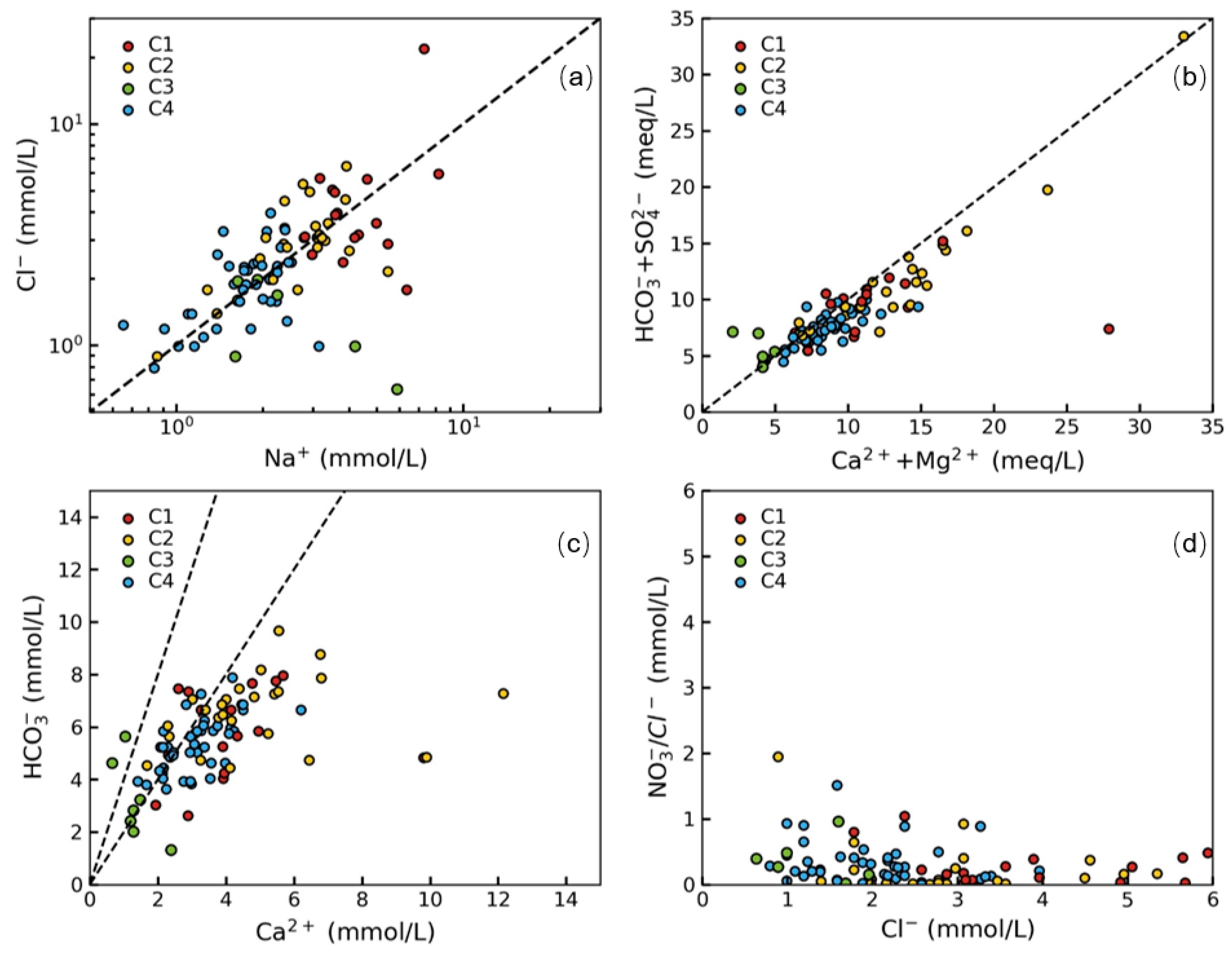
4.2. Geochemical Characteristics of the Classified Four Clusters

Table 2. The statistical characteristics of the nine parameters for the 89 samples. All units are in mg/L except for pH, which is in the standard unit.

	Maximum	Minimum	Average	Median	Standard Deviation
pH	7.96	6.82	7.35	7.28	0.26
${\mathrm{K}}^{+}$	85.31	0.20	5.14	2.27	11.66
${\mathrm{N}\mathrm{a}}^{+}$	188.41	15.00	60.95	51.80	32.32
${\mathrm{C}\mathrm{a}}^{2+}$	485.89	26.08	145.97	133.52	74.93
${\mathrm{M}\mathrm{g}}^{2+}$	104.70	9.47	32.90	30.55	16.02
${\mathrm{C}\mathrm{l}}^{-}$	777.18	22.51	98.75	82.95	85.64
${{\mathrm{S}\mathrm{O}}_4}^{2-}$	1253.90	22.05	152.91	110.10	156.96
${\mathrm{H}\mathrm{C}{\mathrm{O}}_3}^{-}$	590.48	79.96	340.57	345.06	95.42
${{\mathrm{N}\mathrm{O}}_3}^{-}$	194.44	0.89	42.41	26.30	46.86

provides an overview of the statistical characteristics encompassing the maximum, minimum, average, median, and standard deviation values of the nine parameters for all 89 groundwater samples utilized in this study. Notably, both the average and median values of pH hover around 7.3, suggesting a weak alkaline environment. Additionally, it’s worth mentioning that the average concentrations of ${\mathrm{K}}^{+}$ and ${{\mathrm{N}\mathrm{O}}_3}^{-}$ significantly exceed their respective median values, indicating a skewed distribution in the concentration values of these two parameters.

For a comprehensive grasp of the hydrochemical characteristics of the four clusters, Figure 7 presents box plots detailing the nine geochemical parameters corresponding to each cluster. Cluster C1 stands out, with a notably elevated median concentration of ${\mathrm{K}}^{+}$, ${\mathrm{N}\mathrm{a}}^{+}$, and ${\mathrm{C}\mathrm{l}}^{-}$. Meanwhile, cluster C2 exhibits a relatively low median concentration of ${\mathrm{K}}^{+}$, but counters with elevated concentrations of ${\mathrm{C}\mathrm{a}}^{2+}$, ${\mathrm{M}\mathrm{g}}^{2+}$, and ${\mathrm{H}\mathrm{C}{\mathrm{O}}_3}^{-}$. Cluster C3 exhibits excessively low concentrations of ${\mathrm{C}\mathrm{a}}^{2+}$ and ${\mathrm{H}\mathrm{C}{\mathrm{O}}_3}^{-}$ and cluster C4 is characterized by low concentrations of ${\mathrm{N}\mathrm{a}}^{+}$ and ${\mathrm{K}}^{+}$.

Figure 8 plots the Piper diagram for the 89 groundwater samples. As shown in Figure 8, water samples of cluster C1 belong to calcium and mixed types in terms of cationic characteristics. As for the anions, water samples of cluster C1 belong to bicarbonate and mixed types. Therefore, water samples of cluster C1 can be classified into Ca-HCO₃ and mixed types. Water samples of cluster C2 are distributed widely in the Piper diagram, falling into both calcium and mixed types in terms of their cationic characteristics. As for anionic characteristics, most samples of cluster C2 belong to sulphate, mixed, and bicarbonate types. Therefore, water samples of this cluster can be classified into Ca-HCO₃, Ca-SO₄ and mixed types. For water samples of cluster C3, in terms of cationic characteristics, mixed type and sodium and potassium types can be observed. In terms of anionic characteristics, sulphate, mixed, and bicarbonate types can be clearly observed. For the water samples of cluster C4, in terms of cation characteristics, most of them belong to calcium type, and a few samples belong to mixed type. In terms of anions, most water samples of this cluster belong to bicarbonate type. Figure 8 illustrates that most of the groundwater samples are Ca-HCO₃ and mixed types. The widely distributed karst fissure water-filling aquifer may explain the reason. This observation corroborates the findings of previous studies by Yong et al. [33] and Xin et al. [34], wherein they discerned that the groundwater flow in the region exhibited notable swiftness, primarily manifesting as hydrochemical bicarbonate-type water. The mixed type also highlights the complex geochemical conditions in this area.

4.3. Factors Governing Groundwater Geochemistry

While initially designed to summarize the evolution of surface water chemistry, Gibbs diagrams have proven their ability to identify the processes governing groundwater geochemistry. As depicted in Figure 9, the Gibbs diagrams have been employed to represent the hydrochemical characteristics of the four classified clusters of the 89 groundwater samples. Notably, a significant proportion of samples are situated within the rock dominance field. This strongly suggests that water–rock interactions stand as the primary process governing the chemical composition of groundwater in the study area.

The origin of ${\mathrm{N}\mathrm{a}}^{+}$ and ${\mathrm{K}}^{+}$ in groundwater can be reflected through the comparison of molar concentrations of these two parameters. As shown in Figure 10a, the molar ratios of ${\mathrm{N}\mathrm{a}}^{+}$ and ${\mathrm{C}\mathrm{l}}^{-}$ in groundwater can be reflected through the comparison of molar concentrations of these two parameters. As shown in Figure 10a, the molar ratios of ${\mathrm{N}\mathrm{a}}^{+}/{\mathrm{C}\mathrm{l}}^{-}$ of the 89 groundwater samples are generally distributed around the 1:1 line with minor fluctuations, except for samples of cluster C3. This consistent pattern signifies that Na⁺ and Cl⁻ in the groundwater of this region primarily stem from halite dissolution. The elevated Na⁺ concentration of cluster C3 is likely due to the dissolution of albite. It should be noted that because mineralogical compositions of the aquifer are unknown, rigorous proof requires follow-up studies. Figure 10b illustrates the milliequivalent concentrations of (${\mathrm{C}\mathrm{a}}^{2+}{ + \mathrm{M}\mathrm{g}}^{2+}$) against (${{\mathrm{H}\mathrm{C}\mathrm{O}}_3}^{-}+{{\mathrm{S}\mathrm{O}}_4}^{2-}$). It illustrates that the groundwater samples generally fall around the 1:1 line, suggesting that the ${\mathrm{C}\mathrm{a}}^{2+}$, ${{\mathrm{S}\mathrm{O}}_4}^{2-}$ and ${\mathrm{H}\mathrm{C}{\mathrm{O}}_3}^{-}$ levels can be largely attributed to the dissolution of gypsum and carbonate minerals. In discerning the origin of ${\mathrm{C}\mathrm{a}}^{2+}$ from the dissolution of calcite or dolomite, Figure 10c illustrates the molar concentrations of ${\mathrm{C}\mathrm{a}}^{2+}$ and ${\mathrm{H}\mathrm{C}{\mathrm{O}}_3}^{-}$, and the data fall around the 1:2 line. This observation serves as evidence for the dissolution of calcite rather than dolomite, as indicated by the molar ratio of ${\mathrm{C}\mathrm{a}}^{2+}/{\mathrm{H}\mathrm{C}{\mathrm{O}}_3}^{-}$ being 1:2 for calcite dissolution and 1:4 for dolomite dissolution. Figure 10d plots the molar ratio of ${{\mathrm{N}\mathrm{O}}_3}^{-}/{\mathrm{C}\mathrm{l}}^{-}$ versus the ${\mathrm{C}\mathrm{l}}^{-}$ concentration for the four clusters. Figure 9 elucidates the molar ratio of ${{\mathrm{N}\mathrm{O}}_3}^{-}/{\mathrm{C}\mathrm{l}}^{-}$ against ${\mathrm{C}\mathrm{l}}^{-}$ concentrations for the four clusters. Notably, samples of cluster C1 exhibit elevated ${\mathrm{C}\mathrm{l}}^{-}$ concentrations and lower ${{\mathrm{N}\mathrm{O}}_3}^{-}/{\mathrm{C}\mathrm{l}}^{-}$ ratios. This observation suggests the possible influence of municipal sewage and animal manure, as groundwater influenced by these sources typically manifests elevated ${\mathrm{C}\mathrm{l}}^{-}$ concentrations coupled with comparatively low ${{\mathrm{N}\mathrm{O}}_3}^{-}$ concentrations.

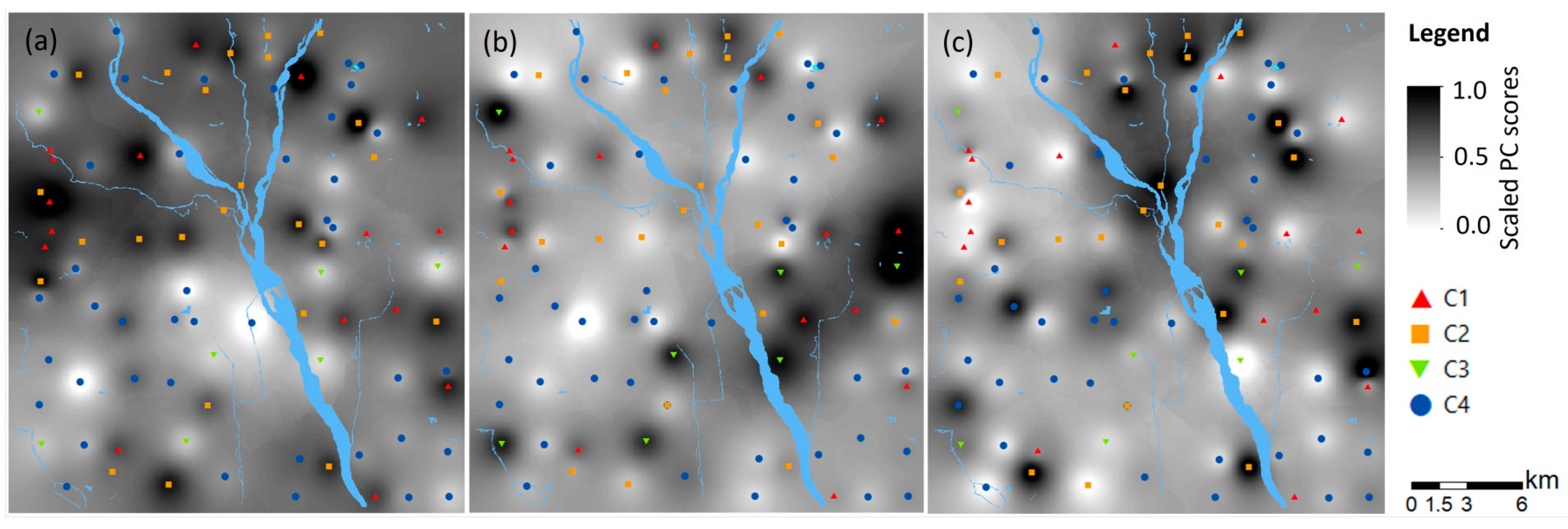
4.4. Spatial Distributions of the Four Clusters and Principal Component Scores

Figure 11 depicts the spatial distribution of the four clusters, overlaid by the spatial distributions of the first three principal component scores interpolated by the inverse distance weighted (IDW) method. To facilitate comparison, the scores for each principal component were scaled between zero and one using min-max standardization. Figure 11a illustrates that groundwater samples of clusters C1 and C2 with high PC1 scores are mainly located at the northwest of the study area, where the karst fissure water-filling aquifer occurs. As mentioned earlier, PC1 is dominated by ${\mathrm{C}\mathrm{a}}^{2+}$ and ${\mathrm{M}\mathrm{g}}^{2+}$ from the dissolution of carbonate minerals. This may explain the high PC1 scores of samples from clusters C1 and C2. Figure 11b shows that samples of cluster C3 with high PC2 scores are mainly located at the center east part of the study area. Considering PC2 is dominated by ${\mathrm{K}}^{+}$ and the municipal sewage generally contains high ${\mathrm{K}}^{+}$ concentrations [48], this implies that anthropogenic activities may have some impact in this area. Figure 11c illustrates that the samples from clusters C3 and C4 with high PC3 scores are mainly located at the center north of the study area. Considering that PC3 is dominated by $\mathrm{p}\mathrm{H}$ which is mainly controlled by dissolved CO₂, the enriched CO₂ may come from degradation of organic matter in aquifer.

In summary, the groundwater geochemistry in the northwestern region of the study area is primarily governed by calcite dissolution, whereas in the central-eastern part, anthropogenic activities exert a prominent influence. Furthermore, the prevailing factor shaping groundwater geochemistry in the northern-central area of the study region is the organic matter content within the aquifer.

5. Conclusions

Based on the hydrogeochemical dataset, comprised of nine variables (i.e., pH, ${\mathrm{C}\mathrm{a}}^{2+}$, ${\mathrm{M}\mathrm{g}}^{2+}$, ${\mathrm{N}\mathrm{a}}^{+}$, ${\mathrm{K}}^{+}$, ${\mathrm{H}\mathrm{C}{\mathrm{O}}_3}^{-}$, ${\mathrm{C}\mathrm{l}}^{-}$, ${{\mathrm{S}\mathrm{O}}_4}^{2-}$, and ${{\mathrm{N}\mathrm{O}}_3}^{-}$) from 89 groundwater samples, the SOM combined with multivariate statistical methods were used for assessing the groundwater quality and the factors governing groundwater geochemistry in the urban area of Linyi city, China. The key findings and conclusions of this study are outlined as follows:

(1)

The SOM component maps show qualitative relations among the nine parameters used in this study. The component planes of ${\mathrm{N}\mathrm{a}}^{+}$, ${\mathrm{K}}^{+}$, and ${\mathrm{C}\mathrm{l}}^{-}$ as well as ${\mathrm{C}\mathrm{a}}^{2+}$ and ${\mathrm{M}\mathrm{g}}^{2+}$ have similar color gradients, indicating positive correlations among these three parameters. The distinct pattern of ${{\mathrm{N}\mathrm{O}}_3}^{-}$ suggests week correlations with other parameters resulting from different sources.

(2)

Applying HCA to the weight vectors of the 48 SOM nodes results in the formation of four distinct clusters. PCA results along with hydrochemical analyses and graphical methods, including Piper and Gibbs diagrams, collectively affirm the statistical validity and geochemical coherence of the identified four clusters.

(3)

Water–rock interactions, particularly calcite dissolution, emerge as the predominant processes steering the chemical composition of groundwater. Additionally, the groundwater geochemistry in this area is influenced by municipal sewage.

(4)

The spatial distributions of the four clusters, coupled with the principal component scores, indicate that calcite dissolution exerts a significant influence on the groundwater in the northwestern region of the urban area of Linyi city. The anthropogenic activities exert a primary influence on groundwater in the central east and the organic matter content or elevated recharge from precipitation shapes the groundwater geochemistry, with a notable emphasis on pH, in the central north.

In summary, this study enhances the understanding of the complex interplay between natural geological processes and human activities in shaping groundwater geochemistry in the urban area of Linyi city. These conclusions contribute to the broader field of hydrogeology and inform targeted strategies for groundwater resource management.

References

1. Liu, F.; Wang, S.; Yeh, T.C.J.; Zhen, P.; Wang, L.; Shi, L. Using multivariate statistical techniques and geochemical modelling to identify factors controlling the evolution of groundwater chemistry in a typical transitional area between Taihang Mountains and North China Plain. Hydrol. Process. 2020, 34, 18. [Google Scholar] [CrossRef]
2. Wu, C.; Fang, C.; Wu, X.; Zhu, G.; Zhang, Y. Hydrogeochemical characterization and quality assessment of groundwater using self-organizing maps in the Hangjinqi gasfield area, Ordos Basin, NW China. Geosci. Front. 2021, 12, 781–790. [Google Scholar] [CrossRef]
3. Xiao, Y.; Gu, X.; Yin, S.; Pan, X.; Shao, J.; Cui, Y. Investigation of geochemical characteristics and controlling processes of groundwater in a typical long-term reclaimed water use area. Water 2017, 9, 800. [Google Scholar] [CrossRef]
4. Xiao, Y.; Gu, X.; Yin, S.; Pan, X.; Shao, J.; Cui, Y. Hydrogeochemical characterization and quality assessment of groundwater in a long-term reclaimed water irrigation area, North China Plain. Water 2018, 10, 1209. [Google Scholar]
5. Yang, J.; Ye, M.; Tang, Z.; Jiao, T.; Liu, H. Using cluster analysis for understanding spatial and temporal patterns and controlling factors of groundwater geochemistry in a regional aquifer. J. Hydrol. 2020, 583, 124594. [Google Scholar] [CrossRef]
6. Liu, H.; Yang, J.; Ye, M.; James, S.C.; Xing, T. Using t-distributed Stochastic Neighbor Embedding (t-SNE) for cluster analysis and spatial zone delineation of groundwater geochemistry data. J. Hydrol. 2021, 597, 126146. [Google Scholar] [CrossRef]
7. Liu, H.; Yang, J.; Ye, M.; Tang, Z.; Dong, J.; Xing, T. Using one-way clustering and co-clustering methods to reveal spatio-temporal patterns and controlling factors of groundwater geochemistry. J. Hydrol. 2021, 603, 127085. [Google Scholar] [CrossRef]
8. Zhang, Y.; Xu, M.; Li, X.; Qi, J.; Zhao, R. Hydrochemical characteristics and multivariate statistical analysis of natural water system: A case study in Kangding county, southwestern China. Water 2018, 10, 80. [Google Scholar] [CrossRef]
9. Ruiz-Pico, N.; Cuenca, L.P.; Agila, R.S.; Criollo, D.M.; Leiva-Piedra, J.; Salazar-Campos, J.J.A.G. Hydrochemical characterization of groundwater in the Loja Basin (Ecuador). Appl. Geochem. 2019, 104, 1–9. [Google Scholar] [CrossRef]
10. Fang, Y.; Zheng, T.; Zheng, X.; Peng, H.; Wang, H.; Xin, J.; Zhang, B. Assessment of the hydrodynamics role for groundwater quality using an integration of GIS, water quality index and multivariate statistical techniques. J. Environ. Manag. 2020, 273, 111185. [Google Scholar] [CrossRef]
11. Yu, L.; Zheng, T.; Zheng, X.; Hao, Y.; Yuan, R. Nitrate source apportionment in groundwater using Bayesian isotope mixing model based on nitrogen isotope fractionation. Sci. Total Environ. 2020, 718, 137242. [Google Scholar] [CrossRef] [PubMed]
12. Gan, Y.; Zhao, K.; Deng, Y.; Liang, X.; Ma, T.; Wang, Y. Groundwater flow and hydrogeochemical evolution in the Jianghan Plain, central China. Hydrogeol. J. 2018, 26, 1609–1623. [Google Scholar] [CrossRef]
13. Sanford, R.F.; Pierson, C.T.; Crovelli, R.A. An objective replacement method for censored geochemical data. Math. Geol. 1993, 25, 59–80. [Google Scholar] [CrossRef]
14. Leong, W.C.; Bahadori, A.; Zhang, J.; Ahmad, Z. Prediction of water quality index (WQI) using support vector machine (SVM) and least square-support vector machine (LS-SVM). Int. J. River Basin Manag. 2019, 19, 149–156. [Google Scholar] [CrossRef]
15. Iticescu, C.; Georgescu, L.P.; Murariu, G.; Topa, C.; Arseni, M. Lowerdanube water quality quantified through WQI and multivariate analysis. Water 2019, 11, 1305. [Google Scholar] [CrossRef]
16. Yaseen, Z.M.; Ramal, M.M.; Diop, L.; Jaafar, O.; Demir, V.; Kisi, O. Hybrid adaptive neuro-fuzzu models for water quality index estimation. Water Resour. Manag. 2018, 32, 2227–2245. [Google Scholar] [CrossRef]
17. Khalil, B.; Ouarda, T.B.M.J.; St-Hilaire, A. Estimation of water quality characteristics at ungauged sites using artificial neural networks and canonical correlation analysis. J. Hydrol. 2011, 405, 277–287. [Google Scholar] [CrossRef]
18. Nourani, V.; Elkiran, G.; Abdullahi, J. Multi-station artificial intelligence based ensemble modeling of reference evapotranspiration using pan evaporation measurements—ScienceDirect. J. Hydrol. 2019, 577, 123958. [Google Scholar] [CrossRef]
19. Najah, A.; El-Shafie, A.; Karim, O.A.; El-Shafie, A.H. Performance of ANFIS versus MLP-NN dissolved oxygen prediction models in water quality monitoring. Environ. Sci. Pollut. Res. 2014, 21, 1658–1670. [Google Scholar] [CrossRef]
20. Ahmed, A.N.; Othman, F.B.; Afan, H.A.; Ibrahim, R.K.; Elshafie, A. Machine learning methods for better water quality prediction. J. Hydrol. 2019, 578, 124084. [Google Scholar] [CrossRef]
21. Abobakr Yahya, A.S.; Ahmed, A.N.; Binti Othman, F.; Ibrahim, R.K.; Afan, H.A.; El-Shafie, A.; Fai, C.M.; Hossain, M.S.; Ehteram, M.; Elshafie, A. Water quality prediction model based Support Vector Machine model for ungauged river catchment under dual scenarios. Water 2020, 11, 1231. [Google Scholar] [CrossRef]
22. Abba, S.I.; Pham, Q.B.; Saini, G.; Linh, N.T.T.; Ahmed, A.N.; Mohajane, M.; Khaledian, M.; Abdulkadir, R.A.; Bach, Q.-V. Implementation of data intelligence models coupled with ensemble machine learning for prediction of water quality index. Environ. Sci. Pollut. Res. 2020, 27, 41524–41539. [Google Scholar] [CrossRef] [PubMed]
23. Singha, S.; Pasupuleti, S.; Singha, S.S.; Singh, R.; Kumar, S. Prediction of groundwater quality using efficient machine learning technique. Chemosphere 2021, 276, 130265. [Google Scholar] [CrossRef] [PubMed]
24. Haggerty, R.; Sun, J.; Yu, H.; Li, Y. Application of machine learning in groundwater quality modeling—A comprehensive review. Water Res. 2023, 233, 119745. [Google Scholar] [CrossRef] [PubMed]
25. Deng, Y.; Ye, X.; Du, X. Predictive modeling and analysis of key drivers of groundwater nitrate pollution based on machine learning. J. Hydrol. 2023, 624, 129934. [Google Scholar] [CrossRef]
26. Chen, S.; Tang, Z.; Wang, J.; Wu, J.; Yang, C.; Kang, W.; Huang, X. Multivariate analysis and geochemical signatures of shallow groundwater in the main urban area of Chongqing, southwestern China. Water 2020, 12, 2833. [Google Scholar] [CrossRef]
27. Castro, R.P.; Ávila, J.P.; Ye, M.; Sansores, A.C. Groundwater Quality: Analysis of Its Temporal and Spatial Variability in a Karst Aquifer. Groundwater 2017, 56, 62–72. [Google Scholar] [CrossRef]
28. Xiao, L.; Wang, K.; Teng, Y.; Zhang, J. Component plane presentation integrated self-organizing map for microarray data analysis. FEBS Lett. 2003, 538, 117–124. [Google Scholar]
29. Nguyen, T.T.; Kawamura, A.; Tong, T.N.; Nakagawa, N.; Amaguchi, H.; Gilbuena, R. Clustering spatio–seasonal hydrogeochemical data using self-organizing maps for groundwater quality assessment in the Red River Delta, Vietnam. J. Hydrol. 2015, 522, 661–673. [Google Scholar] [CrossRef]
30. Wu, X.; Zheng, Y.; Zhang, J.; Wu, B.; Wang, S.; Tian, Y.; Li, J.; Meng, X. Investigating hydrochemical groundwater processes in an inland agricultural area with limited data: A clustering approach. Water 2017, 9, 723. [Google Scholar] [CrossRef]
31. Feng, R.; Yuan, R. Groundwater quality assessment based on the t-SNE method in the north coal field of Shanxi [in Chinese]. Acta Sci. Circumstantiae 2017, 34, 2540–2546. [Google Scholar]
32. Horrocks, T.; Holden, E.J.; Wedge, D.; Wijns, C.; Fiorentini, M. Geochemical characterization of rock hydration processes using t-SNE. Comput. Geosci. 2018, 124, 46–57. [Google Scholar] [CrossRef]
33. Zhang, Y. Analysis on the development and utilization of groundwater resources in Linyi region (in Chinese). Groundwater 2016, 38, 72–90. [Google Scholar]
34. Xin, H.; Hou, Y.S.; Hu, X.N.; Zhi, C.S.; Liu, S.; Wu, G.W.; Chang, Y.X.; Wang, Q.B. Optimization of groundwater monitoring network and evaluation of karst collapse susceptibility in karst development areas of Linyi city (in Chinese). J. Univ. Jinan (Sci. Technol.) 2023, 37, 1–7. [Google Scholar]
35. Wu, X.; Wang, L.; An, J.; Wang, Y.; Song, H.; Wu, Y.; Liu, Q. Relationship between soil organic carbon, soil nutrients, and land use in Linyi city (east China). Sustainability 2022, 14, 13585. [Google Scholar] [CrossRef]
36. Yin, H.; Zhang, C.; Zhou, X.; Chen, T.; Dong, F.; Cheng, W.; Tang, R.; Xu, G.; Jiao, P. Research on the genetic mechanism of high-temperature groundwater in the geothermal anomalous area of gold deposit-Application to the copper mine area of Yinan gold mine. ACS Omega 2022, 7, 43231–43241. [Google Scholar] [CrossRef]
37. Qi, J.; Li, J. Assessment of shallow groundwater pollution and corrosion in the central urban area of Linyi. J. Qingdao Univ. Technol. 2017, 38, 99–105. (In Chinese) [Google Scholar]
38. Ghesquière, O.; Walter, J.; Chesnaux, R.; Rouleau, A. Scenarios of groundwater chemical evolution in a region of the Canadian Shield based on multivariate statistical analysis. J. Hydrol. Reg. Stud. 2015, 4, 246–266. [Google Scholar] [CrossRef]
39. Appelo, C.A.J.; Postma, D. Geochemistry, Groundwater and Pollution, 2nd ed.; Taylor and Francis: London, UK, 2005. [Google Scholar]
40. Qian, Y.; Migliaccio, K.W.; Wan, Y.; Li, Y. Surface water quality evaluation using multivariate methods and a new water quality index in the Indian River Lagoon, Florida. Water Resour. Res. 2007, 43. [Google Scholar] [CrossRef]
41. Kohonen. Self-Organizing Maps, 3rd ed.; Springer: Berlin/Heidelberg, Germany, 2001. [Google Scholar]
42. Gibson, P.B.; Perkins-Kirkpatrick, S.E.; Uotila, P.; Pepler, A.S.; Alexander, L.V. On the use of self-organizing maps for studying climate extremes. J. Geophys. Res. Atmos. 2017, 122, 3891–3903. [Google Scholar] [CrossRef]
43. Garcia, H.L.; Gonzalez, I.M. Self-organizing map and clustering for wastewater treatment monitoring. Eng. Appl. Artif. Intell. 2004, 17, 215–225. [Google Scholar] [CrossRef]
44. Ward, J.H., Jr. Hierarchical Grouping to Optimize an Objective Function. Publ. Am. Stat. Assoc. 1963, 58, 236–244. [Google Scholar] [CrossRef]
45. Kaiser, H.F. The Application of Electronic Computers to Factor Analysis. Educ. Psychol. Meas. 1960, 20, 141–151. [Google Scholar] [CrossRef]
46. Yang, J.; Liu, H.; Tang, Z.; Peeters, L.; Ye, M. Visualization of aqueous geochemical data using Python and WQChartPy. Groundwater 2022, 60, 555–564. [Google Scholar] [CrossRef]
47. Gibbs, R.J. Mechanisms Controlling World Water Chemistry. Science 1970, 170, 1088–1090. [Google Scholar] [CrossRef] [PubMed]
48. Arienzo, M.; Christen, E.W.; Quayle, W.; Kumar, A. A review of the fate of potassium in the soil–plant system after land application of wastewaters. J. Hazard. Mater. 2008, 164, 415–422. [Google Scholar] [CrossRef] [PubMed]
Figure 1. The location of the study area and sampling sites with digital elevations (DEM).
Water 15 03463 g001
Figure 2. The hydrogeological cross section A–A′. See its location in Figure 1.
Water 15 03463 g002
Figure 3. Methodology flow chart, from groundwater sampling to data analyses.
Water 15 03463 g003
Figure 4. Component planes for the nine geochemical parameters.
Water 15 03463 g004
Figure 5. HCA clustering results of the trained SOM nodes: (a) the four clusters of SOM nodes remapped to groundwater samples, (b) the U-matrix showing the distance from neighboring nodes, (c) the dendrogram of HCA on SOM nodes, and (d) the Silhouette coefficient values versus the number of clusters.
Water 15 03463 g005
Figure 6. Biplots of the first three principal components: (a) PC1 versus PC2 and (b) PC1 versus PC3. The top and right axes illustrate the principal component scores of the groundwater samples by scatters and the top and right axes illustrate the loadings by arrows.
Water 15 03463 g006
Figure 7. Box plots of the nine selected geochemical parameters for the four clusters. The Q1 and Q3 denote the first and third quartiles, respectively. IQR represents the interquartile range, which equals Q3 minus Q1. The whiskers extend from the box to the farthest data point lying within 1.5 IQR from the box. Flier points are those past the end of the whiskers.
Water 15 03463 g007
Figure 8. Piper diagram for the four clusters. Markers with different colors denote the four clusters of groundwater samples.
Water 15 03463 g008
Figure 9. Gibbs diagram for the four clusters. Markers with different colors denote the four clusters of groundwater samples. The dotted lines represent the boundaries taken from Gibbs et al. [47].
Water 15 03463 g009
Figure 10. Binary plots of (a) the molar concentrations of N a + versus C l , (b) the milliequivalent concentrations of ( C a 2 +   +   M g 2 + ) versus ( H C O 3 + S O 4 2 ), (c) the molar concentrations of Ca2+ versus H C O 3 , and (d) the molar ratios of N O 3 / C l versus the molar concentrations of C l . Markers with different colors denote the four clusters of groundwater samples.
Water 15 03463 g010
Figure 11. Spatial distributions of the four clusters and the first three principal component scores: (a) PC1 scores, (b) PC2 scores, and (c) PC3 scores. The scores are scaled between 0 and 1 by using min-max standardization. Markers with different colors and symbols denote the four clusters of groundwater samples.
Water 15 03463 g011