Abstract
Coastal scientists and engineers are constantly trying to quantify the ideal bay shape using mathematical formulas. Since the 1980s, a large number of achievements have been accomplished and various empirical models have been obtained. This article is based on the theory of equilibrium coastal development in the headland–bay and takes an artificial beach forming part of Rizhao Port’s “Return to Sea” project in Northern China as an example to explore the selection of beach protection schemes. The influence of different forms of plan layout on the shape of the equilibrium shoreline is compared, and the scheme is further validated using physical model testing methods. The following results are obtained: (1) a suitable protection scheme and its corresponding beach equilibrium shoreline shape are recommended, (2) a reasonable maintenance cycle is proposed, and (3) after 27 months of implementation of the artificial beach, the monitored sediment loss is less than 10% of the total amount, meeting the design purpose. This confirms the effectiveness of the research results in artificial beach protection engineering and equilibrium shoreline design, achieving good economic, social, and ecological environmental benefits, and with broad prospects for promotion and application. The results can also provide reference and guidance for subsequent coastal engineering evaluation, improvement, and construction.
1. Introduction
Coastal zones are one of the most important geographical areas where human beings gather. As scholars conduct a series of studies on coastal zones, people have gained a preliminary understanding of the relationship between engineered coasts and natural conditions. In the planning and design of artificial beaches, a reasonable shoreline direction is an important parameter. If conditions permit, the layout of the shoreline should be as close to the equilibrium shoreline shape as possible, which can effectively avoid the readjustment of the shoreline after the beach is laid, control its stability to achieve a balanced shoreline for the artificial beach, and prevent the loss of sand, which causes unnecessary economic losses. In engineering, static bay equilibrium theory is generally used in early prediction. The study of this theory can be divided into three stages: observation, cognition, and simulation. At the beginning of the 20th century, Halligan [1] discovered through decades of observation and statistics that the deformation of beaches and wave current dynamics were mutually adjusted processes, ultimately reaching a dynamic equilibrium state [2]. Silvester [3] first proposed the concept of stable bay beaches. In terms of beach stability, they can be divided into static equilibrium, dynamic equilibrium, and unstable beaches [4,5]. These three states merge into each other as environmental conditions change. When the upstream sediment transport decreases, the shoreline will erode and retreat to another relatively stable state where the coastal sediment transport is 0, reaching a balanced beach.
Based on this theory of cape balance, in order to protect artificial beaches, it is necessary to design groins similar to headlands upstream and downstream of the beach. Therefore, reasonable prediction of the equilibrium line shape of artificial beaches is a key issue in the design, and research on it is necessary.
There are currently two main methods for predicting the numerical simulation of beach shorelines based on one-line and multi-line model theories and the simulation theory of water and sediment dynamic processes. Pelnard-Considere [6] first proposed the one-line model, considering the shaping effect of coastal sediment transport on shorelines. Bakke [7] developed the one-line model into a two-line model, taking into account changes in shorelines and nearshore contour lines. Perlin and Dean [8,9] further expanded the two-line model and proposed a multi-line model that can consider any contour lines. Based on the theory of the one-line model, at present, various computing software programs (LITPACK, GENSIS, etc.) have also been developed. Overall, the core of the theories of one-line and multi-line models lies in establishing an empirical relationship between wave energy and coastal sediment transport rate, and calculating the evolution of the coastline based on the theory of sediment stabilization. This theory is applicable to natural straight coasts with a sufficient source of sand supply. However, for artificial beaches, due to their non-natural formation, there is a lack of sediment supply both upstream and offshore, which does not conform to the theoretical deduction assumptions of linear and multi-line models. The theoretical principle of a process-based mathematical model for water and sediment movement is to use numerical models of waves, wave-induced nearshore currents, and sediment movement to obtain the response process of water and sediment landforms in the studied area. Currently, scholars have been conducting beneficial discussions on process-based simulation ideas (such as Roelvink [10], Lesser [11], Dastgheib [12], and Roelvink [13]). However, the beach shoreline is located in the inter-tidal zone where frequent exposure occurs, and the climbing and turbulent effects of broken waves are significant. Beach shorelines located in frequently exposed intertidal zones are greatly affected by the climbing and turbulence of broken waves. However, in the current mathematical model theory, it is not possible to simulate wave climbing in exposed areas, which is inconsistent with actual coastal dynamic effects. Therefore, most numerical models have not yet been widely applied in shoreline evolution.
The curved equilibrium coast of the headland–bay is a common form in natural coasts. Due to the obstruction of the upstream and downstream headland, the sediment transport along the coast lacks sand sources to supplement the bay, resulting in the formation of a statically balanced spiral arc shoreline under the action of waves. After the shoreline reaches equilibrium, the waves propagate to the front edge of the beach through refraction and diffraction, and the direction of the waves is perpendicular to the shoreline, resulting in theoretically zero or minimal alongshore sediment transport and the maintaining of the long-term stability of the shoreline morphology. In fact, in the design of general artificial beaches, most of them adopt the form of upstream and downstream headland bounded by two side breakwaters or spur dikes, with a water and sediment dynamic mechanism similar to that of a curved bay in the headland–bay. Therefore, it is more reasonable to use the theory of headland–bay to predict the equilibrium linearity of artificial beaches.
Based on the above comparative analysis, this article takes the artificial beach project of Rizhao Port’s “Return to Sea” project as an example to explore the application of the theory of equilibrium headland–bay in artificial beach protection engineering and beach equilibrium shoreline design.
The technical route of the research of the manuscript writing is as follows: Firstly, analyze the natural conditions of the project location and obtain the hydrodynamic characteristics of the project. Secondly, propose a preliminary engineering case for the design, use mathematical models for simulation evaluation, and propose recommended optimization cases. Once again, using physical model experiments further demonstrate the recommended solution and obtain the final optimized solution. Finally, for the completed project, based on the use of on-site monitoring methods, further verify the rationality of the case and verify whether the research results are correct.
2. Study Area
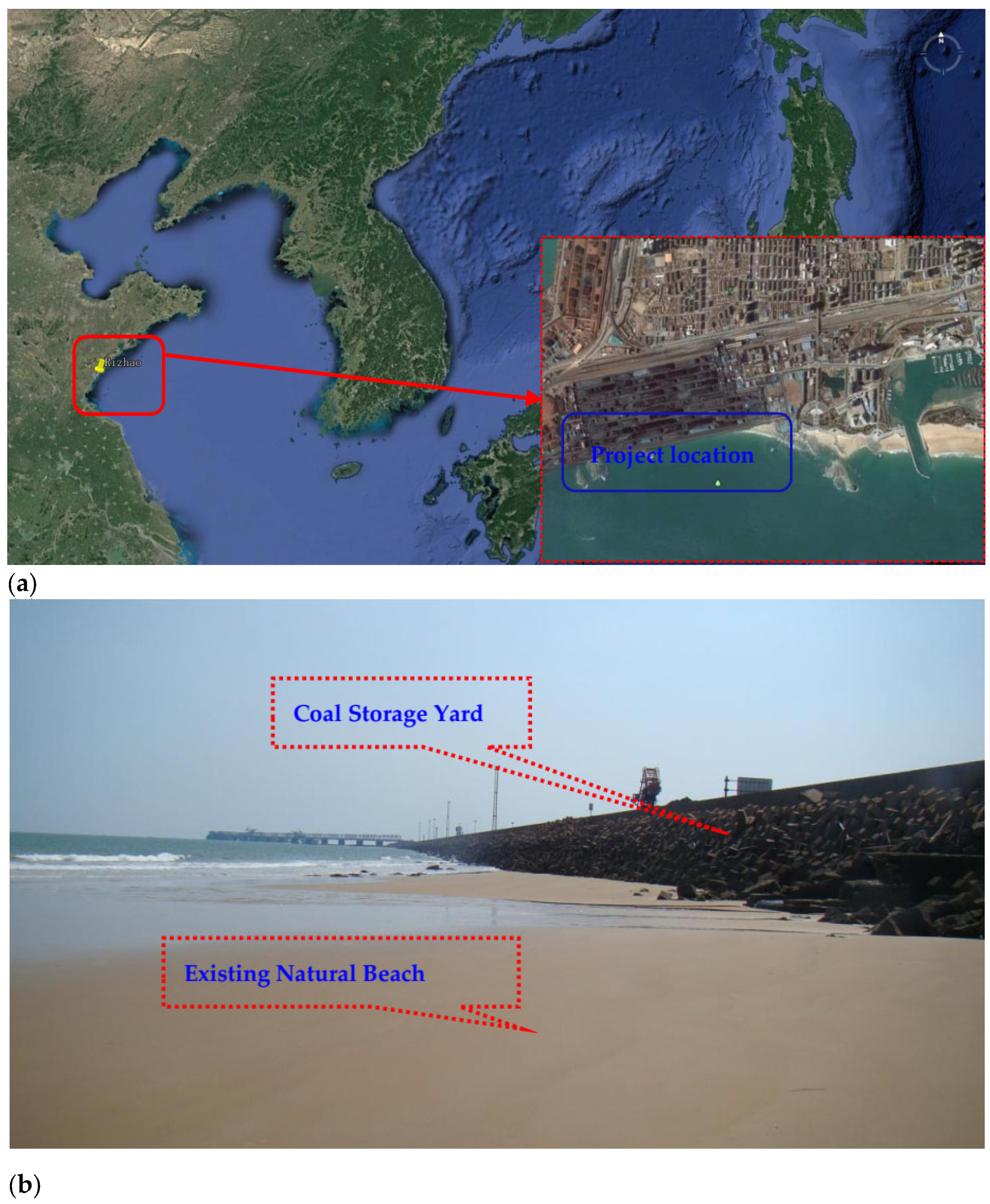
The current location of the proposed project is located in the bedrock cape area of an arc-shaped bay, with a small curvature on both sides of the bay. The shore section far from the cape is almost straight. In the early days of the coastline, there were beaches. Later, due to the reclamation of coal storage yards, the beaches were occupied by the yards. Currently, only a small area of beach has been preserved in the northern section of the coastline, as shown in Figure 1.

Figure 1.
Current situation of project location: (a) project location; (b) current conditions, sediment distribution at the project location.
2.1. Water and Sediment Environment in the Engineering Sea Area
According to the analysis of natural conditions in the engineering sea area [14]: (1) Waves are the main driving factor for beach sand movement. According to statistics from 1980 to 2011, tropical cyclones caused extreme weather exceeding Hs = 3.0 m a total of 16 times, mainly occurring from July to September (note: the measuring point is located 380 m in the ENE direction of the engineering location, at a depth of 12.9 m). Waves demonstrate a strong erosion of the sea floor, especially during the typhoon season, causing a severe cross-shore loss of sediment towards the sea; in addition, due to the NNW–SSE direction of the engineering coastline, the SSE–E direction waves have a strong impact on the coast, and the vertical revetment in the engineering area enhances wave reflection, resulting in there being no sediment deposition at the foot of the yard slope. The overall net transport trend of sediment in this coastal section is from south to north. (2) There is a residual current of 0.1–0.3 m/s in the engineering area (note: during the ups and downs of the spring tide) with a direction from north to south. When strong wave action lifts sediment from the seabed, the current transports this suspended sediment, causing further loss of sediment. (3) The terrain of the engineering shore section undergoes drastic changes, with an uneven distribution of reefs. In the reef area, the slope of the seabed is mostly between 1:5 and 1:50, and the local reef area near the shore reaches a steep slope of 1:1.5, which is not conducive to the retention of sediment.
Therefore, in the vicinity of straight beaches and in environments where strong waves and currents cause coastal sediment transport, in order to maintain the stability of the newly constructed artificial beach shoreline, it is necessary to design certain strength protection measures upstream and downstream of the beach for protection.
2.2. Necessary Conditions for Beach Formation
Research on protective technologies for sandy beach erosion. In recent years, more and more researchers have shifted from hard protection to soft protection techniques, or a combination of soft and hard protection [15,16,17]. The combination of artificial beaches and submerged embankments demonstrates a combination of soft and hard protection technology. Our laboratory has also conducted a large number of experimental studies on the combination of protective measures for different sandy coasts [18], and some of the results are shown in Figure 2.
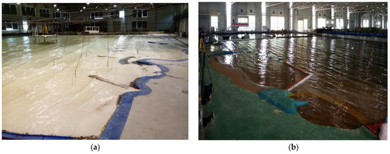
Figure 2.
Part of the results of research on beach protection measures in the laboratory: (a) combination test of spur dike and submerged dike; (b) combination test of sand barrier and submerged embankment.
Based on the hydrodynamic environment and current situation of this project, and in order to reduce the loss rate of sand on the beach and maintain the necessary conditions for the formation of the beach, the following three protective measures need to be implemented: (1) build a new breakwater on the southwest side of the project to reduce the direct impact of waves on the beach; (2) build sand-retaining dikes similar to spur dikes upstream and downstream of the beach, forming new headlands with the aim of reducing longitudinal coastal sediment transport; (3) based on the particle size of the sand, create a suitable beach slope to prevent lateral sediment transport.
Based on the protective measures for the artificial beach mentioned above, the optimal combination of schemes was obtained through numerical simulation prediction and physical model testing. The newly built artificial beach met the design objectives after practical operation on site.
3. Sand Barrier Case and Shoreline Shape Prediction
3.1. Calculation Theory of Balanced Coast in Cape and Bay
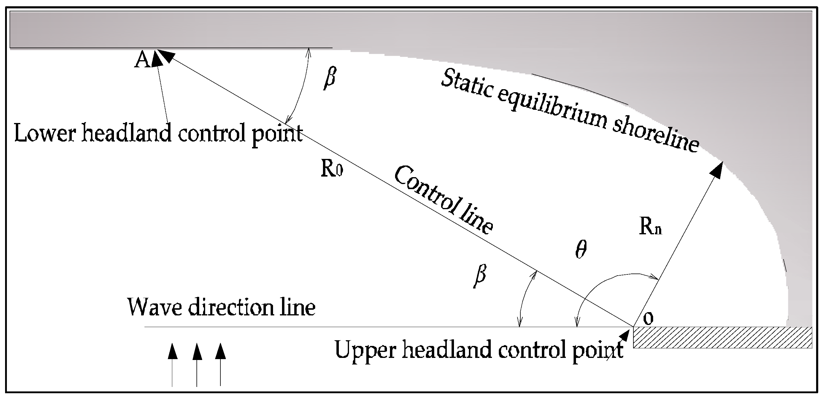
The theory of headland–bay equilibrium coast is to deduce the static stable shoreline shape under the conditions of no upstream supply of sand sources and control of upstream and downstream by fitting a large number of on-site beach shorelines and headland positions. According to Hsu and Evans [19], the on-site morphology of 27 actual coasts was fitted, and the expression is shown in Equation (1). Subsequently, Silvester and Hsu [20] further verified the rationality of the model.
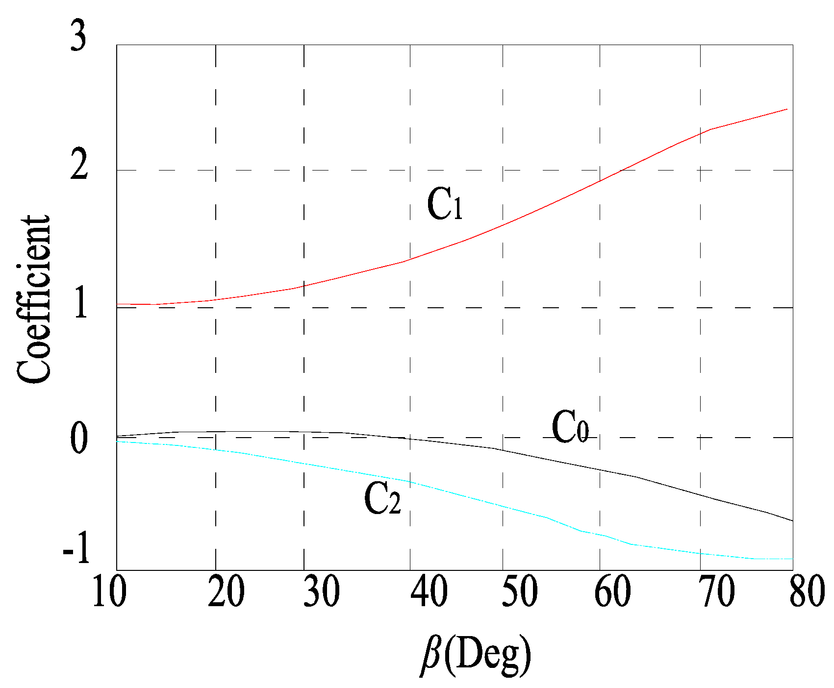
where is the radius of any pole (m), as shown in Figure 3; is the polar angle (deg); is the length of the control line (m); and is the angle between the crest line and the control line (deg), generally ranging from 10° to 80°. , , and are empirical coefficients and functions of , with values ranging from 2.5 to 1.0. For ease of use, the relationship curve between and can be fitted using Formulas (2)–(4), as shown in Figure 4, which can be directly used for reference.
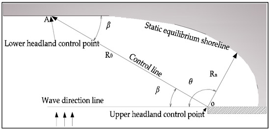
Figure 3.
Relationship between the parameters of the empirical formula for the headland–bay coast.
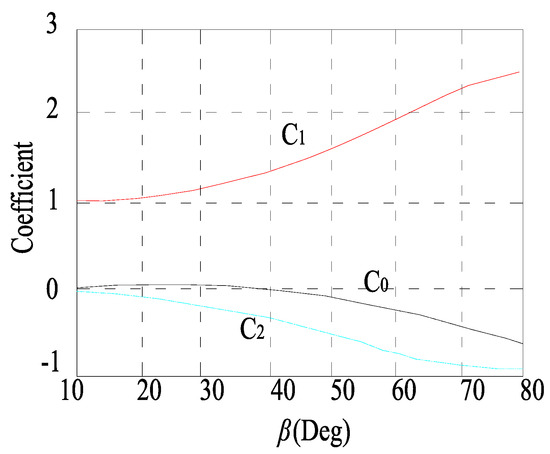
Figure 4.
Relationship between coefficients C and β.
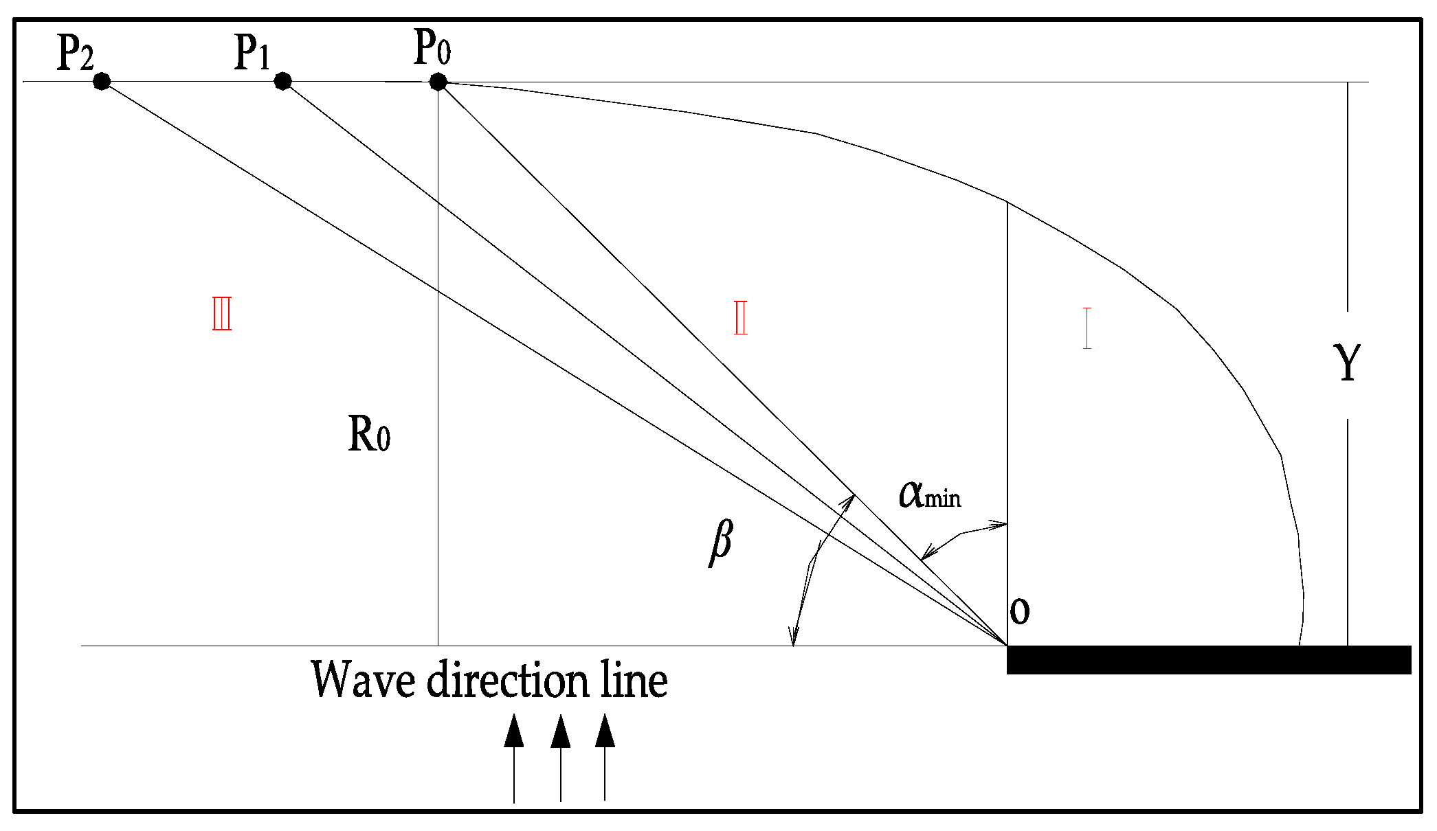
Determination of control points for the lower headland in Figure 3. González and Medina [21] derived corresponding calculation formulas, as shown in Equation (5). The relationships between the variables in the formula are shown in Figure 5. From the figure, it can be seen that in the equilibrium headland–bay empirical model, the line connecting two headlands is usually defined as the control line (commonly represented by R0), the point where waves diffract is defined as the upper headland, and the other headland where the tangent line segment is located is the lower headland. The incidental waves passing through the headland undergo refraction and diffraction, resulting in the uneven distribution of coastal wave heights. This means that refraction and diffraction cause waves entering the bay to have a coastal wave height gradient. Therefore, when calculating, the bay is first divided into three parts. The first part (note: I zone in Figure 5) is caused by the refraction and diffraction of waves, resulting in a coastal wave height gradient; the second part (note: II zone in Figure 5) comprises the coastal gradients of wave height caused solely by refraction; and the third part (note: III zone in Figure 5) is not affected by refraction and diffraction, and there is no coastal gradient of wave height. It is obvious in Figure 5 that the location of the lower cape point at P1 and P2 does not affect the incident conditions of the waves, and therefore does not change the shape of the headland. That is, the position of the lower headland point has no effect on the shape of the equilibrium headland–bay. P0 is the intersection point of the second and third parts at the shoreline, which is the endpoint of wave refraction. Therefore, this is the only confirmed point, which is the ”headland control point” in the equilibrium form model. The corresponding control line R0 is the line connecting P0 and the upper headland point (P0O), and Y is the maximum depression of the bay, which is the vertical distance from the upper headland point to the tangent of the bay, the angle between Y and the control line (P0O).
where , is the average wavelength corresponding to a large wave with a duration of 12 h in a year (m), and the corresponding period is the average period of a large wave with a cumulative frequency of 3%. The wavelength can be obtained from the dispersion equation. Therefore, the calculation formula for is shown in Equation (6).
where is the distance from headland to balanced shoreline (m), and αmin is the minimum angle from headland to equilibrium shoreline (deg).
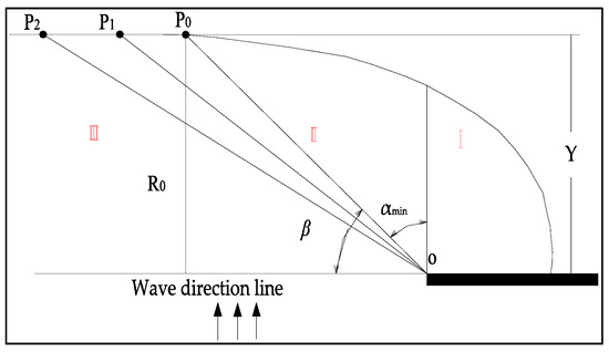
Figure 5.
Determination of the relationship between various variables in the location of the lower headland.
At present, the prediction model has been introduced into the “Guidelines for Coastal Engineering” [22], which provides a good reference for studying beach sediment movement and coastal protection engineering. At the same time, in order to reduce human labor, the prediction model was digitized into the MEPBAY [23] and SMC [24] calculation software, and the software model was tested using a large number of actual natural and artificial beach engineering cases, confirming its effectiveness. By comparing the applicable characteristics of MEPBAY [23] and SMC [24], this article chose MEPBAY software to use for calculating the equilibrium shoreline of artificial beaches.
3.2. Proposal of the Case and Analysis of Its Impact on the Balanced Shoreline of the Beach
3.2.1. Proposal of Cases
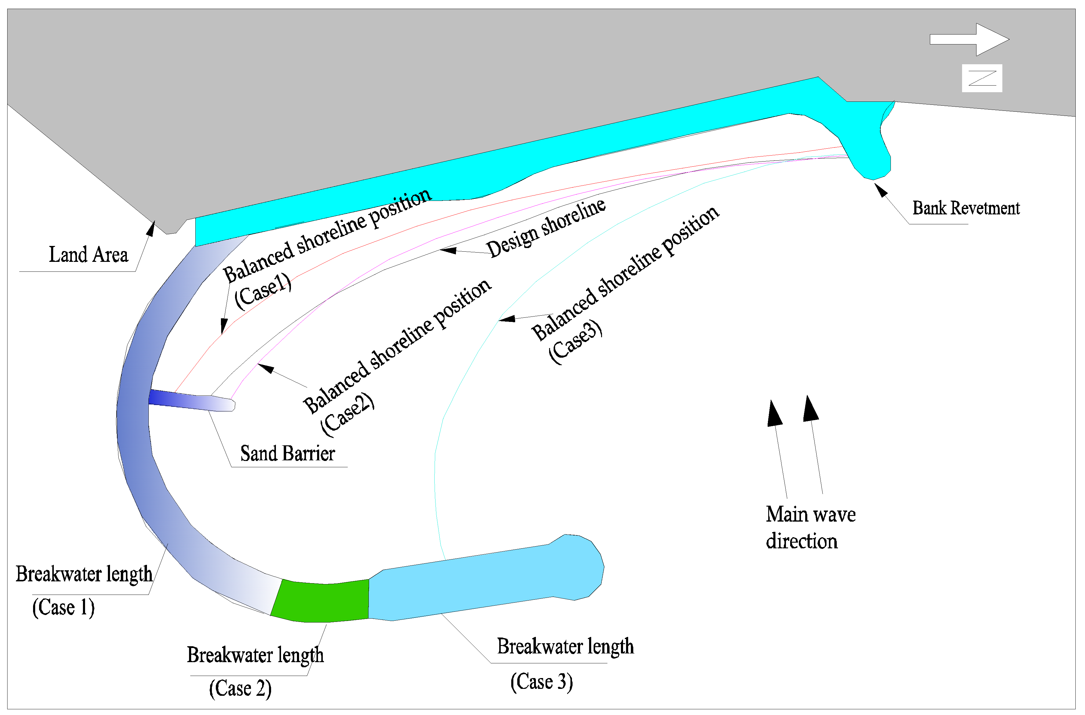
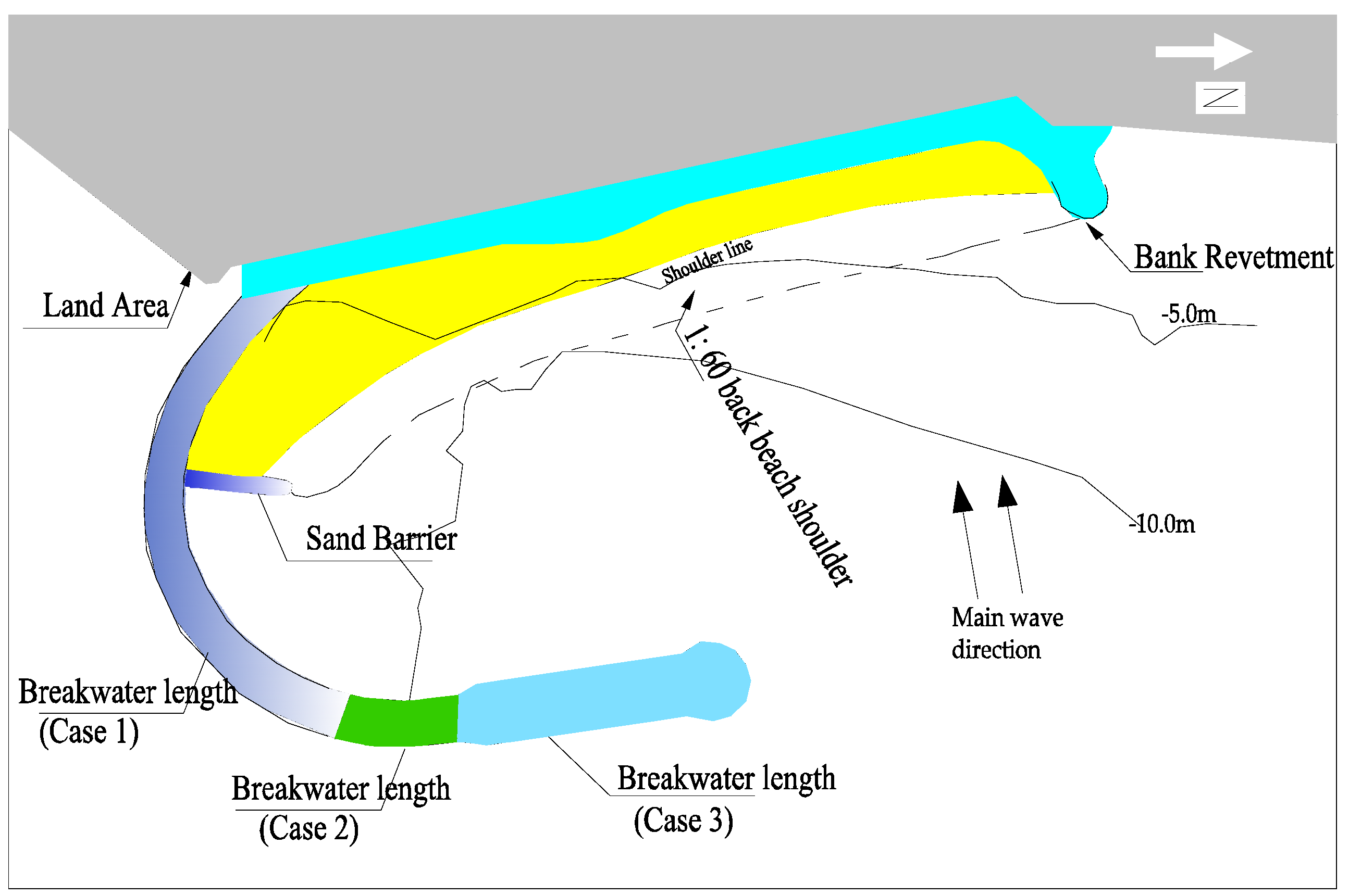
Based on the analysis of the actual situation of the above engineering locations, three protection schemes have been designed and proposed for the protection of newly constructed artificial beaches [25]: (1) case 1: design a curved sand-retaining embankment on the south side of the project area, with a length of 1220 m and a distance of approximately 1.0 km from the existing shoreline; (2) case 2: based on case 1, the embankment head extends northward to 1440 m, while the rest remains unchanged; (3) case 3: based on case 1, the embankment head extends northward to 2000 m, while the rest remains unchanged. The layout of each option is shown in Figure 6.
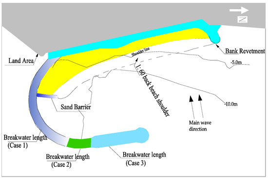
Figure 6.
Layout plan of three protection cases.
3.2.2. Proposed Artificial Beach Sections
(1) Firstly, calculate the sediment activity area by introducing the closure depth, which refers to the active sediment movement at a shallow depth where sediment activity is small or negligible. The calculation formula proposed by Hallermaier [26,27] is used, Formula (7):
where is the height of the nearshore wind wave with a frequency of 12 h/yr, which is 0.14% of the large wave height (m); is the corresponding period (s); is the closure water depth (m); and g is the acceleration of gravity (kg·s−2). Birkemeier corrected Hallemreier’s formula using high-quality field measurement data [28]: .
For this project area, based on the measured data from the open sea in 2002, the wave height sequence obtained from the wave model was used to calculate = 3 m, and the average closed water depth was calculated to be 4.7 m (note: the measuring point is located 380 m in the ENE direction of the engineering location, at a depth of 12.9 m). In areas with high slopes and bedrock terrain, affected by wave accumulation effects, the closed water depth was calculated to be 9–10 m.
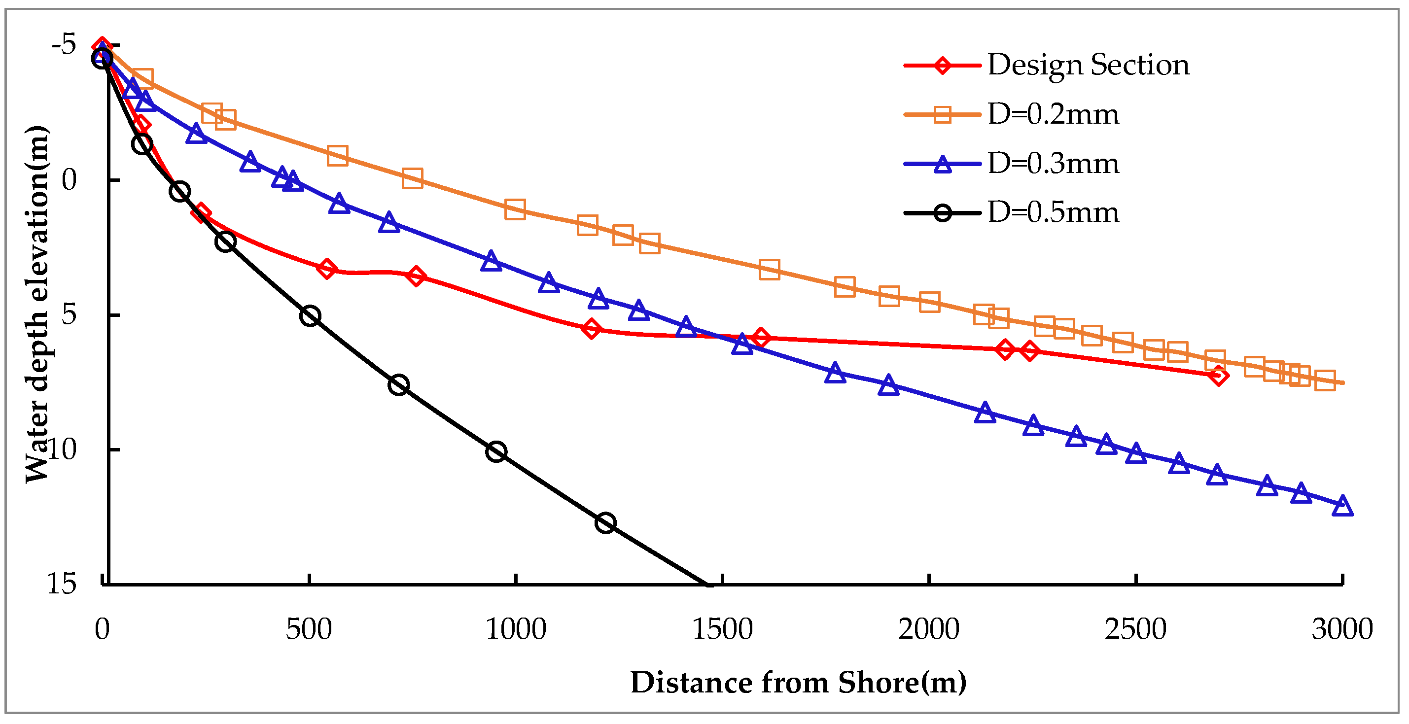
(2) Once again, Bruun [29] proposed a formula for calculating the beach sections, as shown in Equation (8). Calculations were conducted for the median particle sizes of D = 0.2 mm, 0.3 mm, and 0.5 mm on the beach, and three different particle size profiles were presented based on the closure depth of the beach, as shown in Figure 7. From the figure, it can be seen that after the deformation of the sand beach section with a particle size of D = 0.5 mm, the underwater section shape is basically consistent with the existing sand beach section on site.
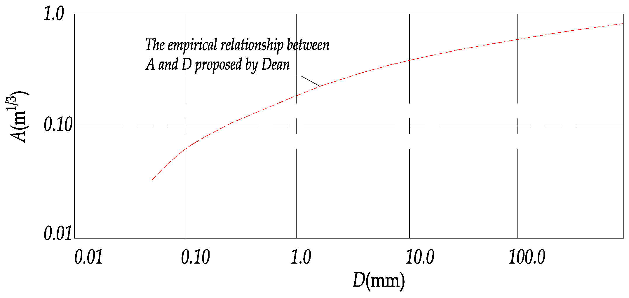
where represents water depth at the distance y from the coastline (m), and A represents the profile scale parameter (m−1/3). Dean [30] believes that A is related to the sediment particle size D, as shown in Figure 8.
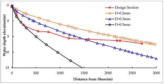
Figure 7.
Comparison of calculated beach equilibrium sections and measured sections.
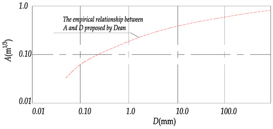
Figure 8.
The empirical relationship between A and D proposed by Dean.
The design of the beach profile is as follows: the slope of the foreshore beach is 1:60, and the width is 60 m; the slope of the back beach is 1:40, connecting with the mud surface on the sea side. At the same time, considering the sand source conditions of the project location where the sediment is laid, it is proposed to use the median particle size of D = 0.41~0.51 mm interval sediment for artificial beaches.
3.2.3. Prediction and Analysis of Beach Equilibrium Shoreline
Based on the three engineering proposals proposed in the design, as well as the profile of the beach, the MEPPAY model was used to predict the evolution of the shore and beach, and the results are shown in Figure 9. As shown in the figure:
- (1)
- Case 1: After the beach stabilizes, a portion of the beach can be retained on both the north and south sides (note: yellow part), while the erosion in the middle section is severe, and the narrowest dry beach is less than 20 m wide.
- (2)
- Case 2: After the beach stabilizes, most of the beach can be retained before the revetment. Compared to case 1, the reserved width of the balanced shoreline of the dry beach is large, indicating that the lengthening of the embankment has a significant diffraction effect on waves, which is beneficial for the stability of the beach. Slightly eroded beach on the north side: there is a trend of sedimentation near the sand barrier on the south side; there is still some erosion in the middle section, but the degree of erosion is weaker than case 1. The narrowest part in the middle can retain a dry sand beach of about 50 m in width.
- (3)
- Case 3: The dry beach shoreline continues to advance towards the sea compared to case 2. This indicates that case 3 has a significant shielding effect on waves and is beneficial for the stability of the beach. However, due to the breakwater being too long, a closed harbor is formed on the south side, and the southward waves entering the harbor are weak, resulting in the overall southward transport of sediment. The south side is heavily silted, which is not conducive to the hydrophilic landscape and may also pose a risk of mudding.
Based on the above analysis, case 2 was designed as the recommended scheme and further physical model experiments were conducted to verify the rationality of the recommended case.
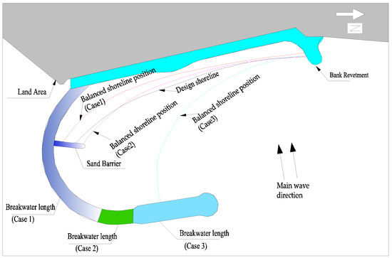
Figure 9.
Plan layout and equilibrium shoreline prediction results.
Figure 9.
Plan layout and equilibrium shoreline prediction results.
4. Model Tests
4.1. Experimental Design and Environmental Simulation
4.1.1. Model Design
(1) Analysis of sediment movement characteristics on the shore: The sediment movement characteristics in the sea area are mainly driven by wave and tidal forces. Therefore, an analysis was conducted on the sediment movement characteristics;
① Firstly, the Zhang Rui-jin Formula (9) [31] was used to calculate the starting flow velocity under tidal power, and 0.49 m/s was obtained. Compared with the tidal power in the engineering sea area, the maximum tidal flow velocity was 0.35 m/s, indicating that the tidal power is not sufficient to cause the bed sediment to start
② Using Formula (10) of the “Hydrological Code for Ports and Waterways” (TJS145-2018) [32] to calculate the starting wave height of sediment caused by waves again, it was found that when the water depth is 2.0 m, the starting wave height only needs to be 0.40 m. The probability of the wave height exceeding 0.5 m in the engineering sea area in one year is about 67%, indicating that the main starting force of sediment is wave power. Therefore, when designing the model, the starting force of sediment is mainly wave power, taking into account sediment deposition:
where is the starting velocity of sediment (m·s−1), is the sediment density (kg·m−3), is the gravity of water (kg·m−3), is the starting wave height of sediment (m), is the starting wavelength (m), and D is sediment grain size (m−3).
(2) Test simulation scope: Based on the test purpose and the size limitations of the test pool, the scale is used as a normal model, and the relationship between various physical scales is summarized in Table 1.

Table 1.
Summary of physical scale relationships.
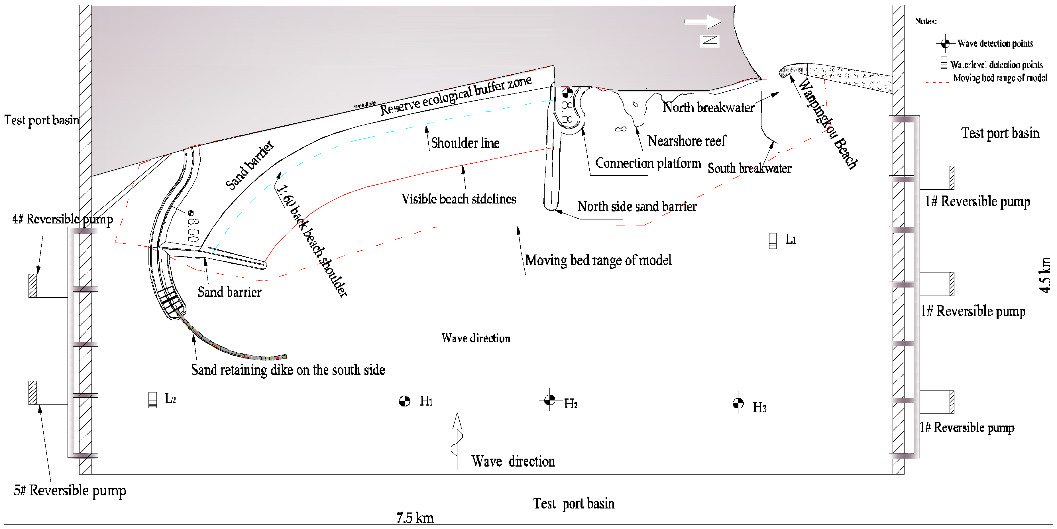
Testing at a length of 75 m × width 45 m, the simulation is conducted in a 1.3 m deep comprehensive water tank, simulating the range of the sediment moving bed: horizontally from the shoreline to the water depth surrounded by the south and north sand barriers, and longitudinally from the 1.5 km range outside the south and north sand barriers (see Figure 10).
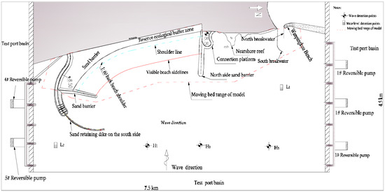
Figure 10.
Model layout and measurement point layout.
(3) Model sand selection: Based on the hydraulic characteristics of the prototype sand and the similarity in scale, the laboratory selects a specific gravity of 1.30 × 10³ kg/m3 plastic sand with a median particle size of 0.45 mm to be used as the model sand.
(4) Test equipment and measurement point arrangement: The wave-making machine adopts a rocking plate type. The wave-making ability is the maximum wave-making depth of 0.8 m, the wave height of 0–0.3 m, and the period of 0.5–4.0 s. To reduce wave boundary reflection, wave absorbers are installed around the port basin. The wave type adopts irregular waves with a JONSWAP spectrum. At the same time, in order to prevent secondary reflection caused by long-term wavemaking, the experiment adopts segmented wavemaking. Wave calibration and monitoring are measured using three H1–H3 wave height sensors arranged at the model boundary, as shown in Figure 10; the tidal system at both ends of the model adopts reversible variable frequency speed regulation closed-loop water level control to simulate the process of rising and falling tides, and L1 and L2 are set for tidal level monitoring, as shown in Figure 10. The measurement of beach profile erosion and sedimentation deformation is carried out using a 3D laser scanner for scanning and processing. During the experiment, waves, tidal systems, wave heights, and water levels are collected using self-developed software for control and data collection.
4.1.2. Environmental Simulation and Methods
(1) Method for determining the dynamic conditions of model validation: Using perennial waves and data from wave stations in the engineering area from 1990 to 2011, based on the representative wave height and direction calculation Formulas (11) and (12) specified in the “Technical Specification for Water Transport Engineering Simulation Testing” (JTS/T231-2021) [33], it can be calculated that = 0.83 m, = 4.2 s, and the representative wave direction = 89.7°. Referring to the experience of Xia Yimin [34] and other sediment models [35,36,37], the model test generally requires a wave height of no less than 0.015 m and a period of no less than 0.6 s. Based on the calculation of the experimental scale relationship, the initial wave height is slightly smaller than the required wave height. Therefore, during the verification experiment, the requirement of increasing the wave height and period to general was adopted; that is, the wave element adopts a distorted scale, but the final goal of the model is to verify that the results of terrain erosion and sedimentation changes meet the specifications, thereby ensuring that the model design parameters are reasonable and the conclusion is reliable.
where represents the wave height (m), represents the wave direction (deg), is the effective wave height greater than the starting wave height i of sediment (m), is the frequency of wave height and direction above the i value (t−1), and is the wave direction angle above the i value (deg).
Test water level simulation: a cycle process is adopted from low water level (+1.09 m) → average water level (+2.62 m) → high water level (+4.10 m) → average water level (+2.62 m) → low water level (+1.09 m).
(2) Determine terrain verification data: Using the north side of the project location, where the south and north breakwaters were built in 2005, collect the results of erosion and sedimentation changes on both sides of the breakwater and within the waterway from 2005 to 2015. Obtained: Shallow erosion along the 2 m isobath at the root of the north breakwater, with an amplitude of approximately 0.1–0.5 m; the depth of the 5 m contour line at the root of the south breakwater is shallow erosion, with an erosion amplitude of about 0.5~1.2 m. The sedimentation amount in the waterway is about 0.1–0.2 × 10⁴ m3/yr; these can be used as model validation data.
(3) Model validation test: Using the above dynamic conditions and terrain data, model calibration was carried out to obtain the results of erosion and sedimentation changes in the validation area of the model, as shown in Table 2 and Figure 11. By comparing the results of erosion and sedimentation changes between the model and the site, it can be seen that the erosion and sedimentation changes in the root of the breakwater and the channel are basically the same as the original source, indicating that the design of the sediment model and the selection of model sand are reasonable. Therefore, further experiments can be carried out in the next step of the case.
Table 2.
Comparison results of topographic erosion and sedimentation between prototype and model tests.
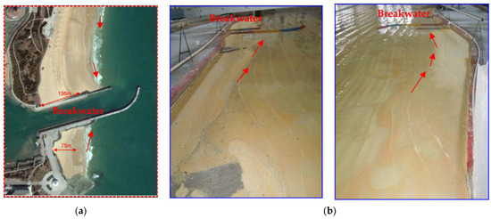
Figure 11.
Comparison results of sediment erosion and sedimentation deformation at the roots of breakwaters on both sides of the waterway. (a) On site; (b) model test. (note: The arrow in the figure indicates the direction of sediment transport).
(4) The determination of the time scale for erosion and sedimentation in the experiment: First, the on-site sediment transport results on the beach are used [25]. Then, by arranging multiple sediment collection channels in the vertical shoreline direction on the model, the sediment transport on the beach is obtained. Then, the sediment transport similarity relationship equation is used to obtain the sediment transport scale. Based on the similarity relationship of erosion and sedimentation time, the model erosion and sedimentation time scale can be obtained. Using this scale, it can be inferred that the on-site time is 1 year, and the model requires 13.6 h.
4.2. Test Results and Analysis
4.2.1. Recommended Case Test
After a year of continuous wave action, the sand and sediment movement on the beach mainly moves from south to north, resulting in the loss of sediment on the beach surface (note: sand and sediment loss here refers to the transport of sediment on the surface of the beach to areas outside the beach profile after wave action. Without human intervention, it cannot be transported to the surface of the beach again). The methods of sediment loss can be roughly divided into three categories. The first category is that sediment is transported to the scenic area by bypassing the north sand barrier, the second category is that sediment is transported to the root area of the breakwater by bypassing the south sand barrier, and the third category is that sediment is transported horizontally to the deep water area at the foot of the beach profile slope. The specific loss results are shown in Table 3. In addition, due to the loss of sediment in the beach profile, the design width of the beach (60 m) has changed, with a maximum variation width of 30 m, a minimum variation width of 5 m, and an average variation width of 20 m. The specific results are shown in Table 3. The sand beach profile transport and loss are shown in Figure 12.
Table 3.
Test results of sediment changes under design case 2.
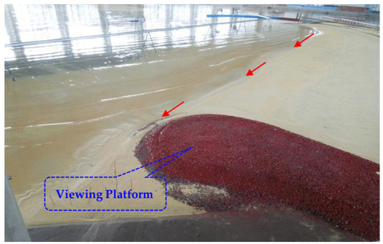
Figure 12.
Sediment movement under wave action for case 2. (note: The arrow in the figure indicates the direction of sediment transport).
4.2.2. Optimization Case Test
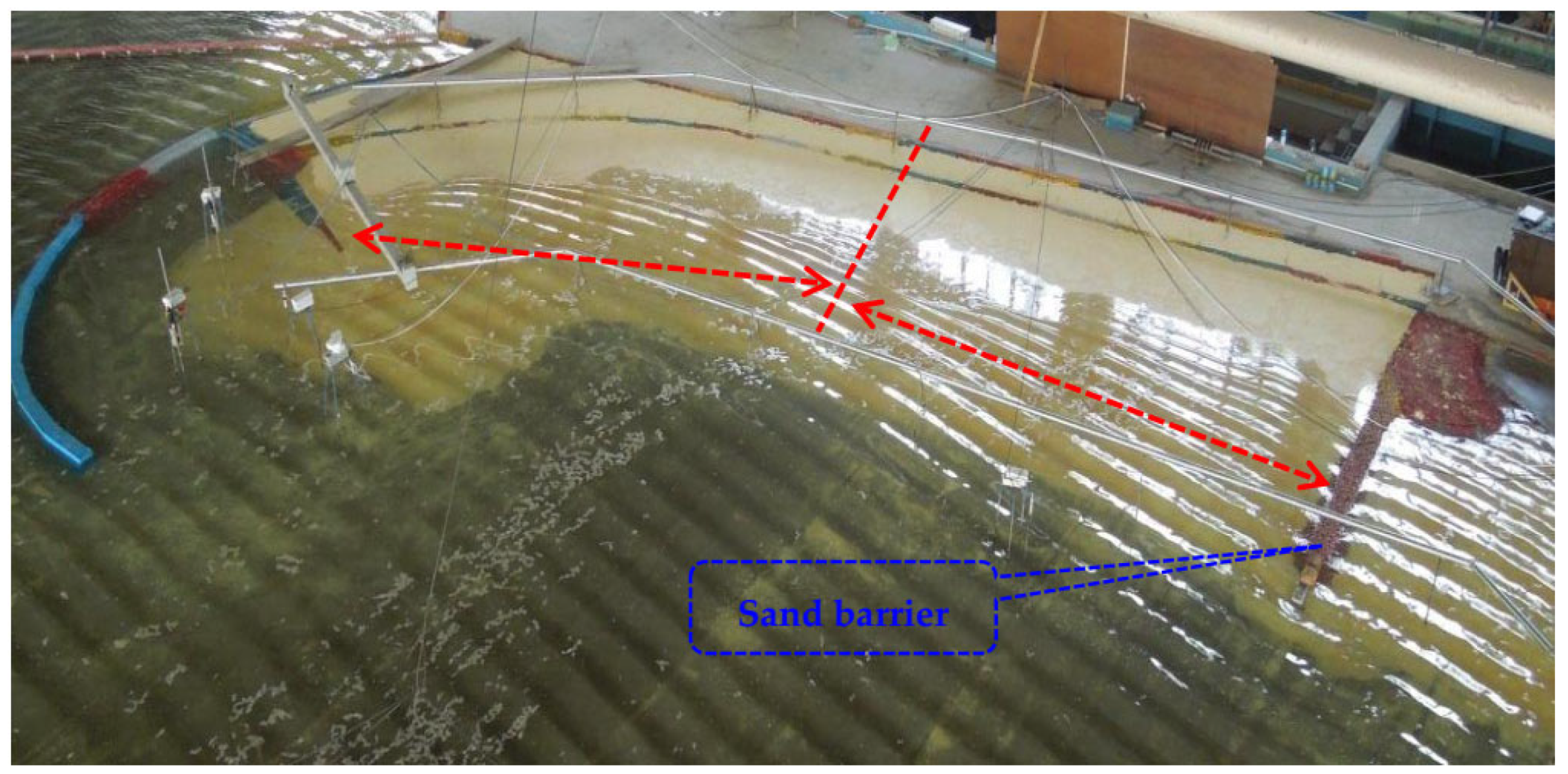
Based on the insufficient length of the north sand barrier and the impact of sediment bypassing the embankment head on the surrounding scenic areas, the recommended length of the north sand barrier has been optimized, as shown in Figure 13. At the same time, based on the previous calculation of a closed water depth of 9–10 m, experiments were conducted to increase the length of the north sand barrier to 250 m, 280 m, 300 m, and 400 m, individually. After a year of continuous wave action, the results of sediment loss on the beach surface are shown in Table 4 (note: the classification method for sediment loss is the same as Table 3). From the results in the table, it can be seen that as the length decreases, the amount of sediment loss towards the scenic area decreases significantly. Similarly, with the loss of sediment on the surface of the beach, the designed dry width of the beach changes. The statistical results are shown in Table 4. From the results in the table, it can be seen that the maximum variation width is 30 m, the minimum variation width is 0 m, and the average variation width is 12.5 m. Comparing the results of beach changes under different lengths of sand barriers, and considering the sediment activity boundary near −5.0 m in the northern region, as well as the economic and environmental impact of the project, the recommended length of the north sand barrier in the experiment is 300 m, and the water depth at the head of the barrier is about 8.5 m.

Figure 13.
Optimization of the length of the north sand barrier and the situation of sediment movement under wave action.
Table 4.
Test results of sediment changes under different lengths of sand barriers.
4.2.3. Recommended Beach Sections
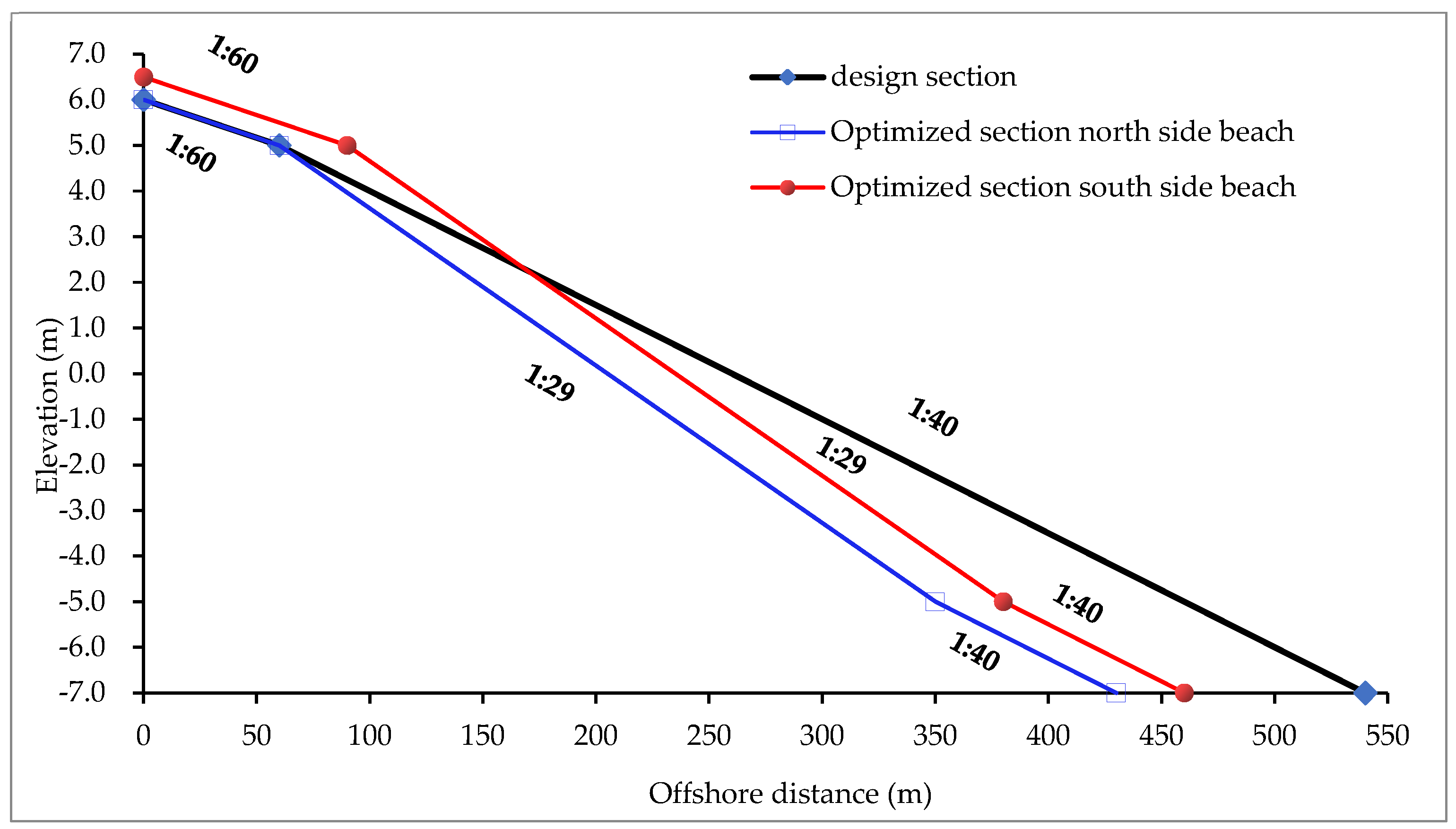
Based on the optimization case, the deformation and stability results of the beach are obtained as follows: ① The section from the north sand barrier to the middle of the beach from the shore to the sea side is 0 m to 60 m, with a slope of 1:60 and an elevation of +6.0 m to +5.0 m; 60–350 m, with a slope of 1:29 and an elevation from +5.0 m to −5.0 m; and 350 m to muddy surface connection, with a slope of 1:40 and an elevation of −5.0 m to the muddy surface. ② The section from the middle of the beach to the south sand barrier is 0–90 m from the shore to the sea side, with a slope of 1:60 and an elevation of +6.5 m to +5.0 m; 90–380 m, with a slope of 1:29 and an elevation from +5.0 m to −5.0 m; and 380 m to the muddy surface connection, with a slope of 1:40 and an elevation of −5.0 m to muddy surface. Therefore, it is proposed to optimize the beach profile, with the middle as the dividing line, designed according to two different profiles. At the same time, the profile is divided into three slopes. Compared with the design, it can save 12% in sand replenishment and save CNY 2 million in project costs. The optimized profile shape formula is shown in Figure 14.
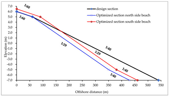
Figure 14.
Comparison results of beach profile design and optimization (note: the positive and negative elevations of the beach profile in the figure are calculated from the local theoretical reference plane of the engineering location, which is the 85 elevation reference plane in China).
4.2.4. Determination of Beach Maintenance Cycle
The construction of artificial beaches is usually not a one-time effort and requires regular maintenance. For the beach maintenance cycle standard of this project, the evaluation is mainly based on the comfort level of tourists on the beach, and two methods are proposed in the experiment.
(1) The width standard after dry beach erosion.
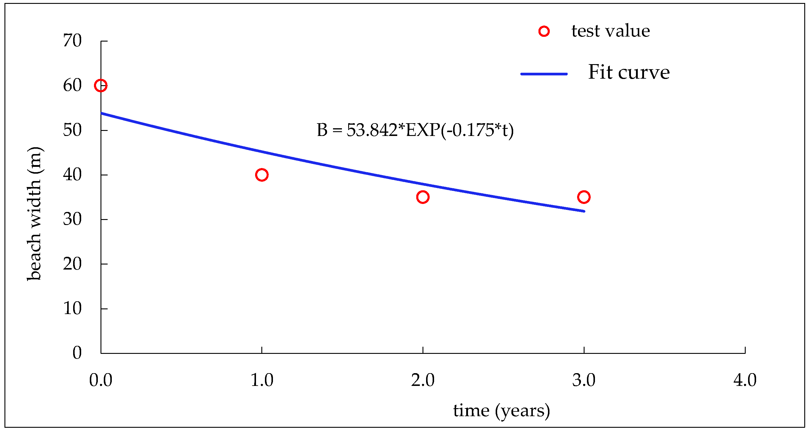
This design proposes dry beach erosion on high beaches, with a minimum width of B no less than 30 m. Based on the experimental results of the optimization scheme, the relationship was obtained between the maintenance period t and the average dry beach width B after erosion, as shown in Figure 15. According to the empirical Equation (13) obtained from the graph fitting, and calculated based on Equation (13) and maintenance standards, in the fourth year, the artificial beach needs to start maintenance.
where B is the width of the beach shoulder (m), and t is the continuous action time of the wave (t).
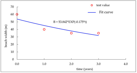
Figure 15.
Relationship between beach width and wave action time.
(2) The length of the sand-blocking embankment to the north is the standard for complete sand-blocking.
To protect the requirements of the northern scenic area, the standard is to ensure that no sediment is transported around the head of the sand barrier towards the scenic area. We calculated Formulas (14) and (15) using the “Hydrological Code for Ports and Waterways” (JTS145-2022) [32], and combined them with physical model tests to determine the sediment transport volume from south to north, 3.6 × 10⁴ m3, and taken into Equations (14) and (15), the maintenance cycle is calculated to be 5 years.
where is the fully effective sediment retention time of the embankment (t), is the fully effective sediment retention length of the embankment (m), is the sedimentation angle (deg), is the sediment transport rate along the upstream coast of the siltation area (m3·s−1), is the deformation height of the beach profile (m), and is the angle of wave incidence at the depth of the starting water of sand and sand on the beach (deg).
Based on the above two evaluation methods, in order to ensure the comfort of tourists on the beach, the artificial beach needs to be maintained after 4 years of construction.
4.2.5. Verification and Analysis after Beach Implementation
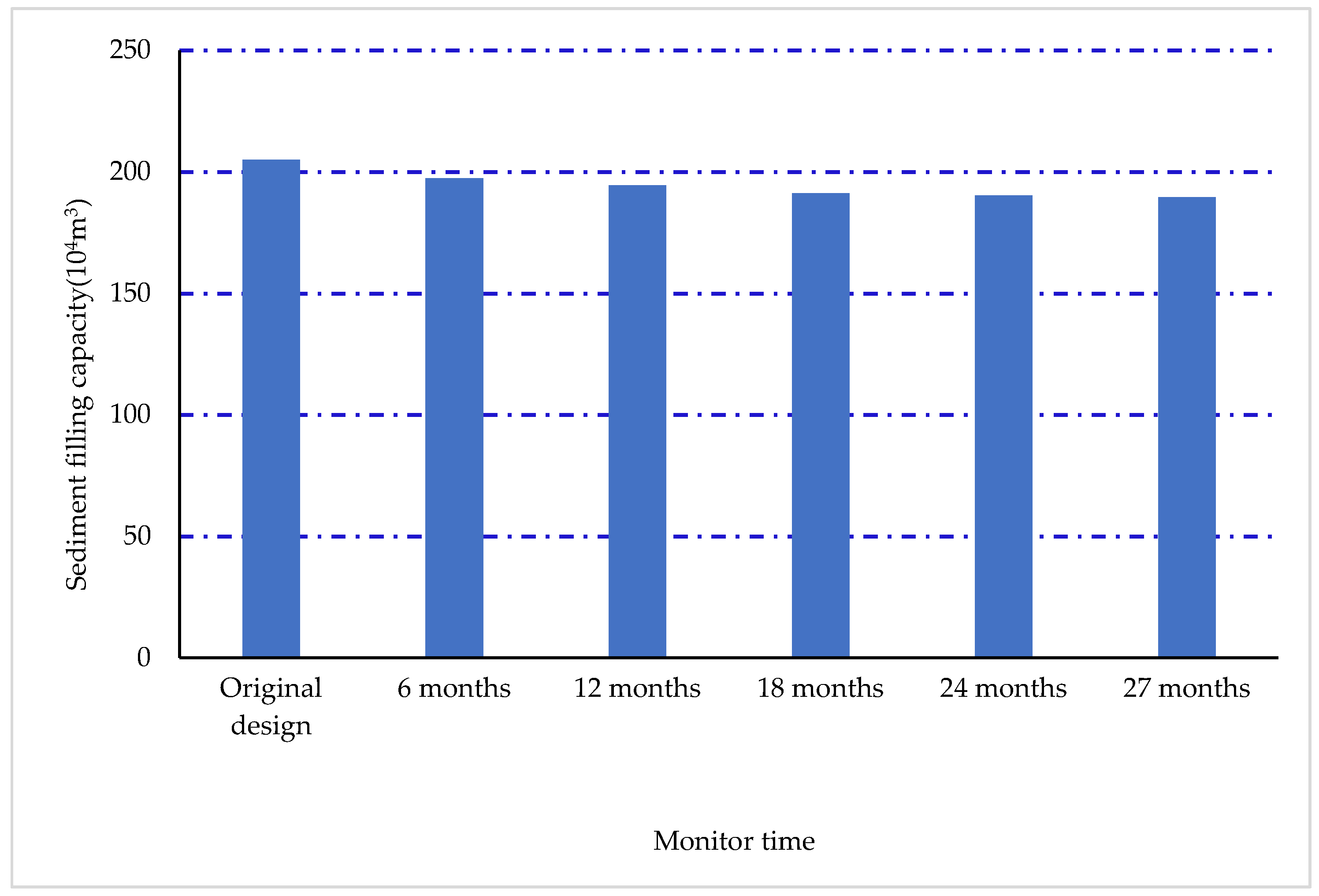
After the construction of the beach, on-site exploration and monitoring revealed that (1) erosion occurred in the central area, sedimentation occurred at the roots of the sand retaining walls on both sides, and there was a certain degree of sand transport in the north–south direction, with an annual net sand transport of about 3.6 × 10⁴ m3. (2) After continuous monitoring for 27 months, the sediment loss amount was about 10% of the total amount. The sediment loss amounts at different periods are shown in Table 5 and Figure 16. At the same time, according to the results of the table and figure, the erosion rate decreased after 18 months, indicating that the industrial beach began to transition to a stable state. (3) The position of the middle section has basically reached the result of sand transport balance, indicating that the sand retaining embankment has played its role in sand retention, and the constructed beach line has almost remained unchanged. This indicates that the groin has a good shielding effect on the beach, and the shoreline layout is reasonable. It also confirms that the selection of the beach equilibrium shoreline using the theory of headland–bay equilibrium coast is reasonable and effective.
Table 5.
Residual sediment volume at different times after the construction of artificial beach (unit: 104 m3).
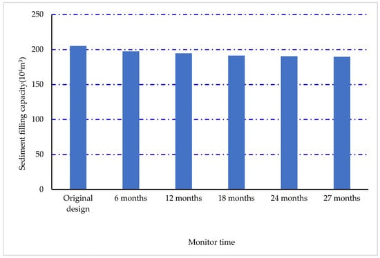
Figure 16.
Residual sand volume of artificial beach at different periods.
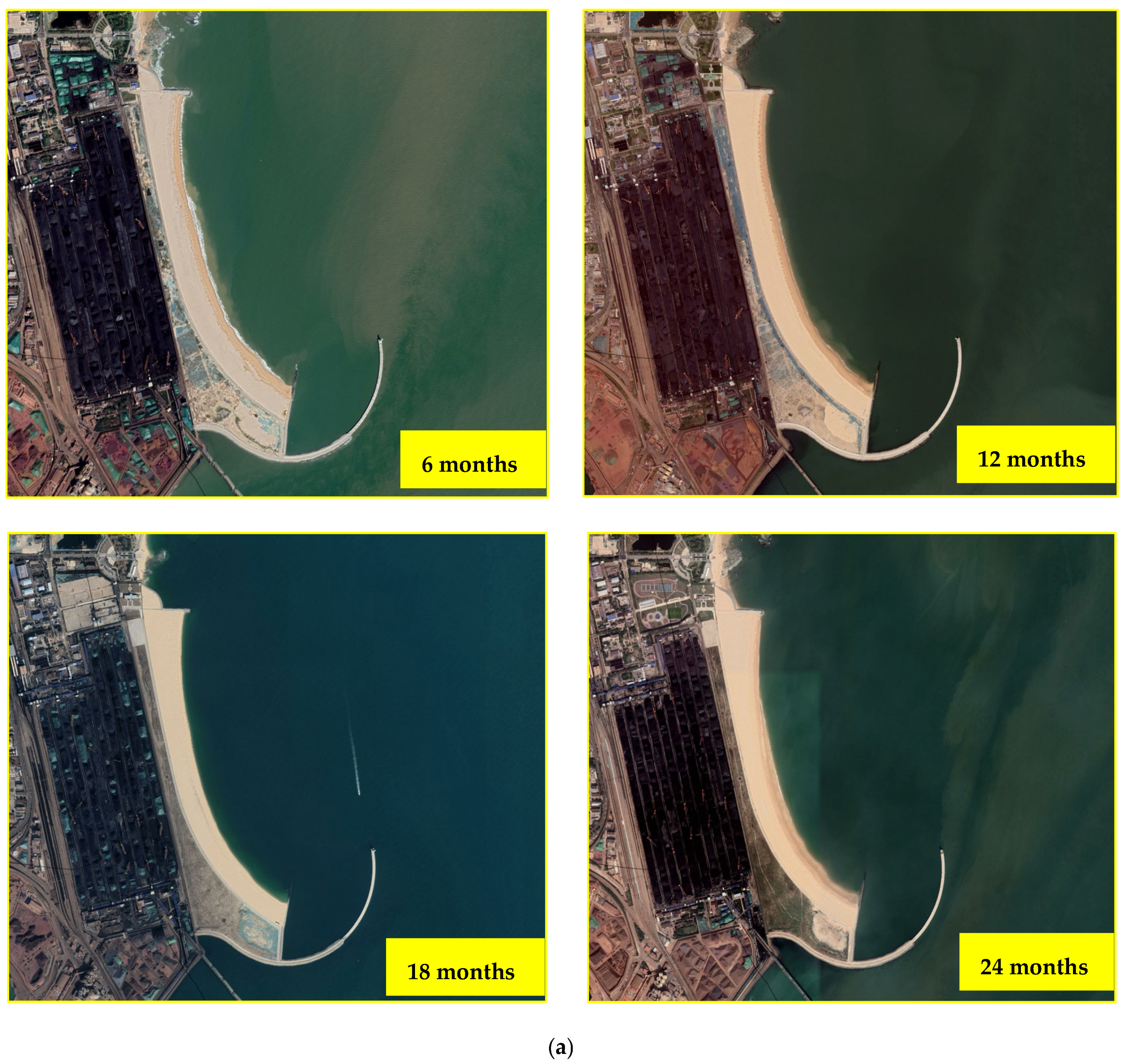
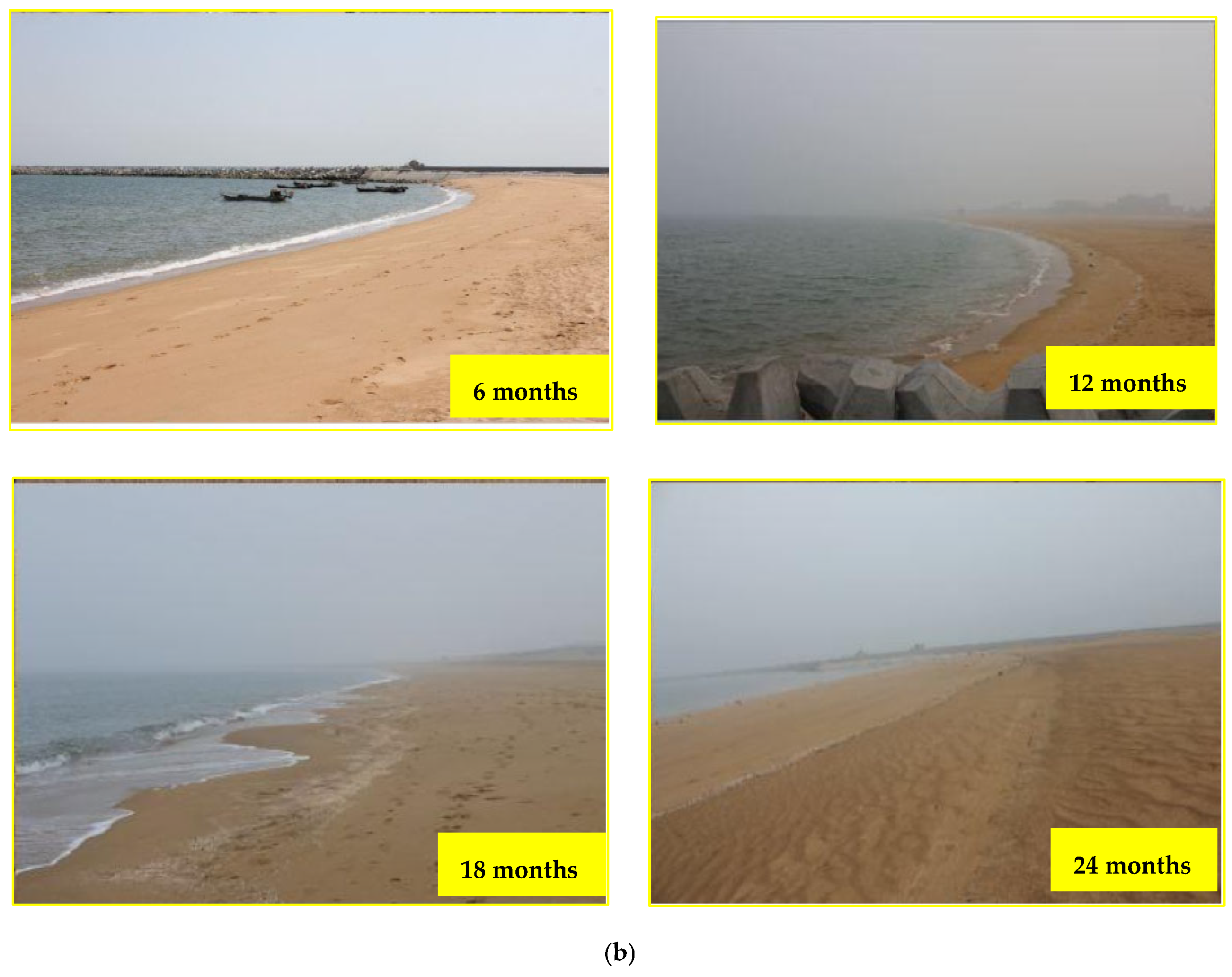
Through the comparison and analysis of the historical satellite images of the newly built beach and the on-site typical beach profile monitoring (see Figure 17), it was found that the profile changes in the beach are relatively small, and the shoreline has basically reached a dynamic equilibrium state, achieving the design purpose.

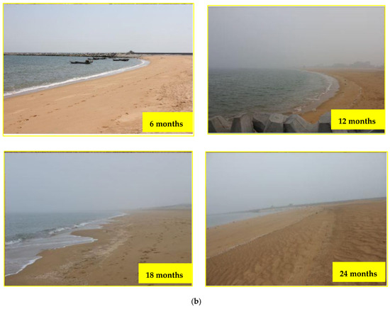
Figure 17.
On-site beach operation after 24 months: (a) satellite monitoring map of beach shoreline changes; (b) monitoring map of typical beach profile changes.
5. Discussion
(1) There is a deviation between the prediction of stable shoreline morphology based on equilibrium theory and physical model experiments. The main reason is that the parabolic type of equilibrium shoreline theory is applicable to the stable shoreline morphology formed by long-term dynamic changes in beaches, and cannot reflect the short-term dynamic evolutionary process of beaches. After the construction of artificial beaches or artificial structures is completed, the beach needs to undergo a period of dynamic changes in order to reach the final stable shoreline state. This dynamic change process involves complex factors, including the effects of tidal currents and wave forces on the beach, the refraction and diffraction of waves by natural headlands or artificial structures, water depth, terrain, profile slope, sediment particle size, and other factors. In addition, the MEPBY model is suitable for engineering evaluation, especially during the pre-design phase. Therefore, considering the deviation between the two, it is recommended to use the theory of headland–bay equilibrium coast, as well as comprehensive model tests or on-site verification, to further optimize the equilibrium theory for predicting the shoreline. This can provide guidance for improving the artificial beach and effectively save construction and maintenance costs.
(2) For beach maintenance, the experiment only proposed maintenance cycles under normal sea conditions. However, in extreme sea conditions, where astronomical tides correspond to waves with a return period of 50 years, typhoon waves mainly erode high beach sediment and accelerate the erosion and retreat of the dry beach width. That is, after a typhoon enters, the beach needs to be immediately maintained. Therefore, regular monitoring and timely maintenance of the beach should be strengthened to avoid the formation of secondary disasters.
(3) In the process of conducting physical sediment model experiments, the research focus is on preventing or reducing beach erosion. Therefore, the model adopts a normal scale to grasp the sediment movement mainly caused by wave power, ignoring other factors. Through verification with the on-site erosion and sedimentation positions and changes in erosion and sedimentation, under the condition that the error between the two meets the specification requirements, the erosion and sedimentation time scale is obtained. Based on the above, scheme experiments are carried out. The experimental results have been verified on-site, indicating that the overall design of this experiment is reasonable. Therefore, for sediment model experiments, it is recommended to use a combination of model and on-site monitoring methods as much as possible in order to accumulate experience for model experiments and provide guidance for the next experiment.
(4) Due to the influence of physical model testing sites, time, and funding, most beach engineering case planning only uses numerical simulation methods to evaluate the cases, such as the planning of some artificial beach projects in Yantai and Hainan provinces [38,39]. Some beach projects also use numerical simulation and physical model testing research methods but, due to the lack of on-site monitoring equipment and relevant professionals, there is a lack of on-site monitoring after engineering construction, and further verification and promotion of research results are lacking; for example, in the study of some beach protection projects in Fujian and Zhejiang provinces [5,40]. The research results of this study fully utilize the combination of numerical simulation and physical model experiments, using satellite images and typical profile monitoring methods to conduct on-site monitoring of the beach after construction for 2 years. The results of sediment loss and changes in the width of the dry beach are obtained, further supporting the research results and having broad prospects for promotion and application.
6. Conclusions
This article is based on the theory of the headland–bay equilibrium coast and takes the artificial beach project of the Rizhao Port’s “Return to Sea” project as an example to explain the application effect of this theory in the design of equilibrium shorelines in artificial beaches. It also analyzes the design parameters and corresponding balanced shoreline shapes of the protective engineering and uses physical model experimental research methods to further demonstrate the proposed recommendations. The following main conclusions were obtained:
(1) The artificial beach project lacks sediment supply from upstream and offshore sources, and the shoreline shape will be reshaped under wave action to achieve static equilibrium. Therefore, it is more appropriate to use the theory based on the curved equilibrium bay of the headland–bay for the simulation of its equilibrium shoreline. (2) Based on the analysis of the beach equilibrium shoreline under different protection cases, case 2 is superior to other cases. The rationality of the case was further optimized through physical model experiments and based on the implementation of different functional standards for artificial beaches; a reasonable maintenance cycle was proposed. Based on the situation of sand and sediment loss on the beach, a differentiated design was proposed for the artificial beach section. (3) After 27 months of implementation of the artificial beach, on-site monitoring and statistics showed that the sediment loss was less than 10% of the total amount, meeting the design purpose. This confirmed the effectiveness of the theory of the headland–bay equilibrium coast, combined with model experiments, in the protection engineering of the artificial beach and the design of the equilibrium coastline. It achieved good economic, social, and ecological environmental benefits, and has broad prospects for promotion and application. (4) This test was only conducted under normal sea conditions, and for extreme sea conditions, it is recommended to maintain the beach to avoid the formation of a second disaster. (5) There is a deviation between the prediction of stable shoreline morphology based on the equilibrium theory and physical model tests. It is recommended to use comprehensive model tests or on-site verification to further optimize the equilibrium theory prediction of shorelines and ensure that the scheme reaches the optimal level.
Through the results of this research, reference and guidance can be provided for the construction of similar artificial beach projects from the following aspects: (1) protective measures for the plane layout of newly built sand barriers on both sides of the beach that are larger than the width of the beach in order to ensure the stability of the beach; (2) the slope of the beach profile should be designed at 1:30 as much as possible to reduce sediment loss; (3) the maintenance cycle of the beach can be determined based on the standard of retaining the width after erosion of the dry beach, which can ensure the reasonable use of the beach; and (4) for the preliminary planning of the new project, a combination of numerical simulation and physical model testing should be used as much as possible for argumentation in order to make the scheme selection more reasonable. After the construction of the project, regular monitoring should be adopted to ensure that the beach can serve people for a longer period of time.
Author Contributions
Model design and testing, paper preparation, sediment erosion, and sedimentation changes data processing and analysis, writing—original draft, L.G.; analysis of the experimental datasets; methodology, the conception of the research, H.C. and S.C.; writing—review and editing, Y.L.; funding acquisition, Y.L. and S.C. All authors have read and agreed to the published version of the manuscript.
Funding
This study was financially supported by the National Natural Science Foundation of China (52039005, 52001149); special fund for central scientific research institutes (TKS20230505, TKS20230515); and National Key R&D Program of China (2022YFB2602301; 2022YFE0104500).
Institutional Review Board Statement
Not applicable.
Informed Consent Statement
Not applicable.
Data Availability Statement
Data sharing is applicable to this article, as new data were created or analyzed in this study.
Acknowledgments
This physical model test was conducted in the experimental harbor basin of the Tianjin Research Institute for Water Transport Engineering.
Conflicts of Interest
The authors declare no competing interest. The corresponding author is responsible for submitting a competing interest statement on behalf of all authors of the paper.
References
- Halligan, G.H. Sand movement on the New South Wales coast. Proc. Limnol. Soc. N. S. W. Aust. 1906, 31, 619–640. [Google Scholar]
- Davies, J.L. Wave refraction and the evolution of shoreline curves. Geogr. Stud. 1959, 5, 1–14. [Google Scholar]
- Silvester, R. Stabilization of sedimentary coastlines. Nature 1960, 188, 467–469. [Google Scholar] [CrossRef]
- U. S. Army Engineer Waterways Experiment Station. Beach Stabilization Structures. Coastal Engineering Manual (CEM); University Press of the Pacific: Washington, DC, USA, 2008; pp. 35–76. [Google Scholar]
- Xu, X.H.; Zhuang, Z.Y.; Cao, L.H.; Qiu, R.F.; Zhang, Y.H. Beach Static Equilibrium Model and Its Appliacion. Mar. Geol. Front. 2020, 36, 1–11. [Google Scholar] [CrossRef]
- Pelnard-Considere, R. Essai de Theorie de l’Evolutio des Form de Rivage en Plage de Sable et de Galets. 4th Journees de l’Hydaulique. Les Energies de la Mer Question III 1956, 1, 289–298. [Google Scholar]
- Bakkle, W.T. The dynamics of a coast with a groyne system. In Proceedings of the 11th Coastal Engineering Conference, London, UK, 16–20 September 1968; American Society of Civil Engineers: Reston, VA, USA, 1969; pp. 492–517. [Google Scholar]
- Perlin, M.; Dean, R.G. Prediction of beach platforms with littoral controls. In Proceedings of the 16th Coastal Engineering Conference, Hamburg, Germany, 27 August–3 September 1978; American Society of Civil Engineers: Reston, VA, USA, 1979; pp. 1818–1838. [Google Scholar]
- Perlin, M.; Dean, R.G. A Numerical Model to Simulate Sediment Transport in the Vicinity of Coastal Structures; Miscellaneous Report No. 83-10; US Army Engineer Wateways Experiment Station, Coastal Engineering Research Center: Washington, DC, USA, 1983. [Google Scholar]
- Roelvink, A. Coastal morphodynamic evolution techniques. Coast. Eng. 2006, 53, 277–287. [Google Scholar] [CrossRef]
- Lesser, G.R.; Roelvink, J.A.; van Kester, J.A.T.M.V.; Stelling, G.S. Development and validation of a three-dimensional morphological model. Coast. Eng. 2004, 51, 883–915. [Google Scholar] [CrossRef]
- Dastgheib, A.; Roelvink, J.A.; Wang, Z.B. Long-term process-based morphological modeling of the Marsdiep Tidal Basin. Mar. Geol. 2008, 256, 90–100. [Google Scholar] [CrossRef]
- Roelvink, D.; Reniers, A.; Van Dongeren, A.P.; De Vries, J.V.T.; McCall, R.; Lescinski, J. Modelling storm impacts on beaches, dunes and barrier islands. Coast. Eng. 2009, 56, 1133–1152. [Google Scholar] [CrossRef]
- Shao, T.Z.; Gou, F.L. Study on arrangement of debris dam in artificial beach for returning port shoreline to beach project in Rizhao Port. J. Waterw. Harb. 2020, 41, 157–165. [Google Scholar] [CrossRef]
- Dean, R.G. Beach Nourishment Theory and Practice; Advanced Series on Ocean Engineering; World Scientific Publishing: Singapore, 2002; Volume 18. [Google Scholar]
- Omran, F.; Essam, D. Erosion chain reaction at El Alamein Resorts on the western Mediterranean coast of Egypt. Coast. Eng. 2012, 69, 12–18. [Google Scholar]
- Elko, N.A.; Holman, R.A.; Gelfenbaum, G. Quantifying the rapid evolution of a nourishment project with video imagery. J. Coast. Res. 2005, 21, 633–645. [Google Scholar] [CrossRef]
- Zhang, H.; Han, G.X.; Wang, D. Ecological engineering based adaptive coastal defense strategy to global change. Adv. Earth Sci. 2015, 30, 996–1005. [Google Scholar]
- Hsu, J.R.C.; Evans, C. Parabolic bay shapes and applications. Proc. Inst. Civ. Eng. 1989, 87, 556–570. [Google Scholar] [CrossRef]
- Silvester, R.; Hsu, J.R.C. Coastal Stabilization: Innovative Concepts; Prentice-Hall: Englewood Cliffs, NJ, USA, 1993. [Google Scholar]
- González, M.; Medina, R. On the application of static equilibrium bay formations to natural and man-made beach. Coast Eng. 2001, 43, 209–225. [Google Scholar] [CrossRef]
- U. S. Army Corps of Engineers. Coastal Engineering Manual (CEM), Change 2, V-3-3. Beach Stabilization Structures; U. S. Army Corps of Engineers: Washington, DC, USA, 2008; pp. 35–76.
- Ahd, K.; Vargas, A.; Ala, R.; Hsu, J.R.C. Visual assessment of bayed beach stability with computer software. Comput. Geosci. 2003, 29, 1249–1257. [Google Scholar] [CrossRef]
- González, M.; Medina, R. A new methodology for the design of static equilibrium beaches and its application in nourishment projects. SSRN Electron. J. 2002, 28, 1181–1186. [Google Scholar] [CrossRef]
- Ge, L.Z.; Chen, H.B. Report on the Research of the Artificial Beach Stability and Regulation Effects in Rizhao; Tianjin Research Institute for Water Transport Engineering, M.O.T.: Tianjin, China, 2017. [Google Scholar]
- Hallermeier, R.J. Uses for a calculated limit depth to beach erosion. Coast. Eng. Proc. 1978, 1, 1493–1512. [Google Scholar]
- Hallermeier, R.J. A profile zonation for seasonal sand beaches from wave climate. Coast. Eng. 1980, 4, 253–277. [Google Scholar] [CrossRef]
- Birkemeier, W.A. Field data on seaward limit of profile change. J. Waterw. Port Coast. Ocean. Eng. 1985, 111, 598–602. [Google Scholar] [CrossRef]
- Bruun, P. Coast Erosion and the Development of Beach Profiles; Beach Erosion Board, Technical Memorandum 44; US Army Engineer Waterways Experiment Station: Vicksburg, MI, USA, 1954. [Google Scholar]
- Dean, R.G. Equilibrium beach profile: Characteristics and application. J. Coast. Res. 1991, 7, 53–84. [Google Scholar]
- Yang, J.Q.; Tang, L.M.; Huang, P.; Sun, J. Study on incipient velocity of fine sediment in Yongjiang River Estuary. Water Resour. Hydropower Eng. 2018, 49, 149–154. [Google Scholar] [CrossRef]
- Ministry of Transport. Code of Hydrology for Harbor and Waterway; People’s Communications Publishing House Co., Ltd.: Beijing, China, 2015.
- Ministry of Transport. Technical Code for Simulation Test of Water Transportation Engineering; People’s Communications Publishing House Co., Ltd.: Beijing, China, 2021.
- Xia, Y.M. Design for Coast Movable Bed Model Down-coast Erosion Model of Friendship Harbor in Mauritania. Ocean. Eng. 1994, 12, 12. [Google Scholar] [CrossRef]
- Liu, J.J.; Sun, L.Y. Model Test on Coastal Erosion and Protection Measures in the Downstream of Friendship Port—Concurrently Discussing the Design of Wave Moving Bed Sediment Model. In Proceedings of the 7th National Symposium on Coastal Engineering, Zhuhai, China, 13–16 November 1993; pp. 467–473. [Google Scholar]
- Yi, S.; Pan, Y.; Chen, Y.P. Scale design based on local curve fitting method for low-energy sandy beach. Hydro-Sci. Eng. 2017, 4, 43–51. [Google Scholar] [CrossRef]
- Sun, J.W.; Dong, X.K.; Yu, Y.H.; Wang, P.; Fang, H.C.; Zhang, Z.P. Study on profile design and stability physical model experimental of gravel beach. Mar. Sci. Bull. 2019, 38, 422–428, 454. [Google Scholar]
- Li, W.D.; Li, M.G.; Xu, T.; Yan, Y.; Zhuo, S.H.; Mai, M. Effect of artificial island project on hydrodynamic and sediment environment of Taozi Bay, Yantai. Trans. Oceanol. Limnol. 2022, 44, 73–82. [Google Scholar] [CrossRef]
- Chen, H.Z.; Xie, L. Shoreline numerical simulation and model verification methods of artificial beach in Sanyingcun bank, Yinggehai. Mar. Sci. 2020, 44, 44–51. [Google Scholar] [CrossRef]
- Wang, Z.P.; Zhong, Y.H.; Jiang, X.L.; Zhao, H.L. Analysis of coastal stability based on static equilibrium theory of headland-bay beaches. China Harb. Eng. 2016, 36, 6–10. [Google Scholar] [CrossRef]


Disclaimer/Publisher’s Note: The statements, opinions and data contained in all publications are solely those of the individual author(s) and contributor(s) and not of MDPI and/or the editor(s). MDPI and/or the editor(s) disclaim responsibility for any injury to people or property resulting from any ideas, methods, instructions or products referred to in the content. |
© 2023 by the authors. Licensee MDPI, Basel, Switzerland. This article is an open access article distributed under the terms and conditions of the Creative Commons Attribution (CC BY) license (https://creativecommons.org/licenses/by/4.0/).