A Novel GIS-SWMM-ABM Approach for Flood Risk Assessment in Data-Scarce Urban Drainage Systems

Abstract

Urbanization and climate change pose a critical challenge to stormwater management, particularly in rapidly developing cities. These cities experience increasingly impervious surfaces and more intense rainfall events. This study investigates the effectiveness of the existing drainage system in Lahore, Pakistan, a megacity challenged by rapid urbanization and the impacts of climate change. To address the lack of predefined storm patterns and limited historical rainfall records, we employed a well-established yet adaptable methodology. This methodology utilizes the log-Pearson type III (LPT-III) distribution and alternating block method (ABM) to create design hyetographs for various return periods. This study applied the stormwater management model (SWMM) to a representative community of 2.71 km² to assess its drainage system capacity. Additionally, geographic information systems (GISs) were used for spatial analysis of flood risk mapping to identify flood-prone zones. The results indicate that the current drainage system, designed for a 2-year return period, is inadequate. For example, a 2-year storm produced a total flood volume of 0.07 million gallons, inundating approximately 60% of the study area. This study identified flood risk zones and highlighted the limitations of the system in handling future, more intense rainfall events. This study emphasizes the urgent need for infrastructure improvements to handle increased runoff volumes such as the integration of low-impact development practices. These nature-based solutions enhance infiltration, reduce runoff, and improve water quality, offering a sustainable approach to mitigating flood risks. Importantly, this study demonstrates that integrating LPT-III and ABM provides a robust and adaptable methodology for flood risk assessment. This approach is particularly effective in developing countries where data scarcity and diverse rainfall patterns may hinder traditional storm modeling techniques. Our findings reveal that the current drainage system is overwhelmed, with a 2-year storm exceeding its capacity resulting in extensive flooding, affecting over half of the area. The application of LPT-III and ABM improved the flood risk assessment by enabling the creation of more realistic design hyetographs for data-scarce regions, leading to more accurate identification of flood-prone areas.

1. Introduction

1.1. Research Background

Urban drainage systems play a vital role in managing stormwater runoff, preventing flooding, and protecting urban infrastructure. Rapid urbanization, particularly in developing countries, necessitates the assessment of existing drainage systems and the development of mitigation strategies to address increasing flood risks. This is further exacerbated by climate change and the intensification of extreme rainfall events [1,2,3]. Developing countries often face the significant challenge of inadequate infrastructure in the face of rapid urbanization [4,5]. Investigating the consequences of urbanization and developing effective drainage management strategies are critical for mitigating flood risks [6].

Climate change impacts and urbanization increase the frequency and intensity of extreme rainfall, significantly overloading stormwater drainage systems [7,8,9,10,11]. Urbanization alters landscapes, increasing impervious surfaces and reducing infiltration, substantially increasing stormwater runoff. Existing drainage systems can become overwhelmed, resulting in widespread urban flooding. This issue is of global concern, and recent studies highlight the increasing vulnerability of cities worldwide [12,13,14,15,16]. Various methods are employed to assess urban drainage system efficiency under current and future conditions. These methods typically focus on flood risk analysis, incorporating historical and projected extreme rainfall events [17,18]. Hydraulic parameters (flood duration, depth, peak flow, flood volume), drainage system capacity, and climate model predictions were analyzed to quantify risk [19,20].

Evaluating hydrological and hydraulic parameters (rainfall intensity, return periods), catchment factors (land cover and use), and existing infrastructure is critical for minimizing current and future flood risks [21]. Inadequate drainage systems can significantly impact residences, infrastructure, and socio-economic well-being [22,23,24]. Climate change projections for increased rainfall intensity compound potential flooding issues [25]. The storm water management model (SWMM) is a valuable tool for flood risk analysis and identifying vulnerable areas [26,27]. However, research is needed to optimize its application in developing countries, considering challenges like informal settlements and limited data availability. In this study, the SWMM model was used to assess drainage system performance under various scenarios and develop mitigation strategies.

Developing countries like Pakistan face particularly acute challenges, where rapid urbanization exacerbates the risks [12,28]. Rapid urbanization presents a significant challenge for developing countries, especially in terms of flood risk management. Pakistan faces a confluence of challenges: extreme rainfall, climate change, inadequate planning, and poor drainage system design and construction practices. Lahore, Pakistan’s second-largest city, experiences rapid population growth and built-up area expansion without adequate infrastructure development for its drainage system. Urban flooding has become a frequent occurrence, particularly during the monsoon season [29,30,31], emphasizing the need for efficient runoff management.

1.2. Motivation and Objectives

Urban drainage system efficiency is key to improving socio-economic and environmental conditions, particularly in developing countries. Lahore, exceeding a population of 13 million and approximately 1772 km² [32,33], faces significant drainage challenges due to inadequate infrastructure. Data scarcity on urban runoff processes and storm events further hinders effective drainage system design. Studies suggest a complex interplay between urban flood frequency and severity, including climate-driven changes in precipitation, increased surface runoff due to urbanization, and their combined effects [10,11,17,33,34,35]. Current research emphasizes the urgent need for adaptation in the face of climate change, particularly in data-scarce regions [10]. Previous studies have highlighted the limitations of traditional flood risk assessment methods in accurately representing extreme rainfall patterns influenced by climate change and in adapting to data-scarce regions.

To address the challenges of urban flooding in Lahore, this study investigates the performance of a representative community drainage system using an innovative approach that overcomes the limitations often faced in data-scarce regions. A novel approach integrating the log-Pearson type III (LPT-III) distribution with the alternating block method (ABM) is employed to generate realistic design hyetographs for various return periods. These hyetographs were then used with a GIS-based flood risk assessment model to identify flood-prone areas within the drainage system. This integrated framework aims to provide more accurate flood risk assessments and facilitate targeted adaptation strategies.

The existing drainage system, designed for a 2-year return period flood, is inadequate (the acceptable standard in the study area) for managing the intensity and volume of rainfall likely influenced by climate change. This study addresses this limitation by using the LPT-III distribution, which accurately models extreme rainfall events by capturing the skewed nature of urban precipitation. Adapting the LPT-III to Lahore rainfall data enhances regional relevance and improves flood risk estimations compared to generic models. The ABM overcomes the limitations of short-duration rainfall records. It generates realistic design hyetographs by rearranging rainfall blocks based on natural intensity variations, making it well-suited for analyzing complex urban drainage systems.

The integration of LPT-III with ABM was used to estimate design rainfall for various return periods. These rainfall events were then used in SWMM simulations to identify potential flooding within the drainage system for different return periods. SWMM simulations quantify peak runoff and pinpoint flooded junctions. A spatial analysis of geographic information systems (GISs) was used to determine the flood risk density within affected areas. Statistical analysis of SWMM simulations combined with a flood risk map generated using kernel density estimation revealed critical flood-prone zones within the drainage system.

The objectives of the current study were: (1) to create hyetographs of design rainfall for different return periods using the LPT-III distribution and ABM, (2) to assess the capacity of current urban drainage systems, and (3) to develop the integrated GIS-SWMM model for identifying urban flood-prone areas, assessing drainage system capacity for different return periods and mapping inundation and flood risks.

This study facilitates the identification of flood-prone areas, informing proactive mitigation strategies. The findings aim to guide future infrastructure improvements to the Lahore drainage system and similar data-scarce regions, considering population growth and the need for climate-resilient flood risk management. Additionally, this study explores the potential of low-impact development (LID) practices as part of comprehensive stormwater management solutions, particularly in climate change, extreme weather events, and data limitations.

2. Materials and Methods

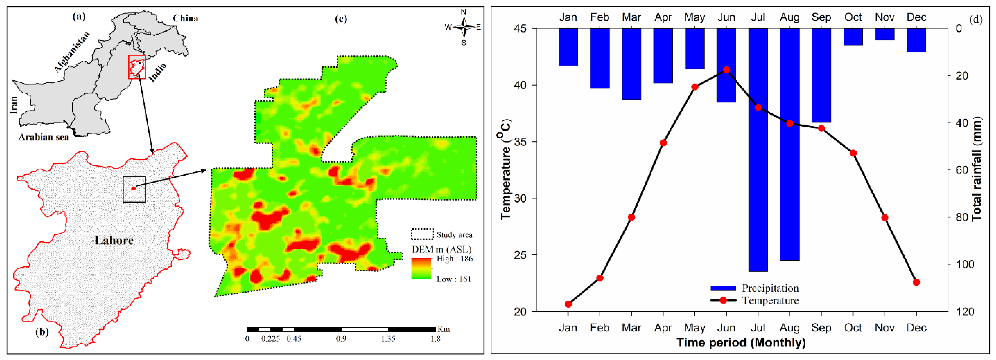
2.1. Study Area

This study focuses on a typical community within the city of Lahore, located in the southern Punjab province of Pakistan, as shown in Figure 1c. The geographic coordinates are 73°–74° east longitude and 30°–31.5° north latitude, with an average elevation of 172 m above sea level. The study area covers 2.71 km². Land use within the community is primarily residential, with interspersed commercial and recreational areas. This composition offers a representative sample of urban hydrological and environmental dynamics within the broader perspective of Lahore and the Punjab region.

Lahore experiences distinct seasonal weather patterns (Figure 1d). The average annual precipitation is 628.8 mm, with the majority concentrated in the monsoon season (July to September). The average monthly rainfall during this period is 52.4 mm. These pronounced seasonal variations in temperature and precipitation significantly influence hydrological dynamics, water resource availability, and urban environmental conditions within the city.

2.2. Data Collection

A comprehensive understanding of drainage system performance necessitates a diverse array of datasets. This study gathered data from several sources, as shown in

Table 1. Sources of data acquisition.

S. No	Data Type	Period	Source
1	Rainfall data (hourly)	2001–2020	PMD
2	Sub-catchments, links, and junction	2021	NHA
3	DEM (12.5 m × 12.5 m)		https://search.asf.alaska.edu/#/ (accessed on 15 October 2022)

. The Pakistan Meteorological Department (PMD) provided 20 years (2001–2020) of hourly rainfall data, providing insights into historical patterns and system capacity impacts. The National Highway Authority (NHA) provided the drainage system’s physical structure data, encompassing sub-catchments, links, and junctions, as shown in Table 1. These data are vital for modeling flow dynamics and identifying system vulnerabilities. To ensure accurate terrain representation and hydrological parameter calculations (e.g., slope and flow accumulation), a high-resolution (12.5-m pixel size) digital elevation model (DEM) was obtained from the Alaska Satellite Facility (ASF).

2.3. Data Integration and Preparation

The data from these diverse sources were integrated and formatted for compatibility using ArcGIS 10.7. This dataset fell into two main categories: spatial data (geospatial information like AutoCAD drawings and the DEM) and non-spatial data (urban drainage system attributes from the NHA). The database encompasses 74 sub-catchments, 77 links, and 78 junctions, covering 2.71 km². The AutoCAD file was converted to an ArcMap shapefile, and the entire dataset was then formatted as SWMM input data to enable simulations for assessing the existing drainage system.

2.4. Model Selection

This study utilizes the stormwater management model (SWMM), version 5.2 (released February 2022), developed by the United States Environmental Protection Agency (first introduced in 1971). SWMM is a dynamic rainfall-runoff model that is capable of simulating both single-event and continuous long-term scenarios. It is widely used in stormwater runoff analysis, drainage system design, and performance evaluation [36,37,38].

SWMM aligns with local, state, and national stormwater management goals, specifically targeting runoff volume reduction through infiltration and retention and minimizing pollutant discharge to waterbodies [39]. It is designed for urban areas where impervious surfaces and drainage systems significantly modify natural hydrology [39]. SWMM has a proven track record of successful applications worldwide, demonstrating its value in addressing urban water quality and quantity challenges [38,39,40,41,42,43,44].

2.5. Model Development

2.5.1. Model Input Parameters

The key components of SWMM include rain gauges, sub-catchments, junctions, outfalls, storage units, flow dividers, conduits, orifices, pumps, weirs, and outlets. Table S1 outlines the essential input data required by SWMM. A rain gauge (R1) was strategically placed within the study area and linked to sub-catchments to provide rainfall intensity data for the SWMM model. GIS was employed to determine sub-catchment areas, conduit lengths, and node invert elevations from existing data sources. Sub-catchment shapes were digitized based on a terrain analysis using Google Earth and ArcGIS. A DEM was extracted from the sub-catchment shapefile, and its attribute table was used to compute the cell counts for each sub-catchment. The area was then calculated using Equation (1):

$$A=R_n\times S^2$$

(1)

where A is the area, $R_n$ is number of raster cells, and S is DEM cell size. Using ArcGIS, the width, imperviousness, slope, and roughness were calculated for each sub-catchment. Precise catchment areas were determined using the ArcGIS field calculator and provided as SWMM model input. Slope (0–102%) and roughness (0.11–0.89) maps were derived using ArcGIS and the ALOS PALSAR DEM (12.5 × 12.5 m resolution), as shown in Figure 2.

A GIS spatial analysis was used to compute the roughness coefficient, quantifying surface resistance to water flow and aligning with Manning’s ‘n’ in SWMM [40]. This involved calculating the mean, maximum, and minimum focal statistical (FA) layers (Neighborhood tool) and using the Raster calculator (Map Algebra tool) using Equation (2) [45].

$$RG=\frac{{FS}_{mean}-{FS}_{min}}{{FS}_{max}-{FS}_{min}}$$

(2)

Other parameters like depression storage, or the capacity of a surface to retain water before runoff, were incorporated with values assigned according to the SWMM user manual. This included factoring in the percentage of impervious areas without depression storage [39,40], initially set at a SWMM default value of 25%.

SWMM offers various computational methods for infiltration (Horton, Green–Ampt, modified Green–Ampt, SCS curve number). The modified Green–Ampt method was selected due to its suitability for rainfall intensities exceeding the soil infiltration capacity. The key parameters for this method include initial the moisture deficit, saturated hydraulic conductivity, and soil suction head [46]. For flow routing, the kinematic wave method was chosen, as it allows for spatiotemporal flow variations within conduits [40]. This provides an accurate, efficient choice for long-term simulations where dynamic flow is not expected to impact the model outcomes significantly.

2.5.2. Sensitivity Analysis of Model Input Parameters

A sensitivity analysis is a vital step in SWMM model calibration. It helped determine the model’s output response to changes in individual input parameters. This process identified the most influential parameters and optimized their values during calibration. Previous studies investigated the sensitivity of parameters such as the slope, width, percentage of impervious surfaces without depression storage, percent imperviousness, manning’s roughness coefficient, infiltration parameters, and depression storage [27,47,48,49].

This study conducted a pre-calibration sensitivity analysis to determine the parameters with the greatest impact on the model’s behavior. Each parameter was individually varied within 50% of its initial value while holding the others constant. The relative sensitivity (S) was calculated using Equation (3) [50]:

$$S=\frac{\partial \mathrm{R}}{\partial \mathrm{P}}\times \frac{P}{R}$$

(3)

where S is parameter sensitivity, ∂R represents the difference between the original model output and the new model output, ∂P represents the difference between the original parameter value and the adjusted parameter value, R represents the actual model output, and P represents the original value of a parameter [51].

The evaluated parameters included Manning’s roughness coefficient, saturated hydraulic conductivity, Green–Ampt infiltration parameters, and the initial soil moisture [51].

Table 2. Sensitivity analysis of the SWMM model parameters.

Parameter	Initial Value	Calibrated Value/Range (For Each Sub-Catchment)	Source of Data
Area of sub-catchments (ha)	GIS-calculated	Original value	GIS-calculated
Width	GIS-calculated	Original value	GIS-calculated
Slope (%)	0.5	0.11–1.5	[38]
% Impervious	50	0.4–11.104	[38]
N-imperv.	0.01	0.01	[38]
N-perv.	0.10	0.1	[38]
Dstore-imperv (mm)	0.05	0.05	[38]
Dstore-perv (mm)	0.05	10.5	[38]
% Zero-imperv	50	25	[38]
Infiltration model (modified Green–Ampt)
Suction head (mm)	3.5	20	[38,52]
Conductivity (mm/h)	0.5	10	[38,52]
Initial soil moisture Deficit (fraction)	0.26	0.5	[38,52]

summarizes the parameters, their original values, and their final calibrated values.

2.5.3. Model Calibration and Validation

Model calibration is crucial to ensure the model’s ability to accurately represent real-world conditions. This process involves adjusting model parameters iteratively to optimize the agreement between the simulated results and the observed water depth and volume values within the stormwater system [53,54]. Since this study focuses on model performance assessment rather than direct modification of the existing system (Figure S1), calibration acts as a key performance indicator.

Model performance is typically evaluated using the root mean square error (RMSE) and Nash–Sutcliffe efficiency (NSE) [55]. A lower RMSE indicates better performance, with zero signifying perfect accuracy [56]. NSE ranges from −∞ to 1, with values closer to 1 suggesting superior model efficiency [57]. An NSE value of NSE ≥ 0.5 often indicates good model performance [58]. However, it is important to interpret RMSE and NSE in detail and recognize essential modeling uncertainties in hydrological modeling [59].

This study calibration process utilizes event-based rainfall and discharge data, as shown in Table S2 and Table 3. Initial comparisons between the observed data and SWMM simulations are visualized, as shown in Figure 5. Model validation involves comparing the simulated and observed data using goodness-of-fit criteria [60], which are explained in detail in the Supplementary Materials.

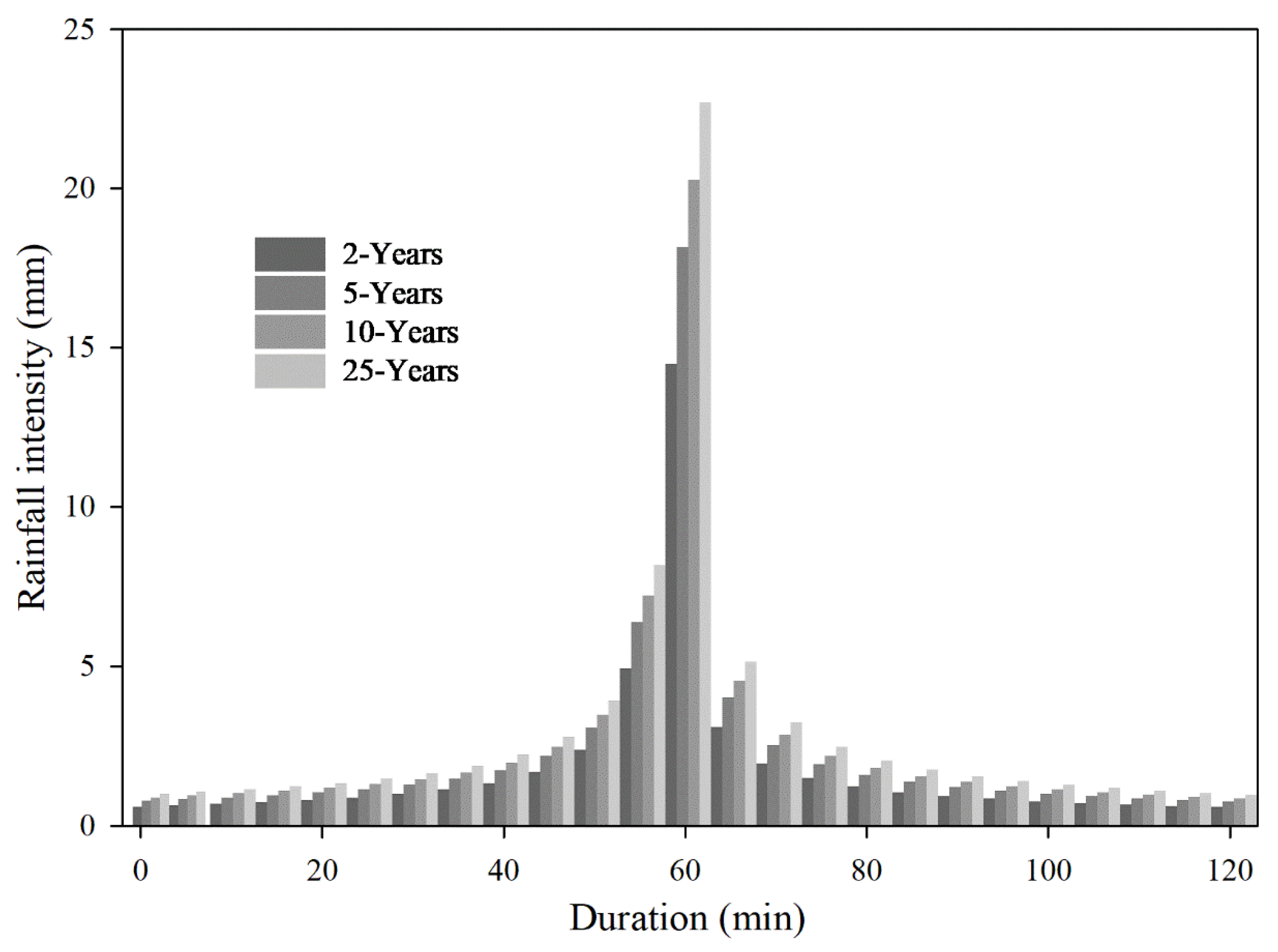
2.6. Estimation of Hyetograph

2.6.1. Analysis of Rainfall Data

Rainfall data analysis began with a rainfall frequency analysis utilizing historical hourly precipitation data. The annual maximum rainfall values were extracted from the dataset and ranked from largest to smallest (Table S3). The rank-order (M) method was used for ordering and plotting the rainfall data from the largest value (rank 1) to the smallest (rank n). To determine the return period, which reflects the probability of a specific rainfall event being equaled or exceeded in any given year, the Weibull plotting position equation (Equation (4)) was employed:

$$T=\frac{(y+1)}{M}$$

(4)

where T is the return period in years, y is the number of years of data, and M is the rank of the data in the time series.

2.6.2. Log-Pearson Type III Distribution

This study employed the widely recognized LPT-III distribution to analyze the probability distribution of rainfall events [61,62,63]. LPT-III uses a logarithmic transformation to calculate rainfall intensity for various durations and return periods [64]. We analyzed the maximum annual rainfall events using LPT-III to determine the return period values for the available dataset. The suitability of LPT-III for rainfall design analysis has been demonstrated in a recent comparison study by Mudashiru et al. [65], where it outperformed methods such as Normal, Gumbel, Pearson III, and Log-normal distributions. Our own findings confirm the appropriateness of LPT-III for this analysis. Computational expressions for rainfall intensity determination using the LPT-III distribution are provided in the Supplementary Materials in Tables S3 and S4.

2.6.3. Generation of Shorter-Duration Events

The rainfall depths were analyzed according to durations shorter than their full duration (24 h). Many researchers have used the empirical reduction formula in Equation (5) to calculate rainfall depths for durations less than 24 h [66]. Equation (5) was given the best estimation of short-duration rainfall for 120 min to obtain the intensity duration frequency (IDF) curve, as shown in Figure 3.

$$R_t=R_{24}(\frac{T_d}{24}{)}^{\frac{1}{3}}$$

(5)

Here, R_t is the maximum hourly rainfall depth for duration t, R₂₄ is the maximum daily rainfall depth, and T_d is the time duration in hours. After obtaining the rainfall depth as shown in Figure 3a, the rainfall intensity presented in Figure 3b was calculated using Equation (6):

$$I_t=\frac{P_t}{T_d}$$

(6)

where I_t = rainfall intensity, P_t= rainfall depth, and T_d = duration.

2.6.4. Alternating Block Method

This study employed the ABM to generate a synthetic hyetograph for flood analysis utilizing an IDF curve (Figure 3). The ABM ensures that the accumulated rainfall depth at the storm center aligns precisely with the depth obtained from the IDF curve for that specific duration (Equation (6)). The design storm exhibits peak intensity at its center, corresponding to the rainfall intensity obtained from the IDF curve.

The steps followed for generating a synthetic hyetograph include the following. First, after selecting a design return period, rainfall depths were obtained from the IDF curve for increasing durations (Δt, 2Δt, 3Δt, etc.) up to the design storm duration (T_d) (Equation (6)). Then, the differences between consecutive rainfall depth values were calculated to determine rainfall increments for each time interval (Δt). Finally, these increments were arranged with the highest intensity at the center. The remaining blocks were placed in descending order, alternating before and after the center block, forming the hyetograph design, as shown in Figure 4. This approach is based on established methods by Chow et al. [46], as shown in Equation (7):

$$T_d=t_n\ast \Delta \mathrm{t}$$

(7)

where $T_d$ is the duration, and $t_n$ is the total number of time intervals of duration Δt.

The study area lacked predefined storm patterns for hyetograph design. Unlike methods like the Chicago design storm, which relies on historical storm patterns, the ABM offers flexibility in analyzing rainfall intensity and duration from existing data and creating potential storm profiles. This flexibility is essential for areas with diverse rainfall events.

The ABM is complemented by the LPT-III distribution. LPT-III handles the skewed nature of rainfall data and aids in predicting extreme rainfall events based on exiting data. The combination of ABM and LPT-III enables a dynamic and data-driven approach to rainfall pattern prediction and stormwater system design, especially in areas lacking typical storm profiles. This tailored approach ensures that hydrological analyses and designs reflect the true characteristics of local rainfall events, enhancing their overall reliability and effectiveness.

2.7. Spatial Distribution of Flood Risk in Sub-Catchments

The flood risk density map was generated by floods occurring during the SWMM simulation in the nodes by using GIS along with the Kernel density function and reclassifying it according to the severity of the risk. It is common practice to conduct mapping projects to pinpoint risk areas, such as those with a high frequency of floods [67]. Caradot et al. [68] recommend using the Kernel density function to show the spatial distribution of flood risk. The Kernel risk density, represented as KRD, is computed for every individual point (also known as a pixel) inside the study area. Equation (8) was used to calculate the flood risk map density for the flooding in the current drainage system.

$$FRD=\frac{{\sum }_{i=1}^n(Xi, Yi)}{S}$$

(8)

In Equation (8), $FRD$ represents the flood risk density, and ${\sum }_{i=1}^n(Xi, Yi)$ denotes the summation of the coordinates (Xi, Yi) of each individual point (i) within the study area, where Yi is a decreasing smoothing coefficient and S is the area of a circle with radius R that contains n junction flooding events, as shown in Equations (9) and (10). The value of Xi value corresponds to the risk score for junction flooding i, or the number of events observed for each map pixel. n is the total number of data points (also known as pixels) within the study area where flood risk data were analyzed.

$$Y_i=\left(1-{\left(\frac{r_i}{R}\right)}^2\right) if r_i<R$$

(9)

$$Y_i=0 if r_i>R$$

(10)

In Equations (9) and (10), “ri” represents the distance between the pixel and the flooding point “i”.

3. Results

3.1. Model Calibration and Validation

Before utilizing the SWMM model for result-oriented simulations, a rigorous calibration process is essential to represent runoff at a pre-defined junction accurately [69,70]. Statistical analyses such as NSE, RMSE, and R² are the standard tools for evaluating model consistency and validating its suitability for further analysis [71,72].

This study utilized SWMM to analyze and predict stormwater runoff. A rigorous calibration and validation process was conducted based on four historical rainfall events with low and high rainfall intensities to ensure the model accuracy and reliability. This study employed a rigorous SWMM calibration and validation process using four historical rainfall events representing low and high intensities. In Figure 5a,b, two events (low rainfall: 3 July 2018; high rainfall: 20 August 2020), as shown in Table S1, were used for calibration. The model parameters were iteratively adjusted to achieve a strong agreement between the simulated and observed runoff data. This establishes the model’s ability to reproduce runoff under diverse rainfall conditions. In Figure 5c,d, the remaining two events (low rainfall: 13 August 2020; high rainfall: 21 July 2022), as shown in Table S2, were used for validation. This was used to assess the calibrated model’s ability to predict runoff without further parameter adjustments, demonstrating its robustness and ability to generalize to unseen events.

Including both low and high rainfall events ensures that the SWMM model is effective across a range of hydrological conditions. NSE, RMSE, and R² were calculated using rainfall and discharge data from the four events, as shown in Figure 5. The measured discharge ranged from 0.63 to 1.10 cubic feet per second (CFS), while the simulated discharge ranged from 0.48 to 0.81 CFS, as indicated in Table 3. The NSE values (0.71–0.78) indicated good model efficiency. The RMSE values (0.28–0.44) were reasonable, especially for rainfall-runoff modeling. The R² values (0.84–0.89) demonstrated a strong correlation between the observed and simulated data across events.

Table 3. SWMM model validation data (NSE, RMSE, and R²) based on observed and simulated runoff.

		Model Calibration				Model Validation
		Event 1		Event 2		Event 3		Event 4
Statistical analysis		Obs	Sim	Obs	Sim	Obs	Sim	Obs	Sim
	Average inflow (CFS)	0.63	0.48	0.88	0.64	0.60	0.50	1.10	0.81
Evaluation statistics	NSE	0.72		0.76		0.71		0.78
	RMSE	0.43		0.44		0.28		0.41
	R2	0.85		0.86		0.84		0.89

Note(s): Obs = observed, Sim = simulation.

Table 3. SWMM model validation data (NSE, RMSE, and R²) based on observed and simulated runoff.

		Model Calibration				Model Validation
		Event 1		Event 2		Event 3		Event 4
Statistical analysis		Obs	Sim	Obs	Sim	Obs	Sim	Obs	Sim
	Average inflow (CFS)	0.63	0.48	0.88	0.64	0.60	0.50	1.10	0.81
Evaluation statistics	NSE	0.72		0.76		0.71		0.78
	RMSE	0.43		0.44		0.28		0.41
	R2	0.85		0.86		0.84		0.89

Note(s): Obs = observed, Sim = simulation.

3.2. Assessment of the Current Drainage System

SWMM simulations were used to evaluate the existing drainage system’s performance under current (2022) land-use conditions and for four different return periods. The results indicate that a significant portion of rainfall within the study area is converted to surface runoff. For a 2-year return period rainfall (75.44 mm), the estimated peak runoff is 0.18 m³/s, as shown in

Table 4. Performance of the current drainage system based on a design rainfall event.

Design Storm (Years)	2 Years	5 Years	10 Years	25 Years
Total rainfall (mm/hr)	75.44	97.46	110.11	124.51
Peak runoff (m³/s)	0.18	0.24	0.27	0.31
Total outfall volume (gal/s)	8.16	24.21	31.53	41.06
Number of flooded nodes	64	64	64	65

.

Frequent flooding occurred at the junctions, even under the 2-year return period, as shown in Figure 6a, indicating that the drainage system may have an inadequate capacity to handle heavy rainfall events. Flooding was observed in both central and upstream junctions, as shown in Figure 6b. Based on the SWMM model simulation, Figure 6c classifies the flood severity for the current drainage system under different return periods. The flood severity was classified using a geometric interval approach for consistency, which signifies severe flooding that poses risks to public safety and drainage infrastructure.

At the 2-year return period, only 0.3% of the area experienced no flooding, while 4.0% and 8.5% experienced medium and high flooding, respectively (Figure 6c). This trend intensified at longer return periods, with the 25-year event showing 0.2% NF and 13.7% VHF. While inadequate design may contribute to flooding, it is important to acknowledge the complex nature of urban hydrology and potential changes in rainfall patterns since the system’s installation (originally designed for a 2-year return period). As the system is relatively new, the focus shifts towards adaptation strategies rather than comprehensive replacement. These results suggest that the current drainage system may not sufficiently handle increasingly intense rainfall events. Management strategies like LID practices are needed to mitigate future flood risks. Implementing LID practices is recommended to address existing flooding issues. LID practices aim to control runoff at its source, thereby enhancing drainage system capacity.

3.3. Flood Risk Density

Figure 7 spatially represents flood risk density based on a simulated design rainfall event. Flooding occurred at numerous junctions throughout the study area during the simulation, as shown in Figure 6b. Flood risk is classified as very low, low, moderate, high, or very high, with corresponding percentages of the affected area for different return periods, as shown in Figure 7. The spatial distribution of flood risk indicates low and very low probabilities in the western, northwestern, and southwestern borders. Moderate flood risk covers the largest portion of the study area. High and very high flood risk zones are primarily located in the lower and upper regions.

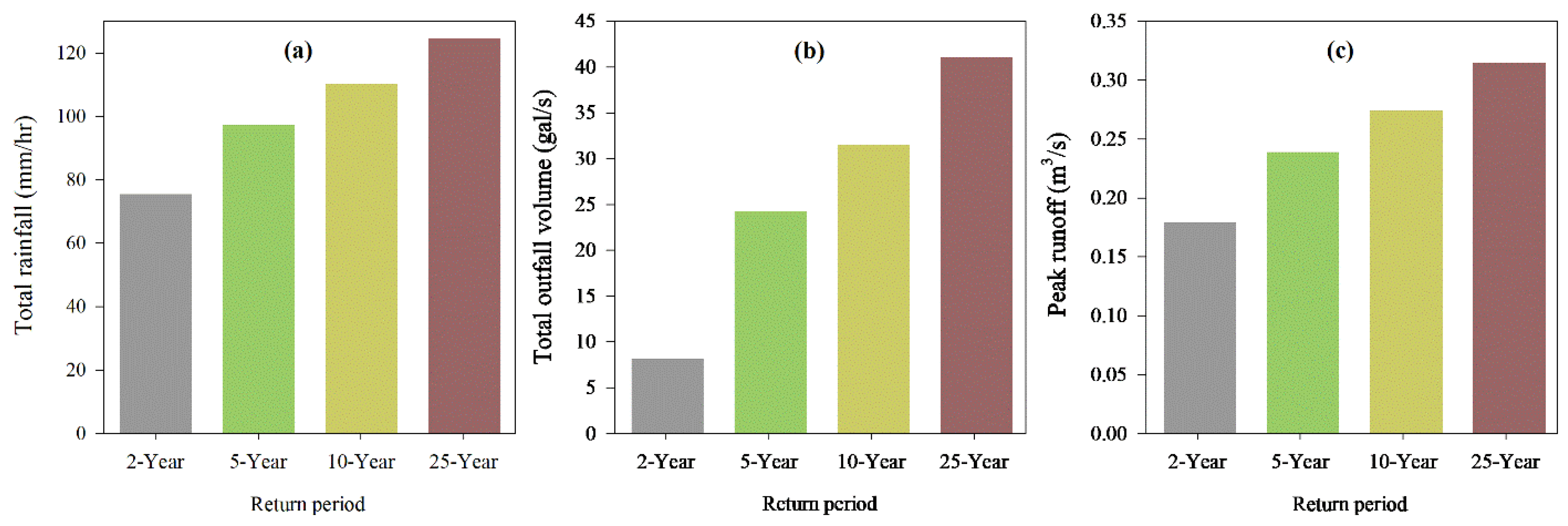
3.4. Assessment Based on Design Rainfall Events

Four design storms with return periods (2, 5, 10, and 25 years) were simulated using the SWMM to evaluate the existing drainage system’s performance under various rainfall scenarios. Figure 8 visualizes the relationship between total rainfall, peak runoff, and total outfall volume. The results in Table 4 reveal that a significant portion of rainfall within the study area is converted to surface runoff, posing a challenge for the drainage system, especially during high-intensity events.

A detailed analysis in Table 4 highlights that the total rainfall depth increases with longer return periods, ranging from 75.44 mm/h (2-year) to 124.51 mm/h (25-year). Peak runoff discharge also increases proportionally, rising from 0.18 m³/s (2-year) to 0.31 m³/s (25-year). This suggests a reduced capacity to convey peak flows as storm intensity and volume increase. The total outfall volume, the cumulative outflow, significantly increases from 8.16 gal/s (2-year) to 41.06 gal/s (25-year), emphasizing the potential for severe inundation and flooding risks during major storms. Interestingly, the number of flooded nodes remains relatively constant across all the simulated return periods from 64 to 65. This indicates potential limitations in the existing drainage system’s capacity to prevent localized flooding, even during minor rainfall events.

3.5. Total Flooded Volume and Area Based on Different Design Rainfall Event Conditions

Table 5. Total flood volume and total flooding area at different return periods.

	Design Rainfall Event (2 h) Simulation
Return Period	Total Flood Volume (106 gal)	Total Flooding Area (%)	Total Area (km2)
2 years	0.07	59.86	2.71
5 years	0.09	78.22
10 years	0.10	88.69
25 years	0.11	99.94

reveals the results of 2 h event-based simulations for various return periods, highlighting the total flood volume and the extent of the flooded area. Return periods represent the probability of a specific rainfall event occurring. For example, a 2-year return period storm produced 0.07 million gallons (10⁶ gal) of total flood volume, inundating approximately 60% of the study area. As the return period increases, the flood volume and the percentage of the flooded area increase dramatically, as shown in Figure 9. At a 25-year return period, the total flood volume reaches 0.11 (10⁶ gal), and nearly the entire region (99.94%) is flooded.

These findings demonstrate the current drainage system’s inadequacy. Significant flooding occurred, even during relatively minor 2-year return period events, and the situation worsened considerably at longer return periods. This suggests that the system may not have been designed to accommodate the increased rainfall intensity associated with potential climate change effects. Urgent infrastructure upgrades are necessary to enhance the system’s capacity to manage the increasing intensity and volume of storm events. A comprehensive re-evaluation of the current system, followed by the implementation of resilient and adaptive stormwater management solutions (like LID practices), is crucial to mitigate future flood risks.

4. Discussion

This study highlights the critical need to re-evaluate and upgrade urban drainage systems in rapidly developing regions facing increased flood risks due to urbanization and climate change [1,2]. The model calibration and validation results demonstrate the suitability of SWMM for simulating runoff and assessing drainage system performance [69,70]. While the NSE and R² values indicate acceptable model performance, the RMSE scores reveal potential areas for further refinement. The findings of good model efficiency (NSE: 0.71–0.78) and a strong correlation between the observed and simulated data (R²: 0.84–0.89) during SWMM model calibration and validation highlight the importance of these rigorous processes for accurate flood risk assessments. The results confirm the working hypothesis that the existing drainage system in our study area is likely inadequate. Frequent flooding, even during relatively minor events, highlights the challenges posed by evolving rainfall patterns influenced by climate change and the complex interaction between urbanization and infrastructure design [6,7]. A spatial analysis identifies specific flood-prone zones, suggesting that targeted mitigation strategies are needed [8]. The consistent number of flooded nodes across varying return periods raises concerns about the drainage system’s limited capacity to prevent localized flooding risk.

While inadequate infrastructure design plays a role, a broader perspective is essential to address these challenges [4,5]. The dynamic nature of urban hydrology and the potential impacts of climate change on rainfall patterns must be considered [7,8,73]. As the system is relatively new, a comprehensive focus on adaptation and resilience becomes crucial, emphasizing strategies like LID practices [26,27]. Implementing LID practices offers a promising solution for decentralized, nature-based stormwater management, reducing pressure on existing infrastructure and enhancing overall resilience [21,74].

These study findings are supported by previous research investigating the limitations of traditional drainage systems in the face of climate change [25]. Our methodology, integrating SWMM simulations, the LPT-III distribution, the ABM, and GIS spatial analysis offers a robust framework for identifying flood-prone areas and quantifying risks [19,20,26,27]. The use of LPT-III ensures that the analysis accurately reflects the skewed nature of extreme precipitation events, which is crucial for data-scarce regions.

This study recommends proactive measures to address flood risks and enhance Lahore drainage system resilience. Firstly, expanding and upgrading existing infrastructure is crucial to accommodate higher runoff volumes, as highlighted in previous studies [22,23]. Additionally, integrating citywide low-impact development (LID) practices is essential. These practices, including bioretention cells, green roofs, infiltration trenches, permeable pavements, rain barrels or cisterns, rooftop disconnections, and vegetative swales, promote infiltration, reduce runoff, and improve water quality [21]. Updating design standards to align with projected climate change impacts is imperative to ensure new infrastructure can withstand increasingly intense rainfall events [25]. Furthermore, prioritizing data collection on rainfall patterns, geospatial information, and flood monitoring is crucial for effective risk assessments and mitigation planning [20]. Lastly, community engagement is vital for raising flood risk awareness and fostering long-term success in mitigation efforts, emphasizing the importance of resident involvement [24].

5. Conclusions

This study reveals the critical limitations of Lahore’s current urban drainage system and emphasizes the urgent need for adaptation in the face of climate change and urbanization. The existing drainage infrastructure, designed for a 2-year return period, cannot adequately handle the increased rainfall intensity and volume observed in our analysis. The results indicate frequent flooding, even during relatively moderate storm events. The methodology employed integrating SWMM simulations, the LPT-III distribution, the ABM, and GIS spatial analysis provides a robust framework for flood risk assessment in data-scarce regions.

References

1. Parkinson, J. Urban drainage in developing countries—Challenges and opportunities. WATERLINES 2002, 20, 2–5. [Google Scholar] [CrossRef]
2. Xu, Z.; Xu, J.; Yin, H.; Jin, W.; Li, H.; He, Z. Urban river pollution control in developing countries. Nat. Sustain. 2019, 2, 158–160. [Google Scholar] [CrossRef]
3. Zhang, H.; Yang, Z.; Cai, Y.; Qiu, J.; Huang, B. Impacts of Climate Change on Urban Drainage Systems by Future Short-Duration Design Rainstorms. Water 2021, 13, 2718. [Google Scholar] [CrossRef]
4. Yadav, B.; Gupta, P.K.; Patidar, N.; Himanshu, S.K. Ensemble modelling framework for groundwater level prediction in urban areas of India. Sci. Total Environ. 2020, 712, 135539. [Google Scholar] [CrossRef] [PubMed]
5. Anees, M.; Sajjad, S.; Joshi, P.K. Characterizing urban area dynamics in historic city of Kurukshetra, India, using remote sensing and spatial metric tools. Geocarto Int. 2019, 34, 1584–1607. [Google Scholar] [CrossRef]
6. Vemula, S.; Raju, K.S.; Veena, S.S.; Kumar, A.S. Urban floods in Hyderabad, India, under present and future rainfall scenarios: A case study. Nat. Hazards 2019, 95, 637–655. [Google Scholar] [CrossRef]
7. Bisht, S.; Chatterjee, C.; Kalakoti, S.; Upadhyay, P.; Sahoo, M.; Panda, A. Modeling urban floods and drainage using SWMM and MIKE URBAN: A case study. Nat. Hazards 2016, 84, 749–776. [Google Scholar] [CrossRef]
8. Paul, S.; Ghosh, S.; Mathew, M.; Devanand, A.; Karmakar, S.; Niyogi, D. Increased Spatial Variability and Intensification of Extreme Monsoon Rainfall due to Urbanization. Sci. Rep. 2018, 8, 3918. [Google Scholar] [CrossRef] [PubMed]
9. Chan, S.C.; Kendon, E.J.; Fowler, H.J.; Youngman, B.D.; Dale, M.; Short, C. New extreme rainfall projections for improved climate resilience of urban drainage systems. Clim. Serv. 2023, 30, 100375. [Google Scholar] [CrossRef]
10. D’Ambrosio, R.; Longobardi, A.; Schmalz, B. SuDS as a climate change adaptation strategy: Scenario-based analysis for an urban catchment in northern Italy. Urban. Clim. 2023, 51, 101596. [Google Scholar] [CrossRef]
11. Ji, X.; Dong, W.; Wang, W.; Dai, X.; Huang, H. Impacts of Climate Change on Extreme Precipitation Events and Urban Waterlogging: A Case Study of Beijing. Nat. Hazards Rev. 2024, 25, 05023014. [Google Scholar] [CrossRef]
12. Ahmad, M.N.; Shao, Z.; Javed, A. Mapping impervious surface area increase and urban pluvial flooding using Sentinel Application Platform (SNAP) and remote sensing data. Environ. Sci. Pollut. Res. 2023, 30, 125774–125789. [Google Scholar] [CrossRef] [PubMed]
13. Chan, F.K.S.; Wang, Z.; Chen, J.; Lu, X.; Nafea, T.; Montz, B.; Adekola, O.; Pezzoli, A.; Griffiths, J.; Peng, Y.; et al. Selected global flood preparation and response lessons: Implications for more resilient Chinese Cities. Nat. Hazards 2023, 118, 1767–1796. [Google Scholar] [CrossRef]
14. Idowu, D.; Zhou, W. Global Megacities and Frequent Floods: Correlation between Urban Expansion Patterns and Urban Flood Hazards. Sustainability 2023, 15, 2514. [Google Scholar] [CrossRef]
15. Xu, T.; Xie, Z.; Jiang, F.; Yang, S.; Deng, Z.; Zhao, L.; Wen, G.; Du, Q. Urban flooding resilience evaluation with coupled rainfall and flooding models: A small area in Kunming City, China as an example. Water Sci. Technol. 2023, 87, 2820–2839. [Google Scholar] [CrossRef]
16. Zhong, C.; Guo, H.; Swan, I.; Gao, P.; Yao, Q.; Li, H. Evaluating trends, profits, and risks of global cities in recent urban expansion for advancing sustainable development. Habitat Int. 2023, 138, 102869. [Google Scholar] [CrossRef]
17. Balbastre-Soldevila, R.; García-Bartual, R.; Andrés-Doménech, I. A Comparison of Design Storms for Urban Drainage System Applications. Water 2019, 11, 757. [Google Scholar] [CrossRef]
18. Salinas-Rodriguez, C.; Gersonius, B.; Zevenbergen, C.; Serrano, D.; Ashley, R. A Semi Risk-Based Approach for Managing Urban Drainage Systems under Extreme Rainfall. Water 2018, 10, 384. [Google Scholar] [CrossRef]
19. Zhu, Z.; Chen, Z.; Chen, X.; He, P. Approach for evaluating inundation risks in urban drainage systems. Sci. Total Environ. 2016, 553, 1–12. [Google Scholar] [CrossRef] [PubMed]
20. Zhou, Q.; Leng, G.; Su, J.; Ren, Y. Comparison of urbanization and climate change impacts on urban flood volumes: Importance of urban planning and drainage adaptation. Sci. Total Environ. 2019, 658, 24–33. [Google Scholar] [CrossRef] [PubMed]
21. Guptha, G.C.; Swain, S.; Al-Ansari, N.; Taloor, A.K.; Dayal, D. Evaluation of an urban drainage system and its resilience using remote sensing and GIS. Remote Sens. Appl. Soc. Environ. 2021, 23, 100601. [Google Scholar] [CrossRef]
22. Adugna, D.; Lemma, B.; Jensen, M.B.; Gebrie, G.S. Evaluating the hydraulic capacity of existing drain systems and the management challenges of stormwater in Addis Ababa, Ethiopia. J. Hydrol. Reg. Stud. 2019, 25, 100626. [Google Scholar] [CrossRef]
23. Bulti, T.; Abebe, B.G. Analyzing the impacts of urbanization on runoff characteristics in Adama city, Ethiopia. SN Appl. Sci. 2020, 2, 1151. [Google Scholar] [CrossRef]
24. Sambeto, B.; Reddythta, D.; Kebebew, A.S. Assessment of the drainage systems performance in response to future scenarios and flood mitigation measures using stormwater management model. City Environ. Interact. 2023, 19, 100111. [Google Scholar] [CrossRef]
25. Miller, J.D.; Hutchins, M. The impacts of urbanisation and climate change on urban flooding and urban water quality: A review of the evidence concerning the United Kingdom. J. Hydrol. Reg. Stud. 2017, 12, 345–362. [Google Scholar] [CrossRef]
26. Akter, A.; Tanim, A.H. Estimating urban flood hazard zones using SWMM in Chittagong City. Tech. J. River Res. Inst. 2016, 13, 87–101. [Google Scholar]
27. Jiang, L.; Chen, Y.; Wang, H. Urban flood simulation based on the SWMM model. Proc. Int. Assoc. Hydrol. Sci. 2015, 368, 186–191. [Google Scholar] [CrossRef]
28. Shao, Z.; Ahmad, M.N.; Javed, A.; Islam, F.; Jahangir, Z.; Ahmad, I. Expansion of Urban Impervious Surfaces in Lahore (1993–2022) Based on Gee and Remote Sensing Data. Photogramm. Eng. Remote Sens. 2023, 89, 479–486. [Google Scholar] [CrossRef]
29. Shrestha, B.Z. A Fusion of Remotely Sensed Data to Map the Impervious Surfaces of Growing Cities of Punjab, Pakistan. Master Dissertation, University of Nevada, Las Vegas, NV, USA, 2021. [Google Scholar]
30. Rana, I.A.; Asim, M.; Aslam, A.B.; Jamshed, A. Disaster management cycle and its application for flood risk reduction in urban areas of Pakistan. Urban. Clim. 2021, 38, 100893. [Google Scholar] [CrossRef]
31. Liu, S.; Wang, Y.; Zhang, G.J.; Gong, P.; Wei, L.Y.; He, Y.J.; Li, L.J.; Wang, B. Effects of Urbanization in China on the East Asian Summer Monsoon as Revealed by Two Global Climate Models. J. Geophys. Res.-Atmos. 2024, 129, e2023JD039737. [Google Scholar] [CrossRef]
32. Omer, S. Lahore’s Population Witnesses Steady Annual Growth of Three Percent. 18 October 2023. Available online: https://www.pakistantoday.com.pk/2023/05/16/lahores-population-witnesses-steady-annual-growth-of-three-percent/ (accessed on 18 October 2023).
33. Zia, S.; Nasar-u-Minallah, M.; Zahra, N.; Hanif, A. The Effect of Urban Green Spaces in Reducing Urban Flooding in Lahore, Pakistan, Using Geospatial Techniques. Geogr. Environ. Sustain. 2022, 15, 47–55. [Google Scholar] [CrossRef]
34. Wahl, T.; Jain, S.; Bender, J.; Meyers, S.D.; Luther, M.E. Increasing risk of compound flooding from storm surge and rainfall for major US cities. Nat. Clim. Chang. 2015, 5, 1093–1097. [Google Scholar] [CrossRef]
35. Yin, H.; Zheng, F.; Duan, H.-F.; Savic, D.; Kapelan, Z. Estimating Rainfall Intensity Using an Image-Based Deep Learning Model. Engineering 2023, 21, 162–174. [Google Scholar] [CrossRef]
36. Johannessen, G.; Hamouz, V.; Gragne, A.S.; Muthanna, T.M. The transferability of SWMM model parameters between green roofs with similar build-up. J. Clean. Prod. 2019, 569, 816–828. [Google Scholar] [CrossRef]
37. Tuomela, C.; Sillanpää, N.; Koivusalo, H. Assessment of stormwater pollutant loads and source area contributions with storm water management model (SWMM). J. Environ. Manag. 2019, 233, 719–727. [Google Scholar] [CrossRef] [PubMed]
38. Rossman, L.A.; Michelle, S.A. Storm Water Management Model User’s Manual, Version 5.2; National Risk Management Research Laboratory, Office of Research and Development, US Environmental Protection Agency: Washington, DC, USA, 2022.
39. Rossman, L.A.; Huber, W.C. Storm Water Management Model Reference Manual Volume I–Hydrology; U.S. EPA Office of Research and Development: Washington, DC, USA, 2016.
40. James, W.; Rossman, L.A.; James, W.R.C. User’s Guide to SWMM 5: [Based on Original USEPA SWMM Documentation], 13th ed.; CHI: Guelph, ON, Canada, 2010. [Google Scholar]
41. Randall, M.; Sun, F.; Zhang, Y.; Jensen, M.B. Evaluating Sponge City volume capture ratio at the catchment scale using SWMM. J. Environ. Manag. 2019, 246, 745–757. [Google Scholar] [CrossRef] [PubMed]
42. Xu, T.; Jia, H.; Wang, Z.; Mao, X.; Xu, C. SWMM-based methodology for block-scale LID-BMPs planning based on site-scale multi-objective optimization: A case study in Tianjin. Front. Environ. Sci. Eng. 2017, 11, 1. [Google Scholar] [CrossRef]
43. Jia, H.; Liu, Z.; Xu, C.; Chen, Z.; Zhang, X.; Xia, J.; Yu, S.L. Adaptive pressure-driven multi-criteria spatial decision-making for a targeted placement of green and grey runoff control infrastructures. Water Res. 2022, 212, 118126. [Google Scholar] [CrossRef] [PubMed]
44. Jia, H.; Ma, H.; Sun, Z.; Yu, S.; Ding, Y.; Liang, Y. A closed urban scenic river system using stormwater treated with LID-BMP technology in a revitalized historical district in China. Ecol. Eng. 2014, 71, 448–457. [Google Scholar] [CrossRef]
45. Evans, I.S. General geomorphometry, derivatives of altitude, and descriptive statistics. In Spatial Analysis in Geomorphology; Routledge: Oxfordshire, UK, 1972; pp. 17–90. [Google Scholar]
46. Chow, V.; Maidment, D.R.; Mays, L.W. Applied Hydrology; McGraw-Hill: New York, NY, USA, 1988. [Google Scholar]
47. Giudice, G.; Padulano, R. Sensitivity Analysis and Calibration of a Rainfall-Runoff Model with the Combined Use of EPA-SWMM and Genetic Algorithm. Acta Geophys. 2016, 64, 1755–1778. [Google Scholar] [CrossRef]
48. Knighton, J.; Lennon, E.; Bastidas, L.; White, E. Stormwater Detention System Parameter Sensitivity and Uncertainty Analysis Using SWMM. J. Hydrol. Eng. 2016, 21, 05016014. [Google Scholar] [CrossRef]
49. Annus, I.; Vassiljev, A.; Kändler, N.; Kaur, K. Automatic Calibration Module for an Urban Drainage System Model. Water 2021, 13, 1419. [Google Scholar] [CrossRef]
50. Rosa, L.; Della Libera, S.; Iaconelli, M.; Donia, D.; Cenko, F.; Xhelilaj, G.; Cozza, P.; Divizia, M. Human bocavirus in children with acute gastroenteritis in Albania. J. Med. Virol. 2016, 88, 906–910. [Google Scholar] [CrossRef] [PubMed]
51. Rosa, D.J.; Clausen, J.C.; Dietz, M.E. Calibration and Verification of SWMM for Low Impact Development. JAWRA J. Am. Water Resour. Assoc. 2015, 51, 746–757. [Google Scholar] [CrossRef]
52. Rawls, J.; Brakensiek, L.; Miller, N. Green-ampt Infiltration Parameters from Soils Data. J. Hydraul. Eng. 1983, 109, 62–70. [Google Scholar] [CrossRef]
53. Chen, Y.-R.; Yu, B. Impact assessment of climatic and land-use changes on flood runoff in southeast Queensland. Hydrol. Sci. J. 2015, 60, 1759–1769. [Google Scholar] [CrossRef]
54. Yu, D.; Coulthard, T.J. Evaluating the importance of catchment hydrological parameters for urban surface water flood modelling using a simple hydro-inundation model. J. Clean. Prod. 2015, 524, 385–400. [Google Scholar] [CrossRef]
55. Gupta, H.V.; Kling, H.; Yilmaz, K.K.; Martinez, G.F. Decomposition of the mean squared error and NSE performance criteria: Implications for improving hydrological modelling. J. Clean. Prod. 2009, 377, 80–91. [Google Scholar] [CrossRef]
56. Althoff, D.; Rodrigues, L.N. Goodness-of-fit criteria for hydrological models: Model calibration and performance assessment. J. Clean. Prod. 2021, 600, 126674. [Google Scholar] [CrossRef]
57. Nash, J.E.; Sutcliffe, J.V. River flow forecasting through conceptual models part I—A discussion of principles. J. Clean. Prod. 1970, 10, 282–290. [Google Scholar] [CrossRef]
58. Moriasi, D.; Arnold, J.G.; Van Liew, M.W.; Bingner, R.L.; Harmel, R.D.; Veith, T.L. Model Evaluation Guidelines for Systematic Quantification of Accuracy in Watershed Simulations. Trans. ASABE 2007, 50, 885–900. [Google Scholar] [CrossRef]
59. KlemeŠ, V. Operational testing of hydrological simulation models. Hydrol. Sci. J. 1986, 31, 13–24. [Google Scholar] [CrossRef]
60. Mishra, S.; Akhil, D.-G. Data-Driven Modeling. In Applied Statistical Modeling and Data Analytics; Elsevier: Amsterdam, The Netherlands, 2017. [Google Scholar]
61. Brown, S.A.; Schall, J.D.; Morris, J.L.; Stein, S.; Warner, J.C. Urban Drainage Design Manual: Hydraulic Engineering Circular; National Highway Institute (US): Arlington, VA, USA, 2009.
62. Rasmussen, P.P.; Perry, C.A. Estimation of Peak Streamflows for Unregulated Rural Streams in Kansas; US Department of the Interior, US Geological Survey: Reston, VA, USA, 2008.
63. Russo, M.M. Extreme Precipitation Events in East Baton Rouge Parish: An Areal Rainfall Frequency/Magnitude Analysis; Louisiana State University and Agricultural & Mechanical College: Baton Rouge, LA, USA, 2004. [Google Scholar]
64. Elsebaie, I.H. Developing rainfall intensity–duration–frequency relationship for two regions in Saudi Arabia. J. King Saud. Univ.—Eng. Sci. 2012, 24, 131–140. [Google Scholar] [CrossRef]
65. Mudashiru, R.B.; Abustan, I.; Sabtu, N.; Mukhtar, H.B.; Balogun, W. Choosing the best fit probability distribution in rainfall design analysis for Pulau Pinang, Malaysia. Model. Earth Syst. Environ. 2023, 9, 3217–3227. [Google Scholar] [CrossRef]
66. Rulfová, Z.; Buishand, A.; Roth, M.; Kyselý, J. A two-component generalized extreme value distribution for precipitation frequency analysis. J. Clean. Prod. 2016, 534, 659–668. [Google Scholar] [CrossRef]
67. Baah, K.; Dubey, B.; Harvey, R.; McBean, E. A risk-based approach to sanitary sewer pipe asset management. Sci. Total Environ. 2015, 505, 1011–1017. [Google Scholar] [CrossRef] [PubMed]
68. Caradot, N.; Granger, D.; Chapgier, J.; Cherqui, F.; Chocat, B. Urban flood risk assessment using sewer flooding databases. Water Sci. Technol. 2011, 64, 832–840. [Google Scholar] [CrossRef] [PubMed]
69. Shahed Behrouz, M.; Zhu, Z.; Matott, L.S.; Rabideau, A.J. A new tool for automatic calibration of the Storm Water Management Model (SWMM). J. Hydrol. 2020, 581, 124436. [Google Scholar] [CrossRef]
70. Fletcher, T.D.; Andrieu, H.; Hamel, P. Understanding, management and modelling of urban hydrology and its consequences for receiving waters: A state of the art. Adv. Water Resour. 2013, 51, 261–279. [Google Scholar] [CrossRef]
71. Ekmekcioğlu, Ö.; Yılmaz, M.; Özger, M.; Tosunoğlu, F. Investigation of the low impact development strategies for highly urbanized area via auto-calibrated Storm Water Management Model (SWMM). Water Sci. Technol. 2021, 84, 2194–2213. [Google Scholar] [CrossRef] [PubMed]
72. Koc, K.; Ekmekcioğlu, Ö.; Özger, M. An integrated framework for the comprehensive evaluation of low impact development strategies. J. Environ. Manag. 2021, 294, 113023. [Google Scholar] [CrossRef] [PubMed]
73. Li, J.; Strong, C.; Wang, J.; Burian, S. An Event-Based Resilience Index to Assess the Impacts of Land Imperviousness and Climate Changes on Flooding Risks in Urban Drainage Systems. Water 2023, 15, 2663. [Google Scholar] [CrossRef]
74. Neumann, J.; Scheid, C.; Dittmer, U. Potential of Decentral Nature-Based Solutions for Mitigation of Pluvial Floods in Urban Areas—A Simulation Study Based on 1D/2D Coupled Modeling. Water 2024, 16, 811. [Google Scholar] [CrossRef]
75. Wilson, E.M. Engineering Hydrology. In Engineering Hydrology: Solutions to Problems; Wilson, E.M., Ed.; Macmillan Education: London, UK, 1990; pp. 1–49. [Google Scholar]
76. Haan, C.T. Statistical Methods in Hydrology, 1st ed.; Iowa State University Press: Ames, IA, USA, 1977. [Google Scholar]
Figure 1. Map of Pakistan (a), Lahore (b), and the study area (c) superimposed with DEM. (d) Mean temperature and rainfall in the study area.
Water 16 01464 g001
Figure 2. Slope (a), and roughness (b) map for the study area.
Water 16 01464 g002
Figure 3. Rainfall depth (a) and rainfall intensity IDF curves (b).
Water 16 01464 g003
Figure 4. Design storm hyetograph developed using the ABM from the IDF curve.
Water 16 01464 g004
Figure 5. SWMM calibration for four rainfall events: 3 July 2018 (a), 20 August 2020 (b), 13 August 2020 (c), 21 July 2022 (d).
Water 16 01464 g005
Figure 6. Performance assessment of the current drainage system. Water elevation profile for nodes J1-J78 during a 2-year return period rainfall event (a). The blue line represents water depth, and green line represents the ground surface elevation. Flood risk assessment for a 2-year return period, classified as no flooding (NF), low flooding (LF), medium flooding (MF), high flooding (HF), and very high flooding (VHF) (b). Flood risk assessment under different rainfall return periods (c).
Water 16 01464 g006
Figure 7. Flood risk density maps for the current drainage system under different return periods: 2-year (a), 5-year (b), 10-year (c), and 25-year (d).
Water 16 01464 g007
Figure 8. Total rainfall (a), total outfall volume (b), and peak runoff (c) of the current drainage system at different return periods.
Water 16 01464 g008
Figure 9. Spatial distribution of the total flooded area in the current drainage system under different rainfall return periods: 2-year (a), 5-year (b), 10-year (c), and 25-year (d).
Water 16 01464 g009