A Modified Manning’s Equation for Estimating Flow Rate in Grass Swales under Low Inflow Rate Conditions

Abstract

As green infrastructure has evolved, grass swales have become integral components of stormwater management. Manning’s equation is commonly used to describe the hydraulic characteristics of grass swales. However, due to flow loss from infiltration, grass swales often deviate from the assumptions of Manning’s equation, potentially leading to significant errors in grass swale flow rate calculations. In this study, we systematically investigated changes in flow rates in grass swales under various constant inflow rate conditions. The results indicated that the suitability of using Manning’s equation to estimate flow rate in grass swales varies with inflow rate. At an inflow rate of 3.00 m³/h, the discrepancy between the measured and the estimated flow rates by Manning’s equation was the smallest, ranging from −0.24 to 0.19 m³/h. At lower inflow rates (1.00 to 2.00 m³/h), Manning’s equation underestimated the flow rates by 0.16 to 0.47 m³/h; at higher rates (4.00 m³/h), it overestimated the flow rates by 0.01 to 0.61 m³/h. Considering infiltration losses as the primary cause of these errors, we proposed an improved Darcy’s formula for estimating the infiltration rates in grass swales, along with a modified Manning’s equation for more accurate flow rate calculations. The modified Manning’s equation provides enhanced accuracy in calculating flow rates in grass swales compared to the traditional version.

1. Introduction

As global urbanization intensifies, urban areas have experienced a significant increase in impervious surfaces. This reduction in pervious areas decreases space for infiltration and detention, increasing both the volume and peak flow rate of stormwater runoff. This process depletes groundwater supplies and introduces pollutants, thereby posing a threat to urban water security. Low-impact development (LID) facilities are increasingly employed to mitigate these challenges [1,2,3]. These LID facilities are easily constructed and effectively infiltrate, detain, and purify stormwater runoff. Grass swales, in particular, are ideally suited for placement alongside roads, serving as an alternative to traditional pipe networks for stormwater runoff transmission [4,5,6]. The hydraulic characteristics of grass swales, which determine the efficiency of stormwater runoff transmission, have been the focus of recent studies [7,8,9]. Specifically, analyzing flow rate variations in grass swales can accurately evaluate their flow capacity, supporting urban flood risk assessments [10]. At the same time, it significantly contributes to predicting pollutants transport, especially Total Suspended Solid (TSS) migration, within grass swales [11,12]. Additionally, this analysis aids in preventing the erosion of grass swales.

Generally, flow rates in grass swales diminish over their length. As the inlet hydraulic load decreases, grass swales more effectively reduce both peak flow rates and total stormwater runoff volume [13]. Studies have indicated that flow rates vary among grass swales when they receive stormwater runoff [9]. This variability is attributed to factors such as soil infiltration and vegetation resistance. Friction resistance and infiltration loss significantly influence the flow rate in grass swales. Most studies focus primarily on calculating friction resistance coefficients and infiltration rates. Cheng et al. [8] proposed a new friction function based on a comparison between the hydraulic characteristics of pipes and those of grass swales. They redefined the Reynolds number using the vegetation hydraulic radius and observed a consistent decrease in the resistance coefficient as this number increased. Furthermore, they proposed a method to account for sidewall and ditch bottom effects in evaluating vegetation resistance. Plant species also influence the resistance coefficient of grass swales. Järvelä et al. [14] categorized plants by their leaves (none or multiple) to estimate flow resistance in grass swales, proposing a practical method to discern the relationship between plant characteristics and flow resistance. Hu et al. [15] examined the stable velocity distribution in uniform open channel flows over submerged vegetation, subsequently proposing a subregional model for upper, lower, and non-vegetated areas of open channels, and derived an equation for longitudinal velocity. Thus, the changes in flow rate and plant characteristics along grass swales are primary factors influencing resistance variations.

Accurate determination of flow rate characteristics along grass swales requires the integration of measurements with mathematical models. In the early stages of rainfall, soil moisture significantly influences runoff transmission and infiltration. Bi et al. [16] found that the surface layer of grass swales remained unsaturated in the initial stages. This resulted in a high instantaneous infiltration rate. Consequently, the grass swales notably delayed the peak flow rate and reduced the instantaneous outflow rate, demonstrating a significant stagnation effect on stormwater runoff. As the experiment progressed with a consistent inflow rate, the immediate runoff flow rate at the grass swale’s outlet increased until it reached a stabilized state. Additionally, the slope significantly affects the infiltration rate of grass swales. Rujner et al. [17] examined the saturated hydraulic conductivity of sandy soil in grass swales with different longitudinal slopes. They found that smaller longitudinal slopes lead to higher conduction capacities. Chen et al. [18] developed a model integrating the modified Green–Ampt seepage model with wave motion slope flow theory for slope flow and runoff seepage. Ahmed et al. [9] developed a model based on the Green–Ampt equation to estimate the infiltration rate of road runoff in grass swales. Their simulation results closely aligned with experimental results. Iverson [19] introduced a hydrological model to predict slope responses to rainfall. However, infiltration and resistance characteristics vary among grass swales, particularly regarding resistance coefficients and permeability features. As a result, that model is not universally applicable [20]. This underscores the complexity of determining flow rates in grass swales, necessitating consideration of multiple factors. García et al. [21] developed a swale permeability flow calculator that estimates annual infiltration percentages based on soil saturated hydraulic conductivity, swale width, service road width, and rainfall frequency. Concurrently, they investigated how the specific aspect ratio and saturated water conductivity of grass swales affect the infiltration of road stormwater runoff under various rainfall intensities. Overall, these studies demonstrate that determining flow rates in grass swales requires considering factors such as vegetation type, slope, and soil saturated hydraulic conductivity.

In summary, the studies on the hydraulic characteristics of grass swales primarily focuses on how vegetation height and the resistance coefficient affect drainage and infiltration capacity, peak flow, and total volume reduction rate. However, knowledge gaps remain in accurately describing flow rate changes along grass swales. The objectives of this study included the following: (1) to establish the relationship between theoretical and monitored flow rates in grass swales using full-scale experiments; (2) to merge experimental data with Darcy’s law to derive a specific infiltration formula for describing infiltration losses along grass swales; and (3) to compare flow rates calculated by Manning’s equation with experimental results, adjusting the calculation method to better match actual conditions based on error analysis.

2. Materials and Methods

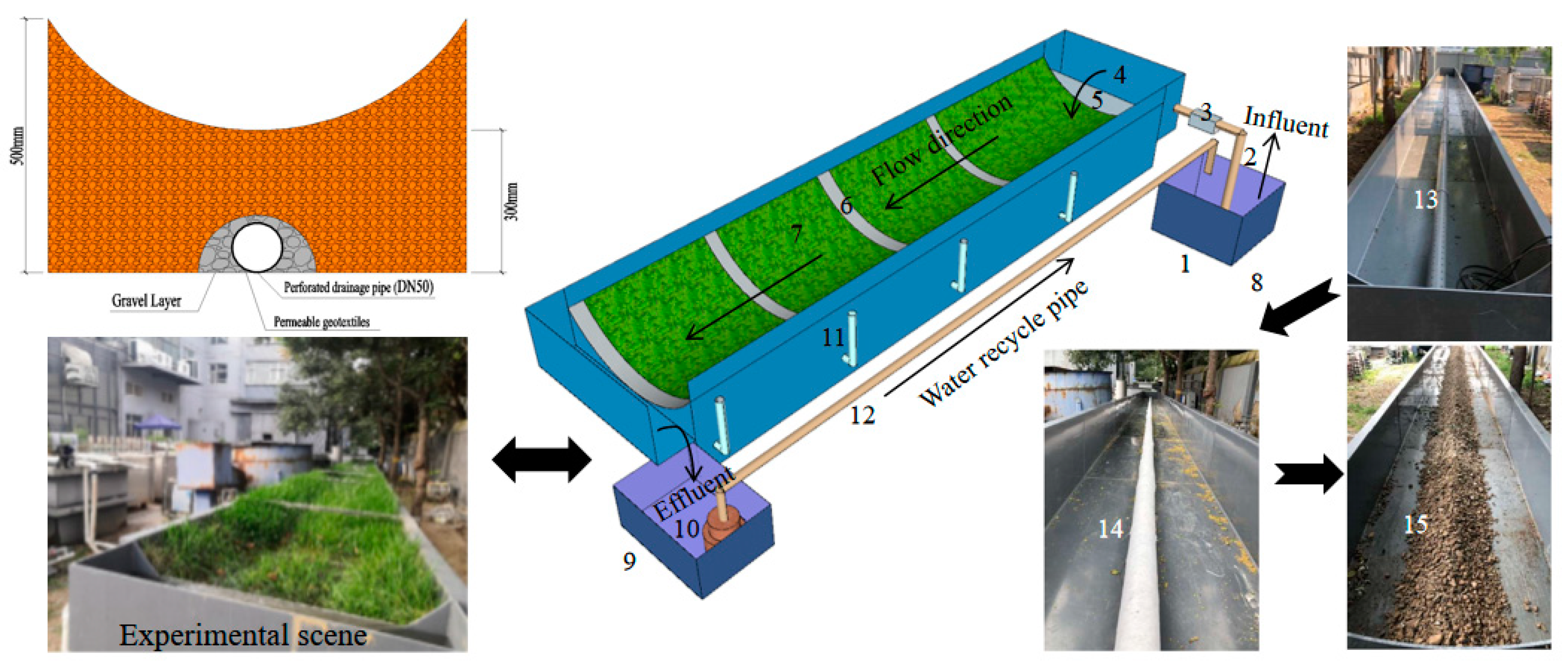
2.1. Experimental Device

The size of the experimental device was 20.0 m(L) × 1.0 m(B) × 0.5 m(H), as depicted in Figure 1. It featured a 2% longitudinal slope with a 1:3 ratio compared to its transverse slope. A perforated drainage pipe with a diameter of 50 mm, wrapped in permeable geotextile, was located at the center bottom of the grass swale. The perforated drainage pipe was surrounded by a gravel layer, which in turn was covered by planting soil with a minimum height of 300 mm in the center and a maximum of 500 mm at the edge. The cross-sectional design followed an arc shape. The device comprised inlet and outlet tanks, influent and water recycling pipes, and the grass swale. The grass swale was filled with sandy soil and planted with frugal grasses, achieving a 100% vegetation coverage. An electromagnetic flowmeter (RZYLDG, DN50) regulated the inflow rate in the inlet pipe. A pump (65WQK25-15-2.2) transferred runoff to the distribution cell, which then spilled runoff into the grass swale, with the effluent flowing into the harvesting cell. It was then channeled back to the inlet tank via the water recycle pump (65WQK20-10-1.5). The level gauge (RLS-7) automatically regulated these processes. The experiment’s duration depended on the time required for the grass swale’s flow and infiltration rates to stabilize, typically about 30 min, as shown in Figure 2. Yet, with an inflow rate of 1.00 m³/h, the duration extended to 60 min. Once the flow and infiltration rates in the grass swale stabilized, monitoring data were recorded. At this point, when the water content was saturated, Darcy’s law could be applied to calculate the infiltration rate.

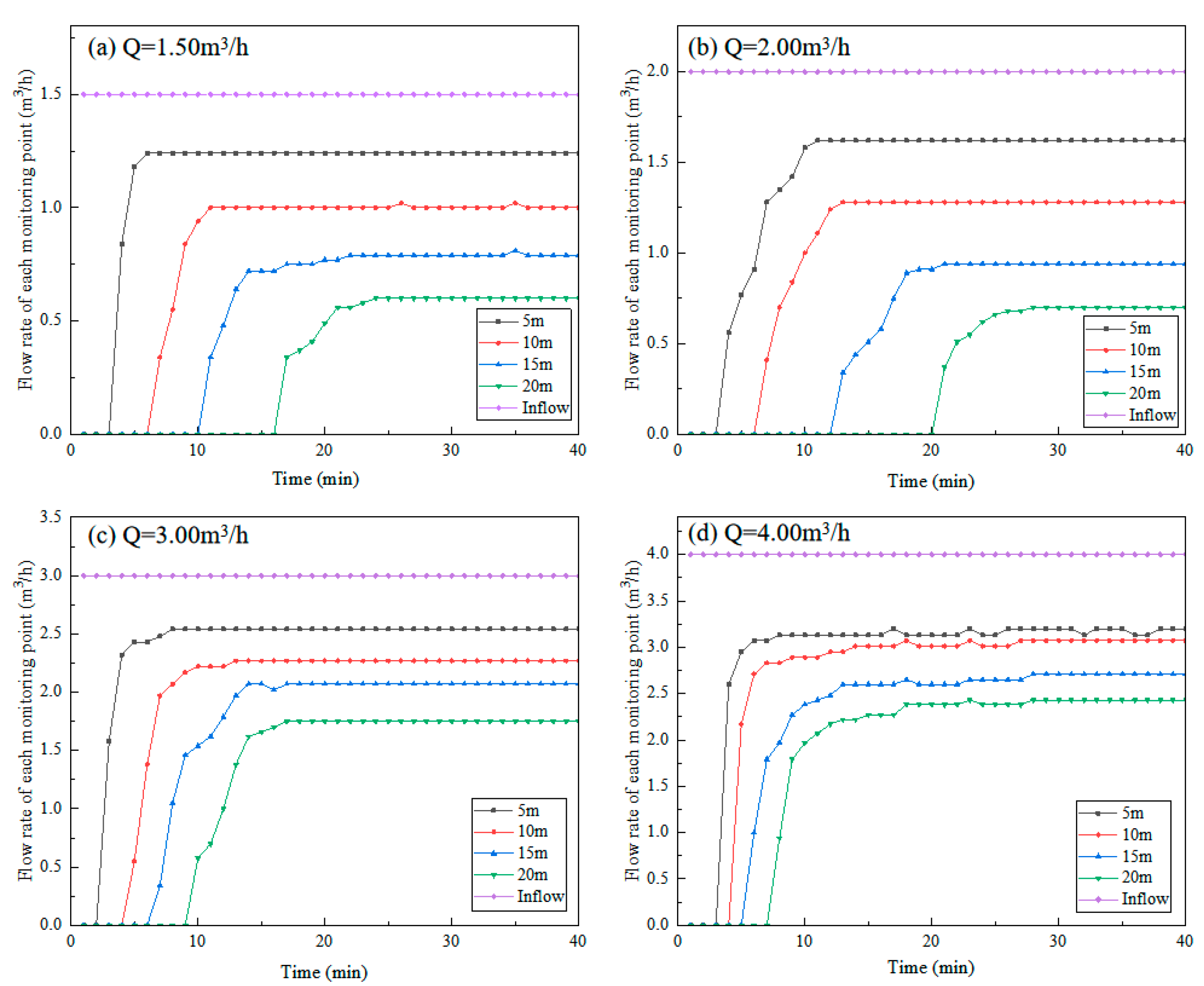
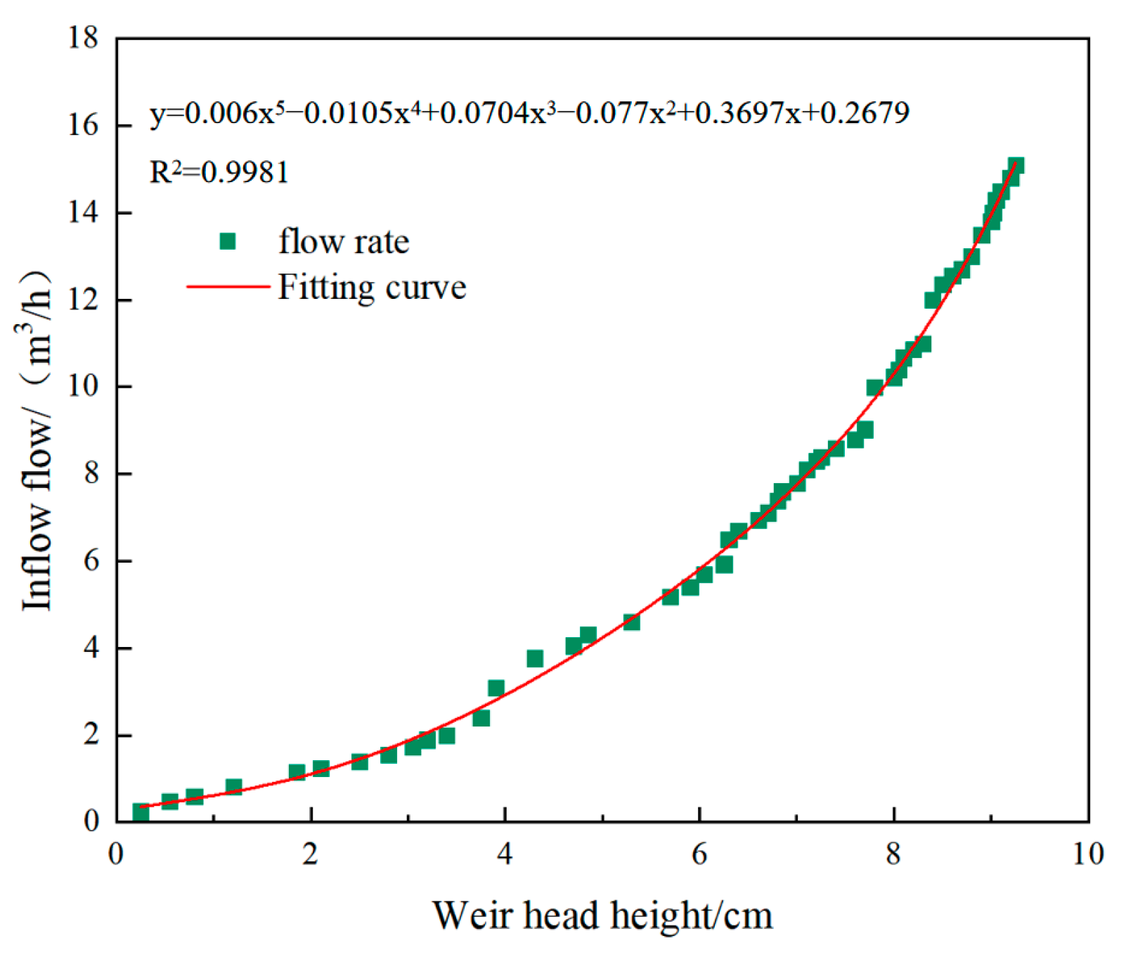
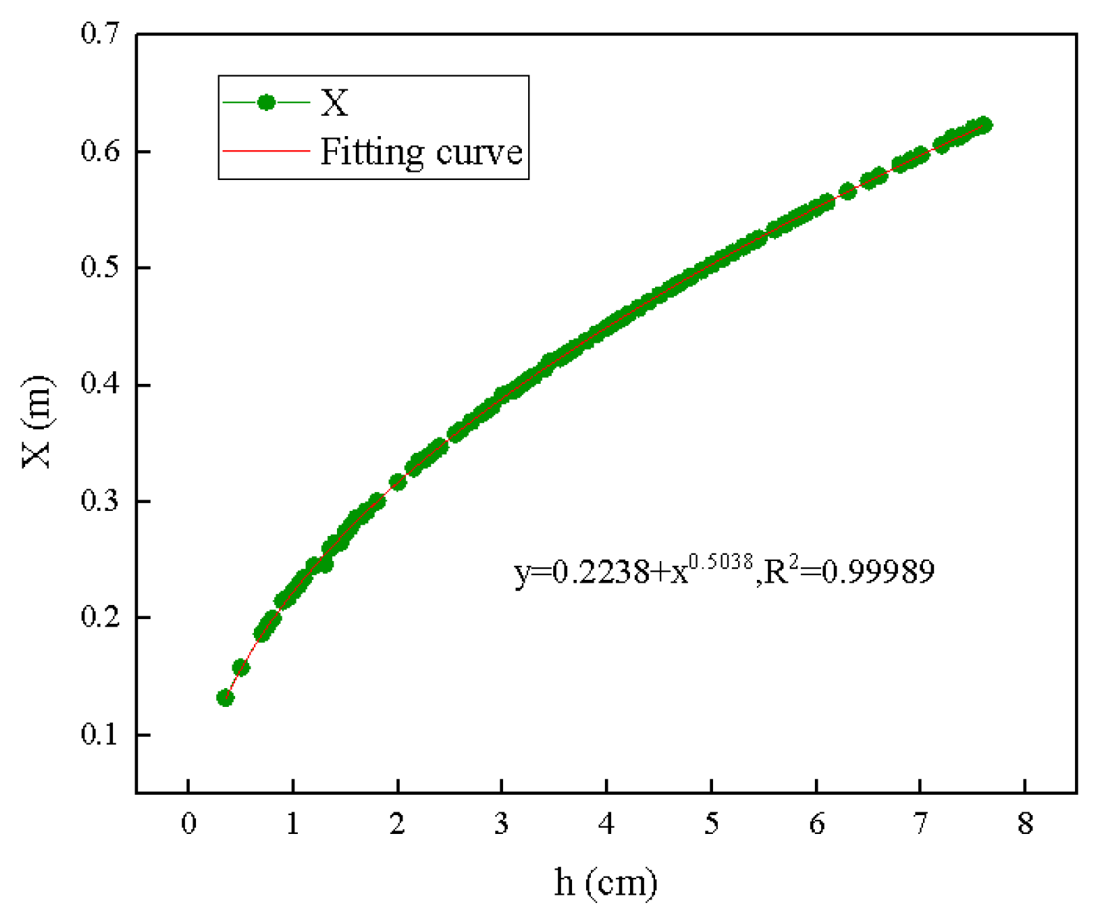
2.2. Flow Rate Measurement Method

A thin-walled weir was used for flow rate monitoring along the grass swales, as shown in Figure 3. The weir was triangular with an arc-shape. At the grass swale’s lowest point, directly in front of the weir, there was a connecting hole, 8 mm in diameter, linked to a monitoring tube. A steel ruler, affixed adjacent to the monitoring tube outside the grass swale, measured the water depth on the weir. The water depth on the weir was calculated as $h=h_3-∆h-0.02$. Notably, to minimize the triangular weir’s impact on overflow, a 2 cm gap was maintained from its lowest point to the grass swale’s bottom, with $∆h=h_2-h_1$. The change in water depth before and after the thin-walled weir was minimal, with a variation of less than 1 mm. Thus, the effect of the thin-walled weir on the flow dynamics along the grass swale was negligible.

Weir flow rates were calibrated in the laboratory: measurement of the inflow rate by means of an electromagnetic flow meter installed on the inlet pipe, and simultaneous measurement of the water depth over the thin-walled weir under different inflow rates, to obtain the corresponding relationship between water depth on the weir and the inflow rate. The correlation between the water depth h on the weir and the flow rate Q is illustrated in Figure 4. As the flow rate increases, there is a corresponding rise in the water depth. This relationship is described by the Q-h equation, denoted as Equation (1).

$$Q=0.0006h^5-0.011h^4+0.070h^3-0.077h^2+0.370h+0.268$$

(1)

where h is the water depth on the weir, h (cm).

Once the water depth on the weir was recorded, the flow rate in the grass swale at the corresponding position could be calculated using Equation (1). The data closely aligned with Equation (1), exhibiting an R² value of 0.998.

2.3. Manning’s Equation

The flow rate in grass swales is typically calculated using Manning’s equation [22,23,24], as represented by Equation (2).

$$Q=\frac{A{R}^{\frac{2}{3}}{i}^{\frac{1}{2}}}{n}$$

(2)

where Q (m³/s) is the flow rate, A (m²) is the cross-sectional area, R (m) is the hydraulic radius, i is the longitudinal slope of the grass swale, and n is the Manning’s coefficient, related to several factors including vegetation type and the degree of tortuousness in the grass swale.

Cowan [25] proposed a detailed method to calculate the Manning’s coefficient n, as represented by Equation (3).

$$n=(n_0+n_1+n_2+n_3+n_4)·m_5$$

(3)

where n is the Manning’s coefficient of grass swales, n₀ is related to permeable material types, n₁ reflects irregularity, n₂ reflects cross-sectional changes, n₃ is related to obstruction or pollutant interception settings, n₄ pertains to the influence degree of vegetation, and m₅ reflects the degree of twists and turns in the grass swale.

For the experimental grass swale with soil, n₀ was 0.020. Given the regular shape and unchanged cross-section, n₁ and n₂ were neglected. Since there were four weirs in the grass swale, n₃ was 0.06. With vegetation in the grass swale accounted for, n₄ was 0.08. Due to the absence of longitudinal curvature in the grass swale, m₅ was 1. Hence, n = (0.020 + 0 + 0 + 0.06 + 0.08) × 1 = 0.17.

The grass swale had a top width of 1 m and an arc-shaped cross-section with a radius of 0.625 m, as depicted in Figure 5. Utilizing the Pythagorean theorem for the water depth h, the hydraulic radius and water surface width can be determined using Equations (4) and (5).

$$r^2={(r-h)}^2+({\frac{b}{2})}^2$$

(4)

$$b=2·\sqrt{r^2-{(r-h)}^2}$$

(5)

where r is the radius of the arc corresponding to the cross-section of the grass swale, h is the water depth in the grass swale, and b is the water surface width of the grass swale.

Hence, we obtain Equation (6).

$$\mathit{cos}\left(\frac{\theta }{2}\right)=\frac{r-h}{r}$$

(6)

where θ is the arc angle corresponding to the water depth of the grass swale.

By substituting the relevant parameters of the grass swale into Equation (6), we determine the cosine value. This value is then referenced against a cosine angle comparison table to ascertain the θ value. Therefore, when the water depth is h, the wetted perimeter (X = θ·r) is calculated. Concurrently, the flow’s cross-sectional area A at water depth h is calculated using Equation (7).

$$A=\frac{\theta }{2\pi }·\pi r^2-\frac{b·\left(r-h\right)}{2}=\frac{\theta r^2}{2}-(r-h)·\sqrt{r^2-{(r-h)}^2}$$

(7)

Thus, by substituting the measured water depth from the weir into Equation (7), the flow’s cross-sectional area A can be determined. From there, the hydraulic radius r can be calculated, allowing for the calculation of the theoretical flow rate using Equation (2).

As depicted in Figure 6, the infiltration characteristics across the cross-section of the grass swale, which has a circular arc shape, indicate that at a water depth of h, the width of the water surface is L. This water depth diminishes progressively from the center towards the edges of the grass swale’s longitudinal slope.

The seepage volume Q_s can be calculated using the Darcy’s law (Equation (8)), provided the flow is linear, laminar, and stable. Generally, in mediums like sand and clay, the infiltration velocity is relatively low, and flow lines can be assumed to be nearly parallel, as depicted in Figure 6.

$$Q_s=KAJ$$

(8)

where K is the permeability coefficient, measured as 1.29 × 10⁻³ cm/s when J was 1 for v = K.

The infiltration area A along the grass swale can be approximated as a trapezoid for calculation purposes, ensuring equivalent area coverage as shown in Figure 7, which can be calculated using Equation (9).

$$A={\int }_0^L\frac{1}{2}(X+X^{\prime })dL$$

(9)

The infiltration process in the grass swale is characterized by one-dimensional vertical infiltration. Thus, the infiltration rate is calculated using Equation (10).

$$Q_s=KJ{\int }_0^L\frac{1}{2}(X+X^{\prime })dL$$

(10)

where Q_s is the infiltration rate within the grass swale, m³/s; K is the permeability coefficient, m/s; J is the hydraulic slope, the difference in water level along the grassed swale is less than 1 cm, and the difference of ∆h/l along the swale is negligible, so J can be considered to be approximately equal; X is the wet perimeter, m; X′ is the wet perimeter after the length change dL; and L is the grass swale’s length, m.

The presence of vegetation may have an impact on the flow’s cross-sectional area, thus affecting the wet perimeter. The relationship between the wet perimeter X and water depth h was derived from 88 groups of data obtained in the experiment, as presented in Figure 8. For an arc-shaped grass swale section with a width of 1 m, the relationship between the wet perimeter X and water depth h follows Equation (11), with a valid water depth range for Equation (11) being between 0.35 cm and 6.00 cm.

$$X=0.224h^{0.504}$$

(11)

3. Results and Discussion

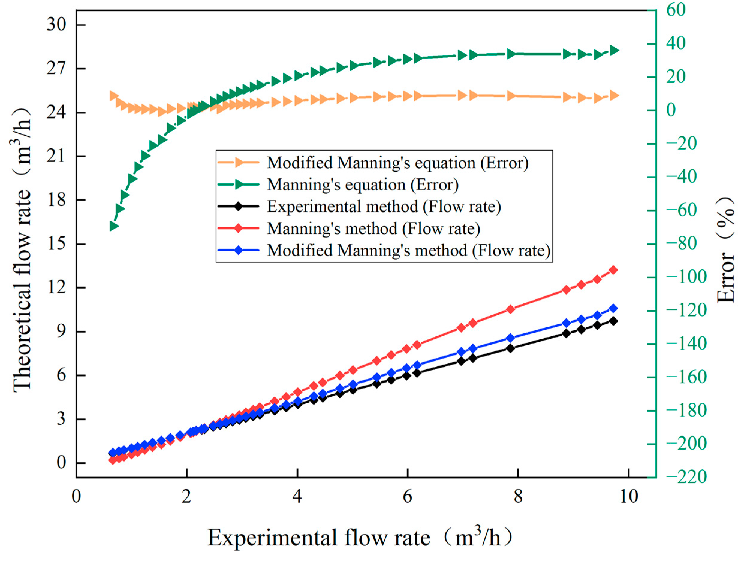
3.1. Comparison between Calculated Results and Experimental Data

The differences between theoretical calculation results from Manning’s equation and the experimental data are shown in Figure 9, illustrating that the discrepancy between measured values and theoretical predictions shifts from positive to negative as the inlet flow rate increases. At an inflow rate of 4.00 m³/h, the flow rate measured at various points along the grass swale was consistently lower than the theoretical flow rate, with a variance ranging from 0.01 to 0.61 m³/h. The smallest discrepancy between the measured and theoretical flow rates occurred at an inflow rate of 3.00 m³/h, with differences spanning from −0.24 to 0.19 m³/h. With inflow rates of 1.00 and 2.00 m³/h, the measured flow rates were always greater than the theoretical predictions. A likely reason is that as the runoff inflow rate increases, the wet perimeter within the grass swale expands, leading to a higher proportion of runoff infiltrating into the soil. Previous studies corroborate this, indicating that a significant majority of runoff, between 90% and 98% from rainfall, can penetrate into the soil through the grass swale [9]. In addition, dense turf is known to enhance soil permeability [26], and plant roots can locally boost hydraulic conductivity [27], especially at lower flow rates where retention and seepage significantly affect flow dynamics within the grass swale. Conversely, at higher flow rates, plant resistance, primarily due to leaf density, becomes a more dominant factor [14]. In this experiment, the abundance of foliage in the grass swale increased its resistance, preventing full infiltration and consequently raising water depths within the grass swale, which likely resulted in theoretical flow rates surpassing those measured.

The relationship between water depth h and the length of the grass swale L, as shown in

Table 1. The relationship of h-L and Q-L under different inflow rates.

		Fitting Formula
Q = 1.00 m3/h	h-L	h = −3.00 × 10−5L4 + 1.10 × 10−3L3 − 1.12 × 10−2L2 − 2.75 × 10−2L + 1.80
	Q-L	Q = −1.27 × 10−5L4 + 4.60 × 10−4L3 − 4.28 × 10−3L2 − 2.05 × 10−2L + 1.00
Q = 1.50 m3/h	h-L	h = 1.33 × 10−5L4 − 4.00 × 10−4L3 + 2.67 × 10−3L2 − 5.50 × 10−2L + 2.55
	Q-L	Q = 6.00 × 10−6L4 − 1.67 × 10−4L3 + 1.25 × 10−3L2 − 4.10 × 10−2L + 1.50
Q = 2.00 m3/h	h-L	h = 5.33 × 10−6L4 − 2.00 × 10−4L3 + 2.67 × 10−3L2 − 6.50 × 10−2L + 3.13
	Q-L	Q = 3.33 × 10−6 L4 − 1.27 × 10−4L3 + 2.12 × 10−3L2 − 5.78 × 10−2L + 2.00
Q = 3.00 m3/h	h-L	h = 2.67 × 10−6 L4 − 1.33 × 10−4L3 + 2.33 × 10−3L2 − 5.67 × 10−2L + 4.04
	Q-L	Q = 2.00 × 10−6L4 − 1.13 × 10−4L3 + 2.55 × 10−3L2 − 6.82 × 10−2L + 3.00
Q = 4.00 m3/h	h-L	h = 1.97 × 10−5L4 − 1.05 × 10−3L3 + 1.82 × 10−2L2 − 1.46 × 10−1L + 4.80
	Q-L	Q = 2.87 × 10−5L4 − 1.50 × 10−3L3 + 2.59 × 10−2L2 − 2.06 × 10−1L + 4.00

, uses a constant inflow Q = 4.00 m³/h as an example. This relationship is expressed by Equation (12).

$$h=(1.967\times {10}^{-5})L^4-0.001L^3+0.018L^2-0.146L+4.795$$

(12)

where h (m) is the water depth, and L (m) is the length of the grass swale.

By substituting Equation (12) into Equation (11), we obtain Equation (13). Further applying Equation (13) to Equation (10) allows us to derive the function X = f (L). With a flow rate of 4.00 m³/h, the infiltration rate is determined by Equation (14).

$$X=f\left(L\right)=0.224[{(1.967\times {10}^{-5})L^4-0.001L^3+0.018L^2-0.146L+4.795]}^{0.504}$$

(13)

$$\begin{array}{l}Q=KJ{\int }_0^L\frac{1}{2}\left[0.48+f\left(L\right)\right]dL\\ =KJ{\int }_0^L\{0.112\left[{\left(1.967{\times 10}^{-5}\right)L^4-0.001L^3+0.018L^2-0.146L+4.795]}^{0.504}+0.24\right\}dL\\ =0.112KJ{\int }_0^L[{\left(1.967{\times 10}^{-5}\right)L^4-0.001L^3+0.018L^2-0.146L+4.795]}^{0.504}dL+0.24KJL\end{array}$$

(14)

Since there is no explicit function for Equation (14) that conforms to the experimental conditions, a numerical solution method was adopted to approximate the solution, as shown in Figure 10.

Equation (13) can be further simplified into Equation (15)

$$Q=0.112KJ[5.71\times {10}^{-2}·L+6.484\times {10}^{-3}·{\left(L-30\right)}^2+1.442\times {10}^{-4}·{\left(L-30\right)}^3-8.891\times {10}^{-6}·{\left(L-30\right)}^4]+0.24KJL$$

(15)

where Q is the infiltration rate in the grass swale, m³/s; K is the permeability coefficient, measured as 1.29 × 10⁻⁵ m/s; J is the hydraulic slope; X is the wet perimeter, m; A is the infiltration cross section area, m²; and L is the length of the grass swale, m.

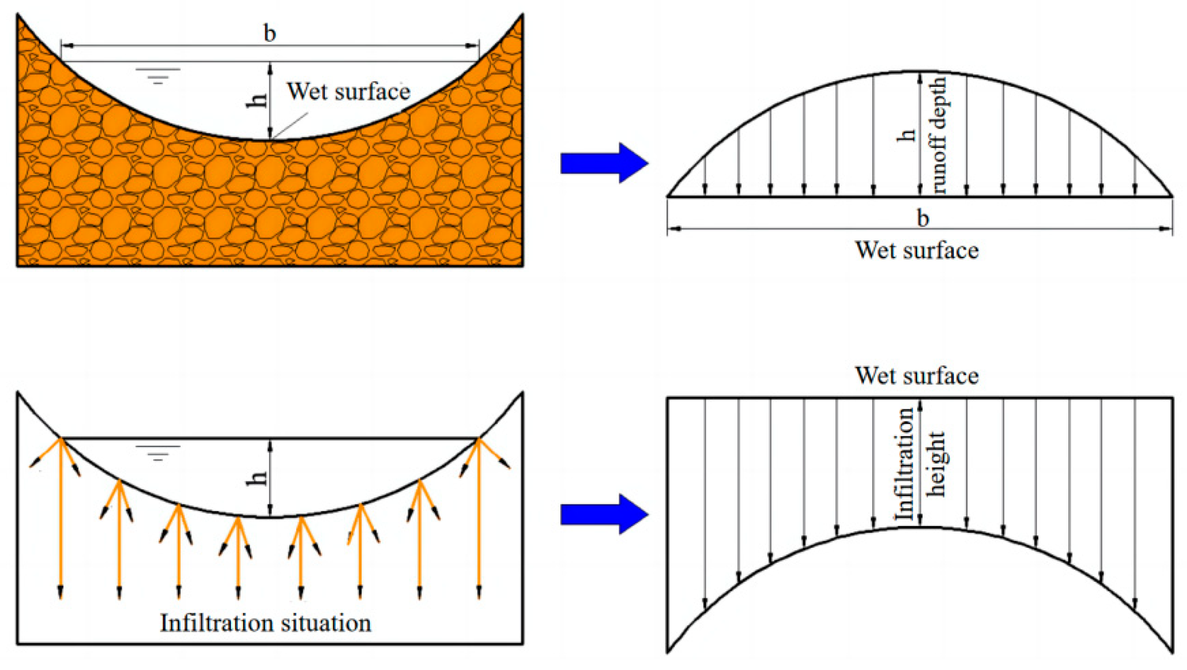
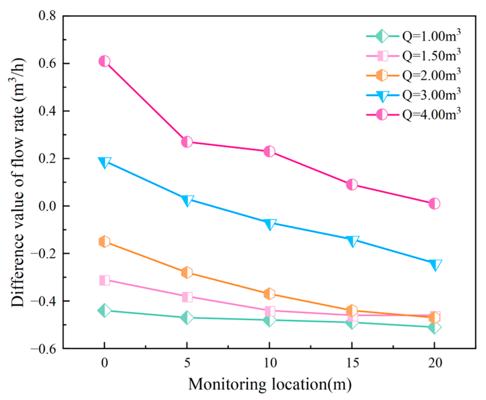
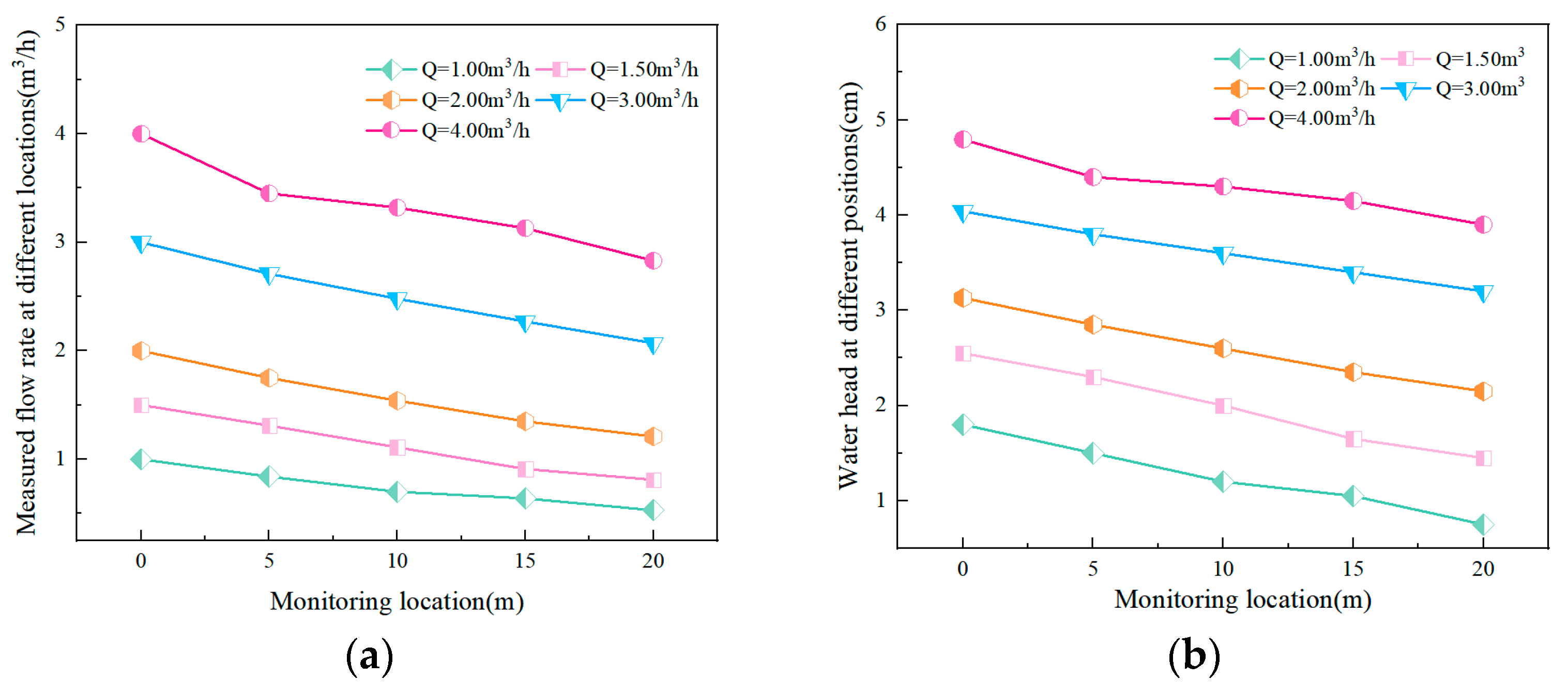
3.2. Characteristics of Flow Rate and Water Depth along the Grass Swale

The changing characteristics of the flow rate along the grass swale are shown in Figure 11a. It can be seen that the effluent flow rate gradually increases from 0.53 to 2.83 m³/h as the inflow rate increases from 1.00 to 4.00 m³/h. Furthermore, the flow rate reduction per unit distance gradually increases from 0.024 to 0.059 m³/h, possibly because the infiltration area and seepage volume also increase as the flow rates rise. A slight fluctuation in the flow rate reduction along the grass swale was found when the inflow rate was at 1.00 and 4.00 m³/h. This may be due to differences in seepage loss and resistance along the grass swale under varying flow rates. The experimental results align with the findings of Shen et al. [28]. The change in water depth along the grass swale is shown in Figure 11b. The water depth at the outlet increases from 0.75 to 3.90 cm when the inflow rate increases from 1.00 to 4.00 m³/h. However, the reduction in water depth per unit distance does not show obvious regularity. The reason may be that the increase in ∆h requires different ∆Q at varying initial water depths, given that the cross-section of the grass swale was arc-shaped.

Inflow rates significantly affect the flow reduction rate along the grass swale. The experiment results of the flow reduction rate in the grass swale at various inflow rates are shown in

Table 2. Flow reduction rate along the grass swale under different inflow rates (%).

Distance from Inlet (m)	Inflow Rate (m3/h)
	1.00	1.50	2.00	3.00	4.00
5	16.00	12.67	12.50	9.67	8.75
10	30.00	26.00	23.00	17.33	17.00
15	36.00	39.33	32.50	24.33	21.75
20	47.00	46.00	39.50	31.00	29.25

. It can be seen that as the inflow rate increases, the flow reduction rate decreases. Specifically, at a distance of 5 m from the inlet, the runoff reduction rate decreases from 16.00% to 8.75% as the inflow rate increases from 1.00 to 4.00 m³/h. Similarly, at the outlet, the reduction rate drops from 47.00% to 29.25%. This trend likely occurs because the increase in the infiltration rate becomes negligible as inflow rates rise, resulting in a lower flow reduction rate. Additionally, the flow reduction rate increases along the length of the grass swale. For instance, it increases from 16.00% to 47.00% as the length increases from 5 to 20 m when the inflow is 1.00 m³/h, attributed to flow loss over distance. Similar to this study, Stagge [29] found that the overall stormwater flow reduction rate by the grass swale is about 46 to 54%, and Shafique et al. [30] found the flow reduction rate range of 40 to 75%.

3.3. Modified Method for Flow Rate Calculation along the Grass Swale

A linear relationship between the measured and theoretical flow rates in the grass swale was established by fitting data from the experiments with varying inflow rates. The relationship is given by Equation (16).

$$Q_{exp}=a\prime Q_{theory}+b\prime$$

(16)

where $Q_{exp}$ is the measured flow rate, and $Q_{theory}$ is the theoretical flow rate.

The fitting values of a′ and b′ across various flow conditions are listed in

Table 3. Fitting parameters of Equation (16).

Inflow Rate (m3/h)	a′	b′	R2
1.00	0.978	0.462	0.996
1.50	0.824	0.526	0.999
2.00	0.773	0.579	0.999
3.00	0.740	0.638	0.999
4.00	0.709	0.725	0.999

, indicating a strong fit with an R² that exceeds 0.99 for all inflow rates. For an inflow rate of 1.00 m³/h, a′ decreases as the inflow rate increases, while b′ increases with the inflow rate. Specifically, a′ decreases from 0.978 to 0.709 as Q increases from 1.00 to 4.00 m³/h, while b′ rises from 0.462 to 0.725. Consequently, the slope of the correlation curve between the measured and theoretical flow rates diminishes as the inflow rate increases, and the intercept correspondingly rises.

To establish the relationship between the measured and theoretical flow rates within the grass swale, the theoretical flow rate under different inflow rates was plotted on the x-axis against the measured flow rate on the y-axis for correlation analysis, as shown in Figure 12. The data aligned well with the linear relationship, evidenced by a coefficient of determination R² = 0.9986, as represented by Equation (17).

$$Q_{exp}=0.759Q_{theory}+0.565$$

(17)

By combining Manning’s equation from Equation (7) with Equation (17), we obtained the modified Manning’s equation, as shown in Equation (18).

$$Q_{exp}=0.759\frac{{[\frac{\theta r^2}{2}-(r-h)·\sqrt{r^2-{\left(r-h\right)}^2}]}^{5/3}{i}^{1/2}}{n·{\theta r}^{2/3}}+0.565$$

(18)

Typically, the longitudinal slope i and roughness coefficient n of the grass swale remains constant. For an arc-shaped cross-section, the corresponding radius r correlates with the width d and the shape of the cross-section. The arc angle θ is determined by Equation (6) given the water depth h. Substituting i, n, θ, r into Equation (18) allows for the calculation of the flow rate along the grass swale for a specific water depth.

The modified Manning’s equation was validated against the experimental results for inflow rates ranging from 0.66 to 9.72 m³/h. The validation process involved calculating the modified theoretical flow rate using the experimentally measured water depth and roughness coefficient via Equation (18), followed by comparison to the measured flow rate. The discrepancy between the two values is quantified by the error percentage, as expressed in Equation (19).

$$Error=\frac{Q_{theory}-Q_{exp}}{Q_{exp}}·100\%$$

(19)

The error analysis comparing measured flow rates with those predicted by both the traditional and modified Manning’s equations across various inflow rates is illustrated in Figure 13. It is observed that the modified Manning’s equation is more precise for estimating flow rates in the grass swale, especially for inflow rates less than 4.00 m³/h, making it a superior method for calculating flow rates in the grass swale. Specifically, the error between experimental measured and modified Manning’s equation calculated results ranges from −0.71 to 9.05%, varying from −0.71 to 5.43% when the inflow rate ranges from 1.00 to 4.00m³/h. However, the error increases for inflow rates exceeding 4.00 m³/h, rising from 5.86 to 9.05% as the inflow rate increases from 4.00 to 9.72 m³/h. However, the error between experimental measured flow rates and those calculated by Manning’s equation escalates with higher inflow rates, spanning from −69.30 to 36.00% as the inflow rate increases from 0.5 to 8 m³/h. This indicates a significant discrepancy when using the traditional Manning’s equation for calculating flow rates in the grass swale. Meanwhile, the error for results calculated by Manning’s equation remains small, between −1.94 and 11.24%, for inflow rates from 2.00 m³/h to 3.00 m³/h. Thus, the modified Manning’s equation proves effective for calculating flow rates in the grass swale.

4. Summary and Conclusions

The hydraulic characteristics of grass swales under low inflow rate conditions were systematically investigated in this study. Flow rate losses and changes in grass resistance along the grass swale were inconsistent with the assumptions of Manning’s equation. Therefore, using Manning’s equation to calculate flow rates in grass swales incurred significant errors, with biases shifting from negative to positive as inflow rates increased. The smallest discrepancy between measured flow rates and those calculated using Manning’s equation occurred at an inflow rate of approximately 3.00 m³/h, with deviations expanding as flow rates varied. Water depth and flow rates in the grass swale gradually decrease with increasing distance. Infiltration losses along the grass swale varied greatly under different inflow rates. An equation for calculating the infiltration rates was derived using Darcy’s law and experimental data. A modified method based on Manning’s equation for calculating flow rates in grass swales was proposed. Results from the modified Manning’s equation closely matched experimental data with errors ranging from −0.71 to 9.05%, compared to −69.30 to 36.00% for the original Manning’s equation. Consequently, the modified Manning’s equation is more precise for estimating flow rates in grass swales, particularly for inflow rates below 4.00 m³/h, making it a superior method. This work offers a more accurate method for calculating drainage capacity, TSS migration, and erosion prevention in grass swales.

This study focused solely on the impact of infiltration loss on flow rates along grass swales. However, the interactive process of infiltration loss and resistance change along grass swales requires further quantification. Vegetation density, which significantly impacts resistance changes, should be further investigated as a variable. Different media or soil compaction levels result in varying K values, necessitating adjustment to these values. Rainfall parameters, including rainfall intensity, duration, and interval, are crucial factors affecting flow rates along grass swales. While a constant flow rate was adopted in this study, the nonuniform inflow rate hydrograph in actual rainfall events suggests further investigation of grass swales’ hydraulic characteristics under varying conditions is necessary.

References

1. Margerum, R.D. Integrated Approaches to Environmental Planning and Management. J. Plan. Lit. 1997, 11, 459–475. [Google Scholar] [CrossRef]
2. Zhao, H.; Zou, C.; Zhao, J.; Li, X. Role of Low-Impact Development in Generation and Control of Urban Diffuse Pollution in a Pilot Sponge City: A Paired-Catchment Study. Water 2018, 10, 852. [Google Scholar] [CrossRef]
3. Che, W.; Zhao, Y.; Yang, Z.; Li, J.; Shi, M. Integral stormwater management master plan and design in an ecological community. J. Environ. Sci. 2014, 26, 1818–1823. [Google Scholar] [CrossRef]
4. Wang, J.; Wang, M.; Che, W.; Li, J.; Zhao, Y.; Wang, W. Discussion on key issues of low-impact development rainwater system construction. China Water Wastewater 2015, 31, 6–12. [Google Scholar] [CrossRef]
5. Pitt, R.; Nara, Y.; Kirby, J.; Durrans, S. Particulate Transport in Grass Swales; Low Impact Development, 2012; pp. 191–204. Available online: https://ascelibrary.org/doi/10.1061/41007%28331%2917 (accessed on 18 March 2024). [CrossRef]
6. Davis Allen, P. Field Performance of Bioretention: Hydrology Impacts. J. Hydrol. Eng. 2008, 13, 90–95. [Google Scholar] [CrossRef]
7. Kirby Jason, T.; Durrans, S.R.; Pitt, R.; Johnson Pauline, D. Hydraulic Resistance in Grass Swales Designed for Small Flow Conveyance. J. Hydraul. Eng. 2005, 131, 65–68. [Google Scholar] [CrossRef]
8. Cheng, N.-S.; Nguyen Hoai, T. Hydraulic Radius for Evaluating Resistance Induced by Simulated Emergent Vegetation in Open-Channel Flows. J. Hydraul. Eng. 2011, 137, 995–1004. [Google Scholar] [CrossRef]
9. Ahmed, F.; Gulliver John, S.; Nieber John, L. Determining Infiltration Loss of a Grassed Swale. In Proceedings of the World Environmental and Water Resources Congress 2014, Portland, Oregon, 1–5 June 2014; pp. 8–14. [Google Scholar] [CrossRef]
10. Yang, F.; Fu, D.; Zevenbergen, C.; Boogaard, F.C.; Singh, R.P. Time-varying characteristics of saturated hydraulic conductivity in grassed swales based on the ensemble Kalman filter algorithm—A case study of two long-running swales in Netherlands. J. Environ. Manag. 2024, 351, 119760. [Google Scholar] [CrossRef] [PubMed]
11. Deletic, A. Modelling of water and sediment transport over grassed areas. J. Hydrol. 2001, 248, 168–182. [Google Scholar] [CrossRef]
12. Deletic, A.; Fletcher, T.D. Performance of grass filters used for stormwater treatment—A field and modelling study. J. Hydrol. 2006, 317, 261–275. [Google Scholar] [CrossRef]
13. Zhang, W.; Hao, W.; Yan, W.; LI, S. Influence of Influent Load on Stormwater Runoff Control in Grassed Swales. Water Resour. Power 2020, 38, 22–25. [Google Scholar]
14. Järvelä, J. Determination of flow resistance caused by non-submerged woody vegetation. Int. J. River Basin Manag. 2004, 2, 61–70. [Google Scholar] [CrossRef]
15. Hu, Y.; Huai, W.; Han, J. Analytical solution for vertical profile of streamwise velocity in open-channel flow with submerged vegetation. Environ. Fluid Mech. 2013, 13, 389–402. [Google Scholar] [CrossRef]
16. Bi, Y.; Zou, H.; Zhu, C. Dynamic monitoring of soil bulk density and infiltration rate during coal mining in sandy land with different vegetation. Int. J. Coal Sci. Technol. 2014, 1, 198–206. [Google Scholar] [CrossRef]
17. Rujner, H.; Leonhardt, G.; Marsalek, J.; Perttu, A.-M.; Viklander, M. The effects of initial soil moisture conditions on swale flow hydrographs. Hydrol. Process. 2018, 32, 644–654. [Google Scholar] [CrossRef]
18. Chen, L.; Liu, Q.; Li, J. Study on the Runoff Generation Process on the Slope with Numerical Method. J. Sediment Res. 2001, 4, 61–67. [Google Scholar] [CrossRef]
19. Iverson, R.M. Landslide triggering by rain infiltration. Water Resour. Res. 2000, 36, 1897–1910. [Google Scholar] [CrossRef]
20. Rujner, H.; Leonhardt, G.; Marsalek, J.; Viklander, M. High-resolution modelling of the grass swale response to runoff inflows with Mike SHE. J. Hydrol. 2018, 562, 411–422. [Google Scholar] [CrossRef]
21. García-Serrana, M.; Gulliver John, S.; Nieber John, L. Calculator to Estimate Annual Infiltration Performance of Roadside Swales. J. Hydrol. Eng. 2018, 23, 04018017. [Google Scholar] [CrossRef]
22. Wilson, C.A.M.E. Flow resistance models for flexible submerged vegetation. J. Hydrol. 2007, 342, 213–222. [Google Scholar] [CrossRef]
23. Seo, Y.; Park, S.Y.; Schmidt, A.R. Implication of the flow resistance formulae on the prediction of flood wave propagation. Hydrol. Sci. J. 2016, 61, 683–695. [Google Scholar] [CrossRef]
24. Elmoaty, M.; Elsamman, T. Manning roughness coefficient in vegetated open channels. Water Sci. 2020, 34, 121–128. [Google Scholar] [CrossRef]
25. Cowan, W.L. Estimating Hydraulic Roughness Coefficients. Agric. Eng. 1956, 121, 473–475. [Google Scholar]
26. Yousef, Y.A.; Wanielista, M.P.; Harper, H.H.; Pearce, D.; Tolbert, R.D. Best Management Practices: Removal of Highway Contaminants by Roadside Swales; Final Report; University of Central Florida, Florida Department of Transportation: Orlando, FL, USA, 1985; p. 166. [Google Scholar]
27. Deletic, A. Sediment Behaviour in Overland Flow over Grassed Areas; University of Aberdeen (United Kingdom): Aberdeen, UK, 2000. [Google Scholar]
28. Davis, A.P.; Stagge, J.H.; Jamil, E.; Kim, H. Hydraulic performance of grass swales for managing highway runoff. Water Res. 2012, 46, 6775–6786. [Google Scholar] [CrossRef]
29. Stagge, J. Field Evaluation of Hydrologic and Water Quality Benefits of Grass Swales for Managing Highway Runoff. Master’s Thesis, Department Civil & Environmental Engineering, University of Maryland, College Park, MD, USA, 2006. [Google Scholar]
30. Shafique, M.; Kim, R.; Kyung-Ho, K. Evaluating the Capability of Grass Swale for the Rainfall Runoff Reduction from an Urban Parking Lot, Seoul, Republic of Korea. Int. J. Environ. Res. Public Health 2018, 15, 537. [Google Scholar] [CrossRef]
Figure 1. Schematic diagram and photos of the experimental device (1—inlet tank; 2—inflow pipe; 3—electromagnetic flow meter; 4—distribution cell; 5—overflow baffle; 6—weir; 7—grass swale; 8—inlet tank; 9—outlet tank; 10—pump; 11—monitoring tube; 12—water recycling pipe; 13—PVC perforated drainage pipe; 14—permeable geotextiles; 15—gravel layer).
Water 16 01613 g001
Figure 2. Flow rate changing along grass swales with time elapse under different inflow rates.
Water 16 01613 g002
Figure 3. Water depth monitoring method of the triangular weir.
Water 16 01613 g003
Figure 4. The relationship between flow rate and water depth on weir.
Water 16 01613 g004
Figure 5. Sectional dimensions of the grass swale.
Water 16 01613 g005
Figure 6. The water depth at each position of the grass swale’s cross section.
Water 16 01613 g006
Figure 7. Infiltration area with constant inflow.
Water 16 01613 g007
Figure 8. Wet perimeter and water depth fitting curve.
Water 16 01613 g008
Figure 9. Difference between theoretical and measured flow rate along the grass swale.
Water 16 01613 g009
Figure 10. Fitting curve of the integral result of the infiltration rate.
Water 16 01613 g010
Figure 11. Changes of flow rate (a) and water depth (b) along the grass swale.
Water 16 01613 g011
Figure 12. Fitting results of measured and theoretical flow rate in the grass swale.
Water 16 01613 g012
Figure 13. Error analysis of flow rates with different methods.
Water 16 01613 g013