Abstract
This paper presents an original approach to predicting oil slick movement and dispersion at the water surface. Special emphasis is placed on the impact of evolving hydro-meteorological conditions and the thickness of the oil spill layer. The main gap addressed by this study lies in the need for a comprehensive understanding of how changing environmental conditions and oil thickness interact to influence the movement and dispersion of oil slicks. By focusing on this aspect, this study aims to provide valuable insights into the complex dynamics of oil spill behaviour, enhancing the ability to predict and mitigate the environmental impacts of such incidents. Self-designed software was applied to develop and modify previously established mathematical probabilistic models for predicting changes in the shape of the oil trajectory. First, a semi-Markov model of the process is constructed, and the oil thickness is analysed at the sea surface over time. Next, a stochastic-based procedure to forecast the horizontal movement and dispersion of an oil slick in diverse hydro-meteorological conditions considering a varying oil layer thickness is presented. This involves determining the trajectory and movement of a slick domain, which consists of an elliptical combination of domains undergoing temporal changes. By applying the procedure and program, a short-term forecast of the horizontal movement and dispersion of an oil slick provided its trajectory at the Bornholm Basin of the Baltic Sea within two days. The research results obtained are preliminary prediction results, although the approach considered in this paper can help responders understand the scope of the problem and mitigate the effects of environmental damage if the oil discharge reaches sensitive ecosystems. Finally, further perspectives of this research are given.
1. Introduction
A crucial matter concerning port and shipping operations is the prevention of oil leaks that pose threats to the environment and the minimisation of the consequences of their spread after accidents or incidents [1,2]. In recent years, significant advances in computing power and data analysis techniques have been made. This has allowed for the development of more accurate and efficient models which have proven invaluable for mitigating the environmental impact of oil spills [3,4]. There are various methods described in the literature for detecting the area of an oil slick and predicting its trajectory [5]. Many approaches are presented in [6,7,8], like D-WAQ PART, GNOME, MEDSLINK-II, MIKE Module, MOTHY, OpenDrift/OpenOil, OSCAR, POSEIDON, SIMAP, SPILLCALC, and VOILS. Some methods can also use real data reads e.g., from a ship’s sensors [4]. In the case of oil thickness and fate modelling [7], GNOME provides a focus on surface transport, with for the ability to model 3D particle transport influenced by winds, currents, and tides. Its integration with the ADIOS oil database offers algorithms for oil weathering, but it primarily emphasises surface and near-surface processes. On the other hand, OSCAR stands out for its detailed modelling of oil fate and effects, considering multiple pseudo-components of oil and their transport and weathering across all environmental segments. This model comprehensively addresses the vertical and horizontal dispersion of oil and degradation and sedimentation processes, making it highly suitable for detailed oil thickness and fate analyses throughout the water column and on the seafloor. SIMAP is geared towards strategic planning and post-spill assessments, with a strong focus on the entire water column. It provides simulations of oil spill trajectory, fate, transport, and biological impacts, incorporating complex interactions such as oil dissolution, sedimentation, and effects on wildlife. This model is ideal for environmental impact assessments and offers detailed insights into oil thickness and distribution in the water column. All the three mentioned models additionally use mathematical methods based on a probabilistic approach to represent uncertain outcomes [9]. SIMAP and OSCAR can be used in probabilistic or deterministic mode, while GNOME includes stochastic components and uncertainty algorithms regarding the perturbation of current and wind fields [7,10].
OSCAR’s detailed approach to simulating the chemical fate of oil across all environmental compartments can result in high computational demands, potentially limiting its accessibility or utility in rapid response scenarios without adequate computational resources [7]. While OSCAR’s comprehensive nature is a strong point, it might also limit its flexibility. The model’s detailed mechanisms, which are a boon for thorough analysis, could hinder its quick adaptation or application to vastly different spill scenarios without significant calibration. While OSCAR’s and SIMAP’s capability to run in both stochastic and deterministic modes is an advantage, finding the right balance between these modes for specific scenarios can be challenging. Overreliance on one mode may not accurately reflect the complexity of real-world oil spill dynamics. Although GNOME includes uncertainty algorithms, the extent and sophistication of these stochastic elements compared to real-world complexities might not capture all the variabilities in environmental conditions.
In this paper, a model of oil slick horizontal movement and dispersion in diverse hydro-meteorological conditions is presented and self-written software is proposed, expanding my previous works [11,12,13] by considering variations in oil layer thickness over time. The primary focus of this study is to bridge a gap in our understanding by comprehensively exploring how changing environmental conditions and oil thickness interact to influence the movement and dispersion of oil slicks. Focus is placed on exploring variations in oil layer thickness rather than solely concentrating on other factors, such as the physical characteristics of the oil. Additionally, the method is innovative due to its specific focus on modelling the thickness of the oil explicitly. It clearly broadens the range of available stochastic approaches used in this field. Moreover, stochastic semi-Markov models can be used to model a wider range of objects for which the time spent in a state is not necessarily exponential, as in the Markov approach [14]. In this paper, a novel approach is introduced, and the changeable oil slick thickness τ, i.e., τ = τk(t), at each hydro-meteorological state k and for t ∈ ⟨0,T⟩ is assumed and added to the model. Such an approach seems reasonable as the oil slick becomes thinner over time on the open sea. This model allows for a more nuanced understanding of the spill’s impact, enabling proactive measures to ensure rapid response and containment efforts. Using real-time hydro-meteorological data allows for the immediate forecasting of likely outcomes and the modification of response strategies to reduce the impact of oil spills, while acknowledging the complex interplay between water systems and human activities emphasizes the importance of water dynamics in controlling spill spread and mitigation efforts [15,16].
The remainder of this paper is organised as follows. Section 2 presents two main factors affecting oil slick movement and spread. In Section 2.1, the effect of oil slick thickness on predicting its trajectory is considered, and in Section 2.2, hydrological and meteorological conditions are analysed. Section 3 explains the research methodology and describes the probabilistic model used in the oil slick horizontal movement and dispersion investigation. First, a stochastic model of hydro-meteorological conditions is constructed. Next, a two-dimensional stochastic process used to describe the oil slick’s central point position is defined. The parametric equations of its drift trend curve are presented for different hydro-meteorological conditions and considering a change in the thickness of the oil slick layer over time. A model and a procedure are created for stochastic oil slick horizontal movement and dispersion. Section 4 presents the application and the results. Section 4.1 and Section 4.2 justify the selection of the Bornholm Basin in the Baltic Sea and analyses waves and winds in this area. Section 4.3 and Section 4.4 present input data for the model. In Section 4.5, the procedure is applied to evaluate the trajectory of a hypothetical oil slick leaked into the Bornholm Basin of the Baltic Sea based on provided hydro-meteorological data. In Section 5, a discussion of the results derived from the presented approach and suggestions for possible future research directions are provided. Section 6 summarises the results.
2. Factors Affecting Oil Slick Movement and Spreading
2.1. Oil Slick Thickness at the Sea Surface
There are about thirty approaches overall to remotely determining the thickness of an oil spill [17]. Most had never proceeded after the first paper acceptance. Several good ideas have been developed, but more research and validation are needed. Although sometimes validation has been carried out, the models’ performance in novel or less-studied environmental contexts or spill scenarios could be a limitation. Moreover, there are only two effective methods for digitally assessing oil thickness: laser–acoustic measurements and passive microwave radiometry [18]. At this moment, microwave radiometry has been developed and commercialised. However, microwave techniques may not work if the oil contains water.
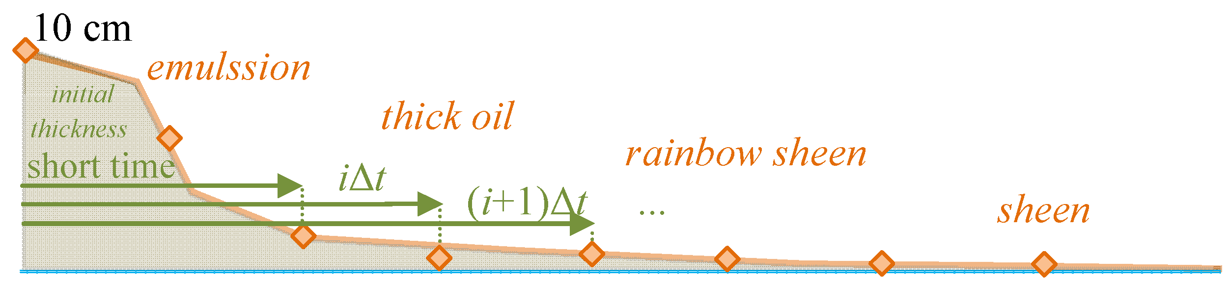
When oil spills, it begins as a single slick and quickly spreads across the surface of the sea [19]. Spreading is rarely consistent, and wide ranges in oil thickness are usual. A given area’s oil layer thickness can be roughly determined visually because the colour of the oil on the sea surface is typically directly related to its thickness (Figure 1). In terms of oil physical characteristics, emulsions, thick oil, rainbow sheens, and sheens exist under favourable observation conditions. The most prevalent type of oil that is commonly visible in the later stages of a spill is a sheen, which is a very thin layer of oil (less than 3 · 10−3 mm thick) floating on the water’s surface. Visually, estimations have been limited to thicknesses insights into sheens and rainbow sheens (thin sheens can be identified fairly reliably). Regretfully, the majority of oil is in a thicker area consisting of a slick, but this is manageable and recoverable. Sheens with rainbow colours are the only slicks which clearly indicate thickness. However, some heavy petroleum products and crude oils are exceptionally viscous and tend not to spread much, instead remaining in rounded patches. Crude oils can spread to a thickness of approximately 0.3 mm within twelve hours [19]. Oil spreads and disintegrates more quickly in harsher environments. A slick can start to break up after a few hours and will then form narrow bands or windrows parallel to the wind direction due to wind, wave movement, and water turbulence. A one-ton oil spill can spread over a 50 m radius in about ten minutes, creating a slick that is ten millimetres thick. As the oil spreads, it becomes thinner (less than one millimetre), eventually even covering 10 square kilometres [19].

Figure 1.
Average oil thickness at the sea surface over time in mild hydro-meteorological conditions [17].
Most oil slick profiles presented in Figure 1 have a the shape of a circle or an ellipse from a top view. The average oil thickness at the sea surface over time in mild hydro-meteorological conditions depicted in Figure 2 can range from 10 cm to almost 0; however, the initial thickness of 10 cm can only last for a few minutes and quickly drops to 1–2 mm [17].

Figure 2.
Existing theoretical oil slick profiles based on the concept of block, egg, flat, and wedge profiles [18].
To evaluate the impact of winds and waves on the horizontal movement and dispersion of an oil slick in a considered area, states of the process of changing hydro-meteorological conditions for the considered area are described in the next section.
2.2. Oil Slick Affected by Hydrological and Meteorological Conditions
The movement and dispersion of an oil slick at the sea area are influenced by a variety of factors, including hydro-meteorological conditions [20,21]. These conditions refer to the combination of hydrological and meteorological conditions that affect a particular area. Wind speed and direction, currents, wave height, and air temperature can all affect the movement of the dispersed oil [4].
Wind can cause the oil to spread out in a thin layer and move, while water currents can carry the oil in a different direction [21]. Faster currents will cause the oil to move more quickly. Wind can also increase the rate of evaporation of the oil: the greater the wind speed, the greater the potential evaporation rate [19]. The evaporation of light oils, e.g., crude or refined products, also leads to a significant reduction in total spill volume [19]. Consequently, this can influence the oil’s tendency to sink or spread. Waves mix the oil with the water, while air temperature can affect the viscosity of the oil and how quickly it moves and spreads. Waves can also impact the trajectory of an oil slick by creating turbulence in the water that can break up and disperse the oil. Larger waves can create more surface area for the oil to spread out, making it more difficult to contain. In addition, the presence of rain or snow can cause the oil to mix with the water, increasing the difficulty of cleaning it up. Rainfall can impact the trajectory of an oil slick by diluting the oil and making it more complicated to contain. For instance, heavy rain can cause the oil to spread more quickly and make it more difficult to skim. Additionally, salinity can affect the density and viscosity of the oil, which can impact how it moves in the water. Other environmental factors may also affect how quickly the oil spreads. Dispersion, facilitated by waves and turbulence, breaks up an oil slick into fragments and droplets, dispersing them throughout the upper layers of the water column. These smaller droplets may remain suspended or rise back to the surface, affecting the overall behaviour and fate of the spilled oil [19]. Additionally, the water surface may develop a secondary slick or thin coating (sheen) as a result of these droplets.
Further variations occur from the combined influence of hydrological and meteorological elements which are mostly reliant on the strength and orientation of wind and waves [19]. Typically, an oil slick moves in the same direction as the wind. Upon thinning, particularly beyond the crucial thickness of approximately 0.1 mm, the slick breaks into discrete pieces that disperse over wider and longer distances. The slick and its particles disperse more quickly during storms and periods of intense turbulence. A significant portion of the oil leaks into the water in the form of tiny droplets that can travel great distances from the site of the leak.
3. Methodology
3.1. Process of Changing Hydro-Meteorological Conditions
The process of changing hydro-meteorological conditions at the sea water area impacts the movement and spread of spilled oil. It can be represented by a semi-Markov model [22]. This model involves a set of states representing different conditions, e.g., temperature, humidity, wind speed, and so on. The stochastic approach utilises random variables and probabilities to capture the oil dynamics, allowing for an analysis of the behaviour of the leaked oil over time. Each state has a set of transition probabilities associated with it. The probability of transitioning from one state to another can be calculated on the basis of historical data. For instance, in a given sea area, the probability of a transition from strong wind to a calm breeze can be different than the probability of transitioning from moderate wind to a storm, depending on how often the given transition occurred in the assumed time range in the past. This means that the model considers the current state, the duration of time spent in that state (sojourn time), and the probabilities of transitions to other states.
Taking into account the previous considerations, we assume that the process of changing hydro-meteorological conditions at a fixed moment t ∈ ⟨0, ∞⟩ may be in one of m, m > 1, states. Consequently, we mark it as follows:
as a function of a continuous variable t, taking discrete values from the set
i.e., A(·): ⟨0, ∞⟩ 𝔸.
A(t), t ∈ ⟨0, ∞⟩,
𝔸 = {1, 2, …, m}, m ∈ ℕ,
Further, we mark by θij its random conditional sojourn time in the state i when its next state is j, where i, j = 1, 2, …, m, i ≠ j. Under these assumptions, the process A(t) of changing hydro-meteorological conditions may be defined by the following parameters [12,14]:
- The vector of the starting probabilitiesof the process staying in the particular states at the moment t = 0;[p(0)] = [p1(0), p2(0), …, pm(0)],
- The matrix of the probabilities pij, i, j = 1, 2, …, m, of the process’ transitions between the states i and j, i ≠ jwhere zeros on the diagonal result from a practical interpretation (no transition from state i = 1 to j = 1; the process remains in the same state; hence, the number of transitions is zero);
- The matrix of the conditional distribution functionsof the process’ conditional sojourn times θij in the specific statesWij(t) = P(θij ≤ t), t ∈ ⟨0, ∞⟩,
Having all these parameters of the process of changing hydro-meteorological conditions, it is possible to predict their characteristics. Namely, we can find the mean values Mij of the conditional sojourn times θij existing in a matrix
from the formula
and the standard deviations from
The characteristics can be found in a case of any distribution of the conditional sojourn times θij in the specific states. More interesting characteristics that can be calculated are presented in [14].
It should be emphasised that a semi-Markov model relaxes the assumption of an exponential distribution of time spent in a given state and allows for a more comprehensive approach. This means that in this model, the time spent in a state can follow any distribution as it is independent of the previous time spent in that state.
3.2. Probabilistic Modelling of Oil Slick Trend Considering Thickness of Oil Layer
First, for each fixed state k, k ∈ {1, 2, …, m}, of the process A(t) of changing hydro-meteorological conditions given by (1) and a time t ∈ ⟨0, T⟩, T > 0, where T is the time, we model the behaviour of the oil slick; we define a central point considering the thickness τ of the oil layer as the point
this is the centre of the smallest circle with a radius rk(t,τ) which covers the domain.
C(xk(t,τ), yk(t,τ)), t ∈ ⟨0, T⟩, τ ∈ ⟨τ1, τ2⟩, τ1, τ2 > 0,
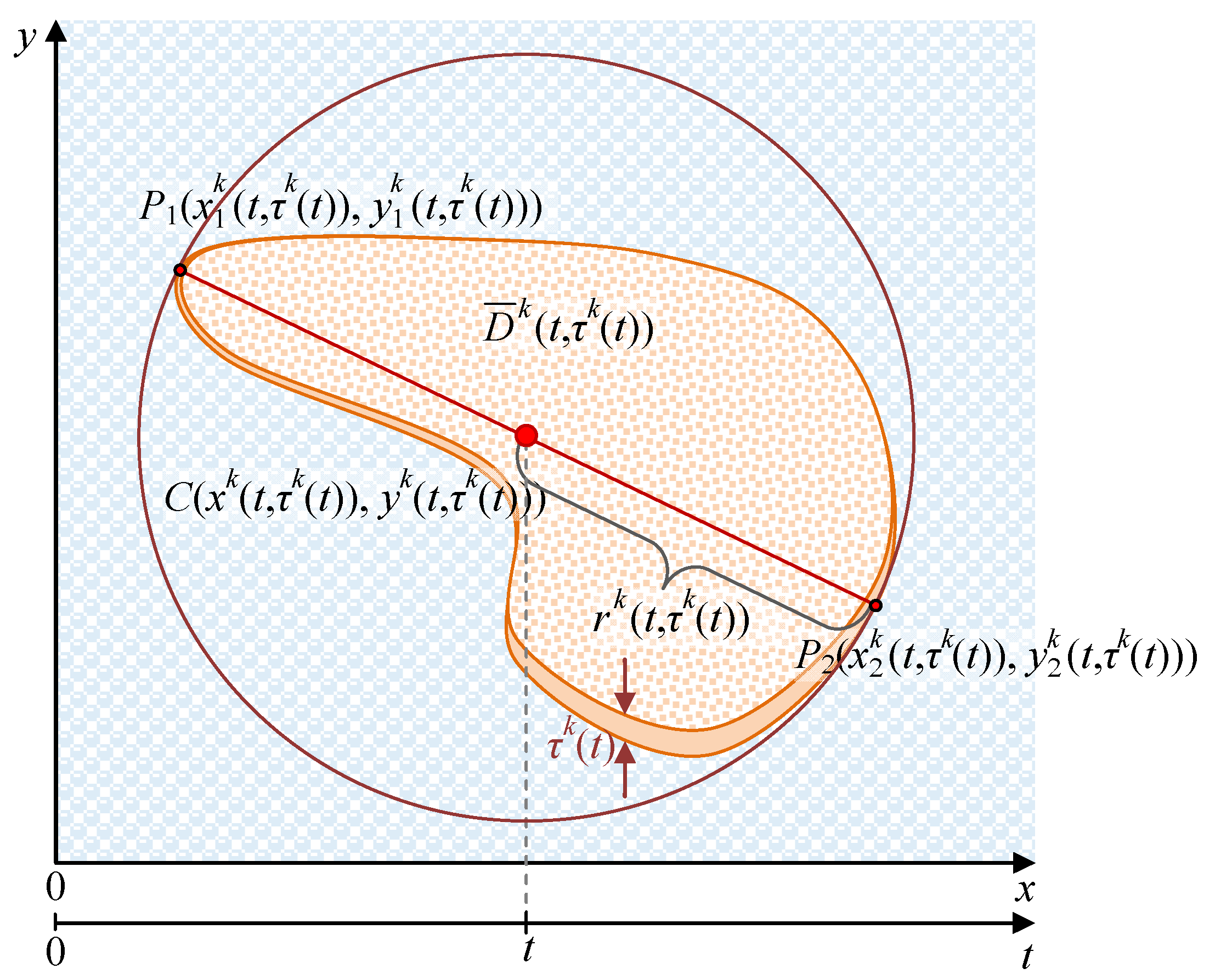
In this paper, we introduce a novel approach and assume that the oil slick thickness τ is changeable, i.e., τ = τk(t), in each hydro-meteorological state k and for t ∈ ⟨0, T⟩. Such an approach seems reasonable as the oil slick becomes thinner over time on the open sea [4]. Therefore, for the fixed oil slick domain k(t,τk(t)), k ∈ {1, 2, …, m}, t ∈ ⟨0, T⟩, we have
where P1(, ) and P2(, ) are the most distant points of the slick domain and C(xk(t,τk(t)), yk(t,τk(t))), as defined by Equation (10), is the central point (depicted in Figure 3). The radius is given by

Figure 3.
Graphical interpretation of the slick domain central point.
Further, for each fixed state k, k = 1, 2, …, m, of the process A(t) and time t, we define a two-dimensional stochastic process as follows:
where {Xk, ⟨0, T⟩ ℝ}, {Yk, ⟨0, T⟩ ℝ}, i.e.,
with values taken from a set of real numbers.
{Xk(t,τk(t)), Yk(t,τk(t)), t ∈ ⟨0, T⟩},
We deterministically set the central point of the oil slick domain, the oil release start point, as (0,0), and t = 0 at the moment of discharge, i.e.,
(Xk(0,0), Yk(0,0)) = (0,0).
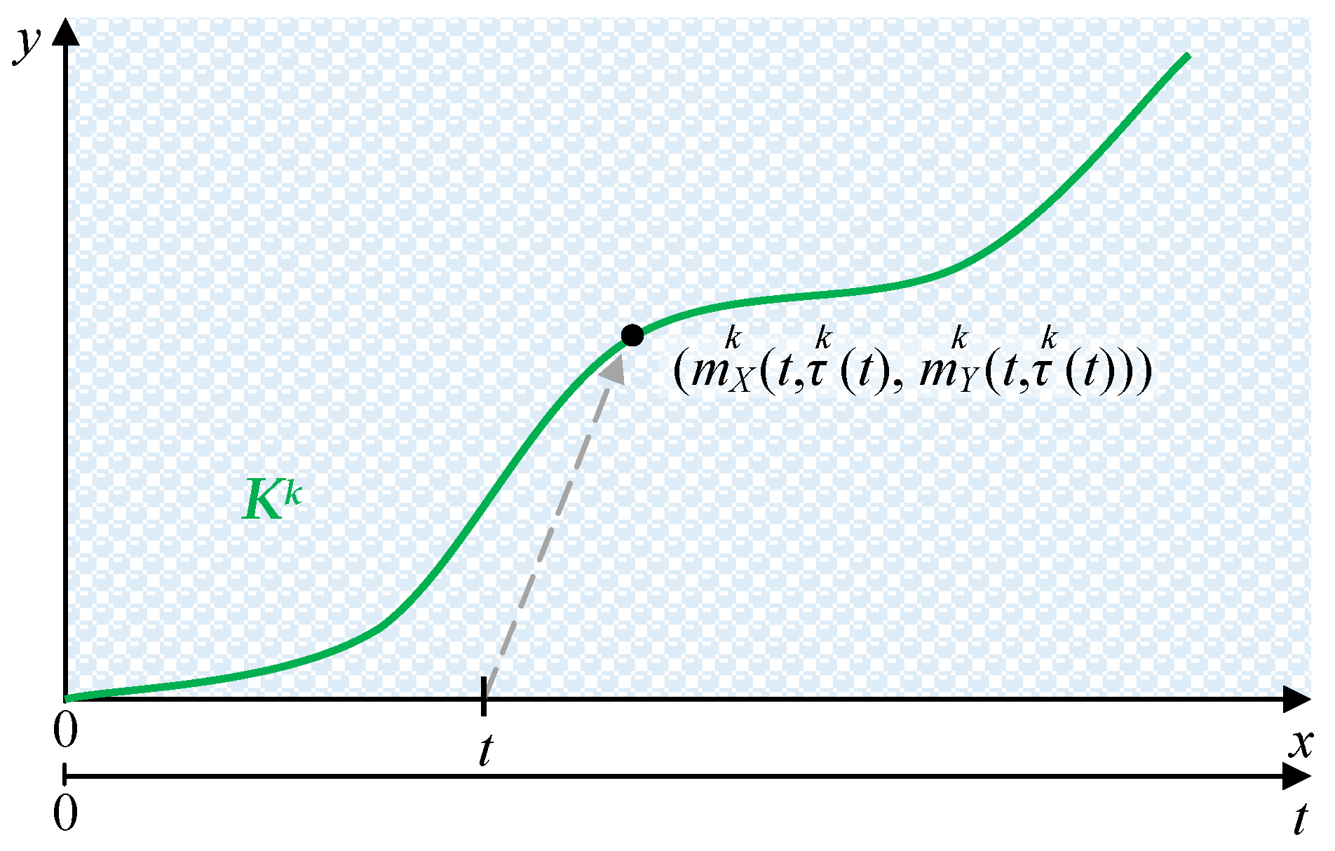
After some time, the central point starts its drift along a curve called a drift curve. In a further analysis, we assume that the processes given in Equation (14) for k ∈ {1, 2, …, m}, t ∈ (0, T⟩, are normal, with the expected values, standard deviations and correlation coefficients varying in time as follows:
i.e., with joint density functions:
where
Thus, the points given by (17), create a curve Kk (Figure 4) represented parametrically by
where τk(t), k ∈ {1, 2, …, m}, is the thickness of oil layer in a hydro-meteorological state at the moving central point.

Figure 4.
Central point drift trend.
3.3. Modelling Oil Slick Horizontal Movement and Dispersion
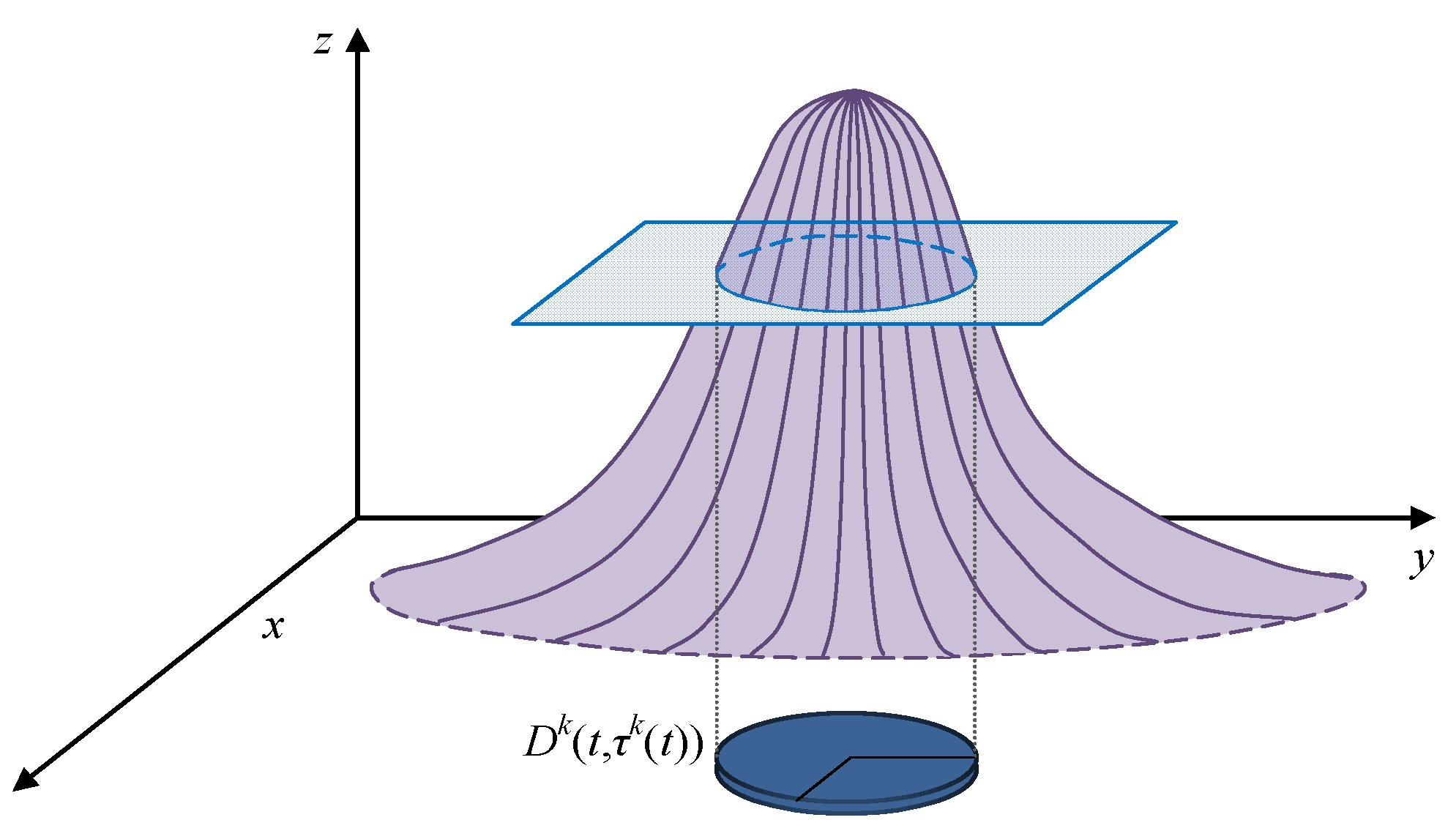
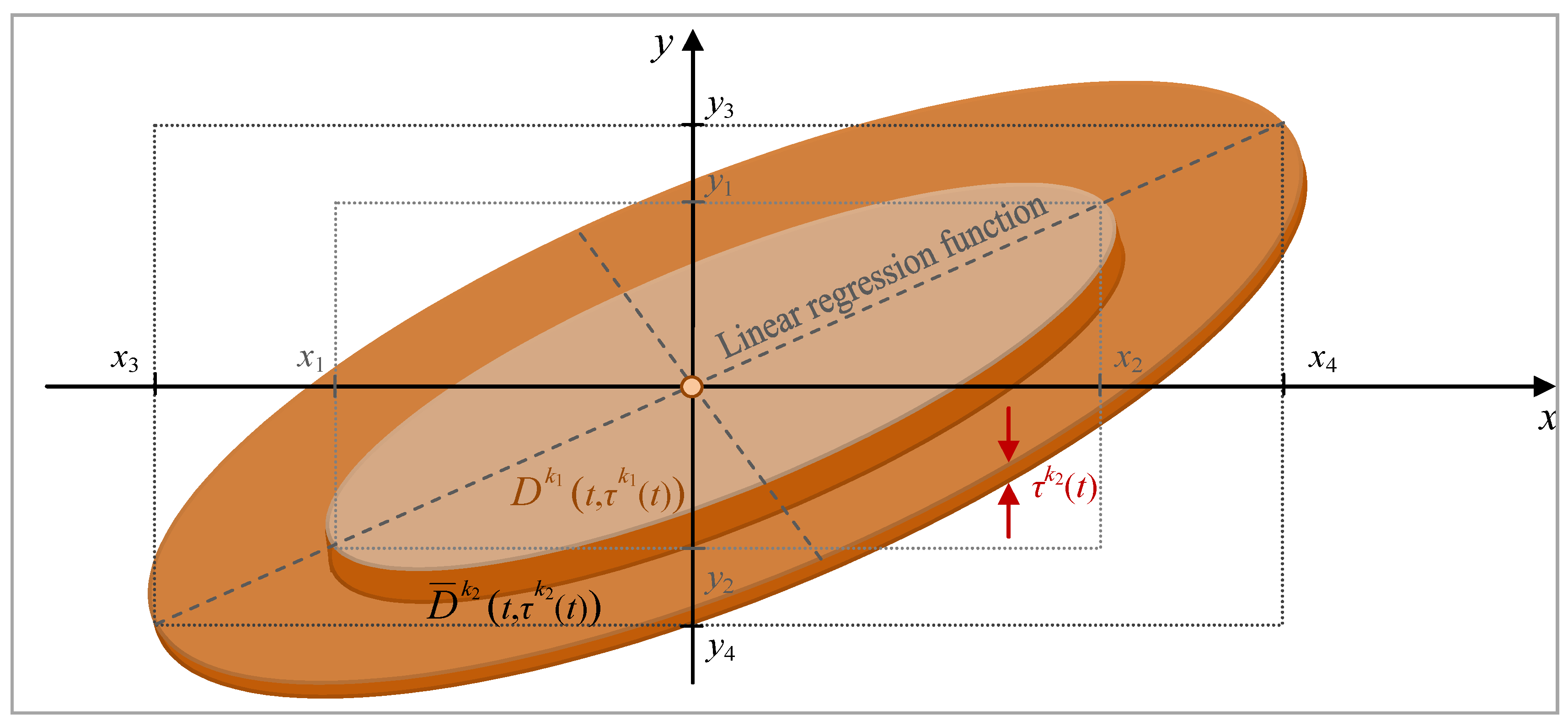
Assuming that the experiment takes place in the time interval ⟨0,T⟩, we are interested in finding the oil slick domain Dk(t,τk(t)), k ∈ {1, 2, …, m}, t ∈ ⟨0,T⟩, such that its central point is placed in it with a fixed probability p (Figure 5). From [12] and considering function (20), we have
where
is the domain bounded by an ellipse which is the projection of the curve on the XY plane resulting from the intersection (Figure 6) of the density function surface
and considering (21) the plane
k ∈ {1, 2, …, m}, t ∈ ⟨0,T⟩.

Figure 5.
Oil slick domain Dk1(t,τk1(t)) at hydro-meteorological state k1 after time t = 1Δt.

Figure 6.
Domain Dk(t,τk(t)) of integration bounded by an ellipse.
Considering the above and the assumptions in Section 3.2, the definition of the central point given by (10) for each fixed state k, k ∈ {1, 2, …, m}, of the process A(t) and time t ∈ (0,T⟩, we define and depict in Figure 7 the oil slick domain after time t = 2Δt:
where
for k ∈ {1, 2, …, m}, t ∈ ⟨0,T⟩, and rk(t,τk(t)) is the radius of the oil slick domain. It can be seen that the ellipses are bigger and thinner in Figure 7 than in Figure 5.

Figure 7.
Oil slick domain k2(t,τk2(t)) at hydro-meteorological state k2 after time t = 2Δt.
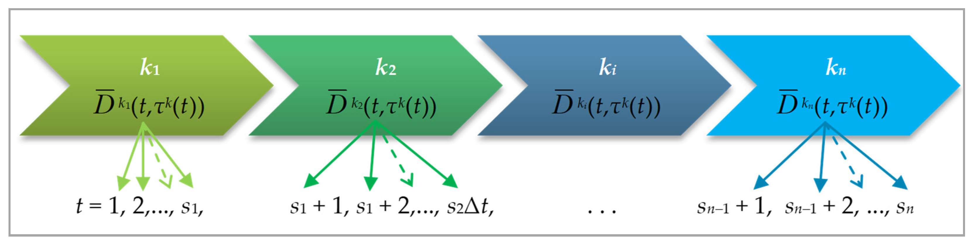
Consequently, we can assume the following:
- Varying hydro-meteorological factors that change at random times;
- Any quantity of hydro-meteorological factors considered in the model;
- The statesof the hydro-meteorological process A(t), taken in successive order;k1, k2, …, kn+1, where ki ∈ {1, 2, …, m}, i = 1, 2, …, n + 1,
- A fixed step of time ∆t;
- A changeable oil layer thickness τk(t) in each hydro-meteorological state;
- A number of steps si, i = 1, 2, …, n + 1;
- The time seriesin the process A(t)’s states.t = 1Δt, 2Δt, …, s1Δt, (s1 + 1)Δt, (s1 + 2)Δt, …, s2Δt, …,
(si−1 + 1)Δt, (si−1 + 2)Δt, …, siΔt, …, sn−1Δt, (sn−1 + 1)Δt, (sn−1 + 2)Δt, …, snΔt,
These assumptions allow for an enhanced prediction of how oil drifts and disperse over time.
The above figures (Figure 5 and Figure 7) depict the oil slick domains Dk1(t,τk1(t)) and k2(t,τk2(t)) in hydro-meteorological states k1 and k2 after time t = 1Δt and 2Δt. The points xι and yι, for ι = 1,2,3,4 are as follows:
where c exists in (27) and (28) and is equal to +/− p ∈ ⟨0,1⟩, and the linear regression function is
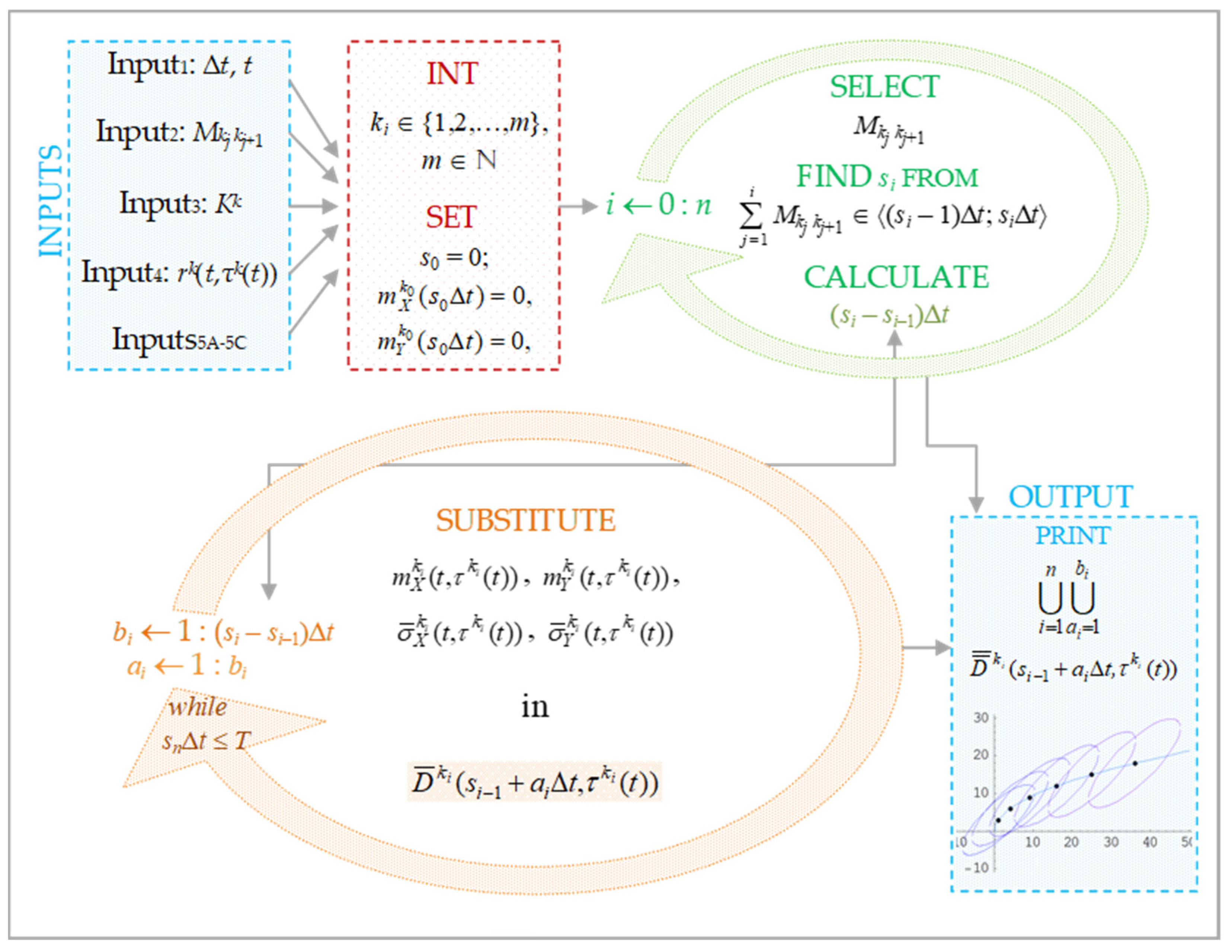
3.4. Procedure to Forecast the Horizontal Movement and Dispersion of an Oil Slick
Taking into account the above considerations, we can construct a prediction procedure for the surface movement and dispersion of an oil slick. The input parameters derived in the previous sections are as follows:
- Input1: step of time ∆t; time t, t ∈ (0,T⟩;
- Input2: mean values Mkjkj+1, defined by (7) and (8) in different hydro-meteorological states;
- Input3: oil spill central point drift trend Kk, given by (23);
- Input4: radius rk(t,τk(t)) dependent over time, given by (13);
- Input5A: expected values (t,τk(t)), (t,τk(t)), given by (17);
- Input5B: standard deviations (t,τk(t)), (t,τk(t)), given by (18);
- Input5C: correlation coefficient (t,τk(t)), given by (19).
Next, we may fix the states (32) as integers from a set {1, 2, …, m}, m ∈ ℕ, and set initial values of parameters. The new mean value from Input2 can be found after checking the boundaries of the range
((si−1 + 1)∆t, si∆t⟩, i = 1, 2, …, n + 1.
The output is represented as a domain consisting of the sum of the elliptical sub-domains (28) in the successive intervals (43) in the hydro-meteorological state ki, i = 1, 2, …, n + 1, with the appropriately substituted parameters (17), (30), and (31):
where bi := 1: (si − si−1)∆t and ai := 1: bi, i = 1, 2, …, n.
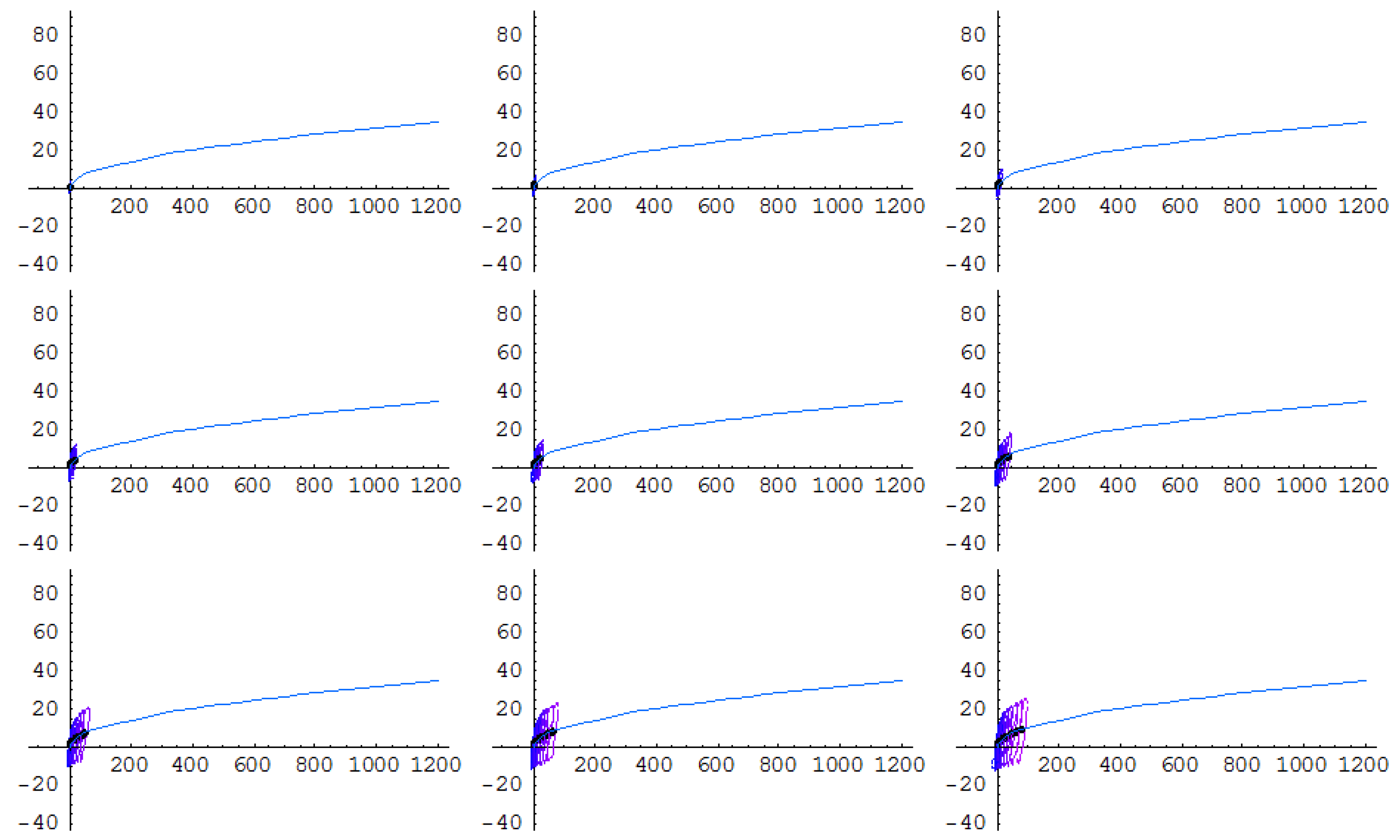
Further, considering the above, we receive the following sequence of oil spill domains (Figure 8), where si, i = 1, 2, …, n, are natural numbers.

Figure 8.
A graphical representation of a sequence of oil spill domains in a time series.
Figure 9 visualises an expanded procedure determining the oil slick’s horizontal movement and dispersion influenced by varying hydro-meteorological conditions and the thickness of the oil spill layer.

Figure 9.
The procedure of forecasting an oil slick’s horizontal movement and dispersion.
In the following section, the application of the procedure and the results are presented specifically for the Bornholm Basin in the Baltic Sea area.
4. Application and Results
4.1. The Bornholm Basin in the Baltic Sea
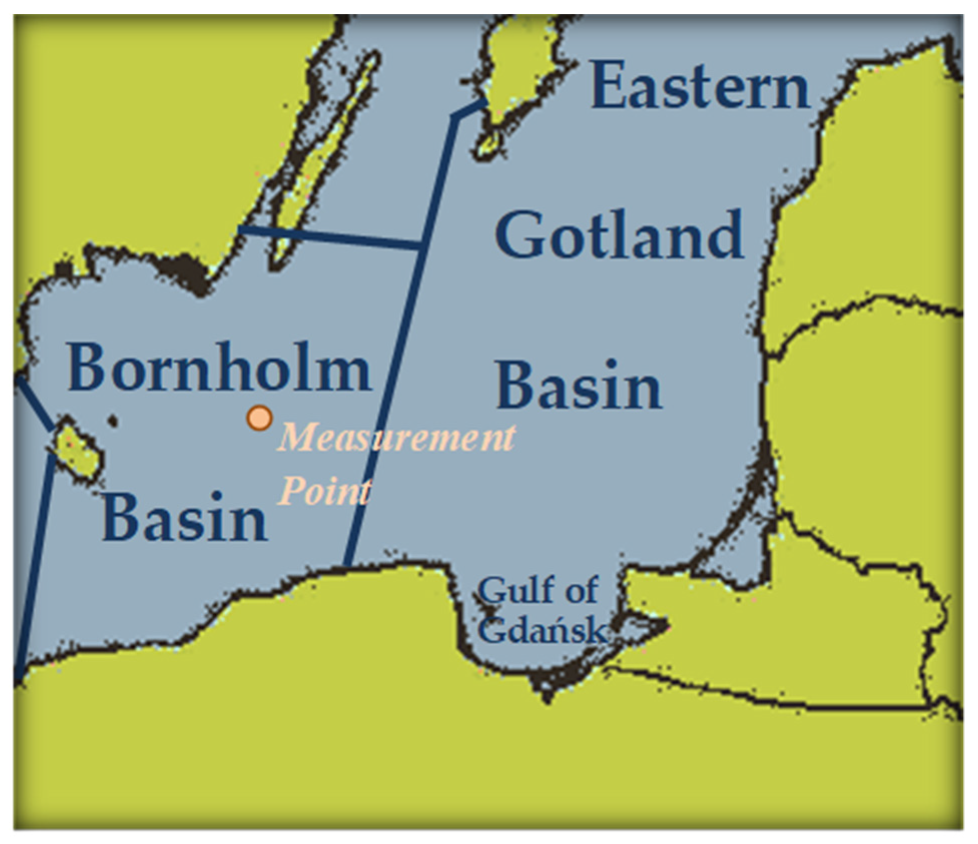
The selection of the Bornholm Basin in the Baltic Sea for illustrating the practical application of the proposed model from Section 3 stems from several factors. Primarily, the Baltic Sea was chosen due to the basin’s distinctive oceanographic attributes, its significance concerning oil spill risk, and the abundance of data sources available. Moreover, the Bornholm Basin specifically stands out due to its heightened maritime activity, characterised by heavy traffic and ship collisions, making it a pertinent case study for examining the implications of oil spills in such busy marine environments [23,24,25].
The measurement point illustrated in Figure 10 was considered. The data collected were joined from four points which were close to each other and tested successfully for uniformity, using procedures from [14,26].

Figure 10.
Measurement point located in the Bornholm Basin of the Baltic Sea.
4.2. Winds and Waves at the Bornholm Basin in the Baltic Sea
Information on winds and waves is essential for guaranteeing safe operation during maritime navigation. For many years, the Institute of Meteorology and Water Management at the National Research Institute in Poland has been involved in the monitoring of the Baltic Sea by undertaking measurements and research, consistently offering insights and expertise on data quality [27]. Additionally, rigorous validation and quality control measures were implemented to ensure the accuracy and integrity of the data employed for the analysis, further enhancing the robustness of the findings. Techniques such as data imputation, in which missing values are estimated based on existing data patterns or through statistical methods, were utilised to ensure continuity in the dataset. Collaborations with other data providers and institutions may also facilitate data exchange and supplementation to fill in gaps.
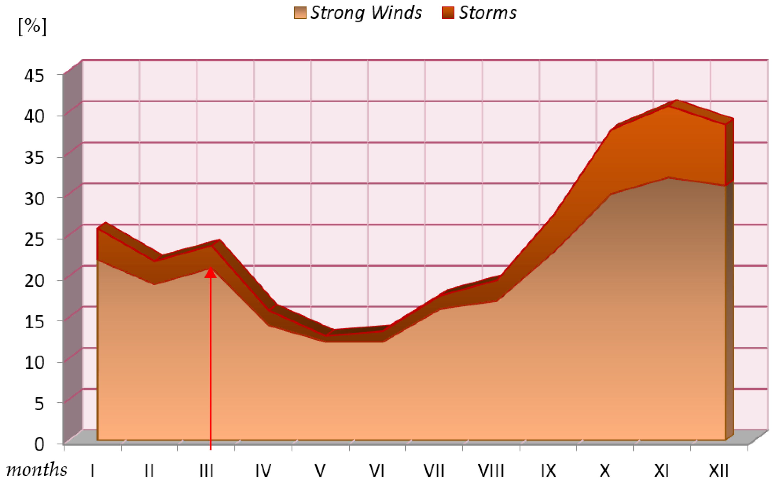
Winds and waves over the past few decades were analysed specifically for the Bornholm Basin in the Baltic Sea area. Statistical data (around 219,000 records) were analysed for months of March (GMU Safety Interactive Platform [28]) for six years of the experiment. March is the month in which the weather in the Bornholm Basin changes rapidly from noticeable, strong winds and storms to calm breezes [29]. This is why this is the major factor is in the investigation. South of the island of Bornholm is the centre of the highest frequency of strong breezes and storms. There are more than twice as many strong winds and more than three times as many storms as in most other coastal areas. The strongest winds (>33 m/s) seldom occurred in the considered area: they were recorded only in 1967 and 1999. Due to the extreme instability of the wind and wave direction in the spring, even nearby sites may experience various directions. The centre of intense wind and storm activity moves to the considered area in September. The frequency of high winds and storms increases significantly between August and October (Figure 11). It decreases noticeably between December and the beginning of January, and then it increases again between March and April.

Figure 11.
Average frequency of strong winds and storms for the south of Bornholm throughout a year [27].
The second notable parameter that the Institute suggested including is wave height. Significant waves of up to 14 m were noticed in the considered area. Higher waves could be noticed once every century. Low waves of up to 2 m predominate throughout the year in the considered area. Moderate waves of up to 5 m are frequently observed. Larger waves primarily happen in the winter. Although waves next to the Eastern Gotland Basin usually reach approximately 5 m, they can ascend to 8 m and, very rarely, they may even reach up to 10 m.
4.3. Hydro-Meteorological Input Data for the Model
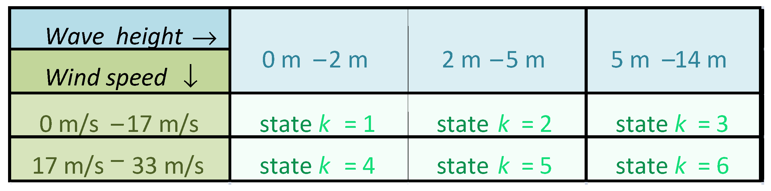
For the considered measurement point (Figure 10), wind speed and wave height data were collected from Meteorology and Water Management Institute under a copyright. The wind speed and wave height were divided into groups, and m = 6 states of the process of changing hydro-meteorological conditions were distinguished which can be represented in a matrix form illustrated in Figure 12.

Figure 12.
Fixed hydro-meteorological states.
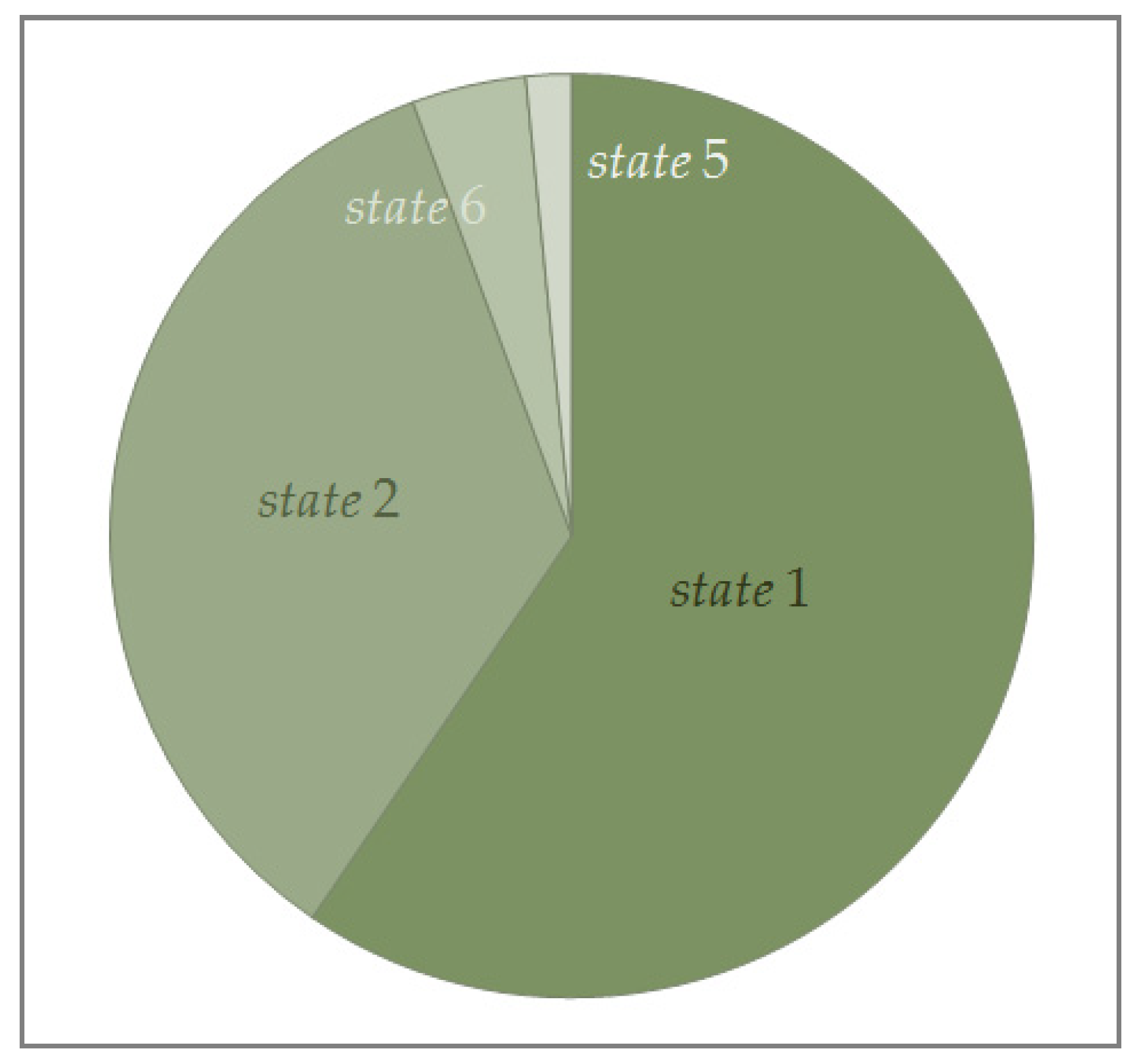
Then, the unknown parameters of the semi-Markov model of the hydro-meteorological change process were determined, i.e., the initial probabilities (Figure 13) and the probabilities of transitions between the process’ states were evaluated (Figure 14).

Figure 13.
The initial probabilities of the process.

Figure 14.
Graphs showing the probabilities of and transitions between the hydro-meteorological states.
Moreover, the hypotheses regarding the distribution functions Wkiki+1(t), ki ∈ {1, 2, …, 6}, given by Equations (5) and (6) were statistically verified using the methods from [14]. The mean values at different hydro-meteorological states ki, calculated according to (8) and measured in hours, are as follows:
4.4. Other Input Data for the Model
By repeatedly applying the procedure presented in Figure 9 in Section 3.4, we can forecast the oil slick domain that we are looking for. The data input into the model are as follows:
- The time step assumed to be ∆t = 1 h;
- The experiment time t, t ∈ ⟨0,48⟩, is represented by the time series t ∈ (si−1 + 1, si⟩, i = 1, 2, …, n;
- The mean values Mkiki+1, ki ∈ {1, 2, …, 6}, are taken from (48) in different hydro-meteorological states;
- The points (17) existing in Figure 4, forming a central point Kki given by (23), are represented by the equations , and τ ∈ (0, 1⟩;
- Standard deviations (18) are to be assumed time-dependent, = = 0.2·t + 0.1;
- The correlation coefficient (19) is = 0.8;
- Radii (13) are time-dependent, 0.5·t + 0.5.
In real practice, all the above parameters should be statistically identified using the methods given in [14]. The sequence of the hydro-meteorological change process’s states can be generated using a Monte Carlo simulation method, as in [12,13]. The oil slick thickness is assumed to be time-dependent and different in varying hydro-meteorological states.
Further, considering the above, Figure 8, and successively applying the procedure from Section 3.4, we obtain the sequence of oil spill domains that is presented in the next subsection.
4.5. The Results
The procedure was applied for the prediction of oil slick dispersion and horizontal movement in the Bornholm Basin area in the Baltic Sea (Figure 10). The iterative steps taken to draw the final result are depicted in Figure 15.

Figure 15.
The steps taken to determine final oil slick dispersion for the considered measurement point.
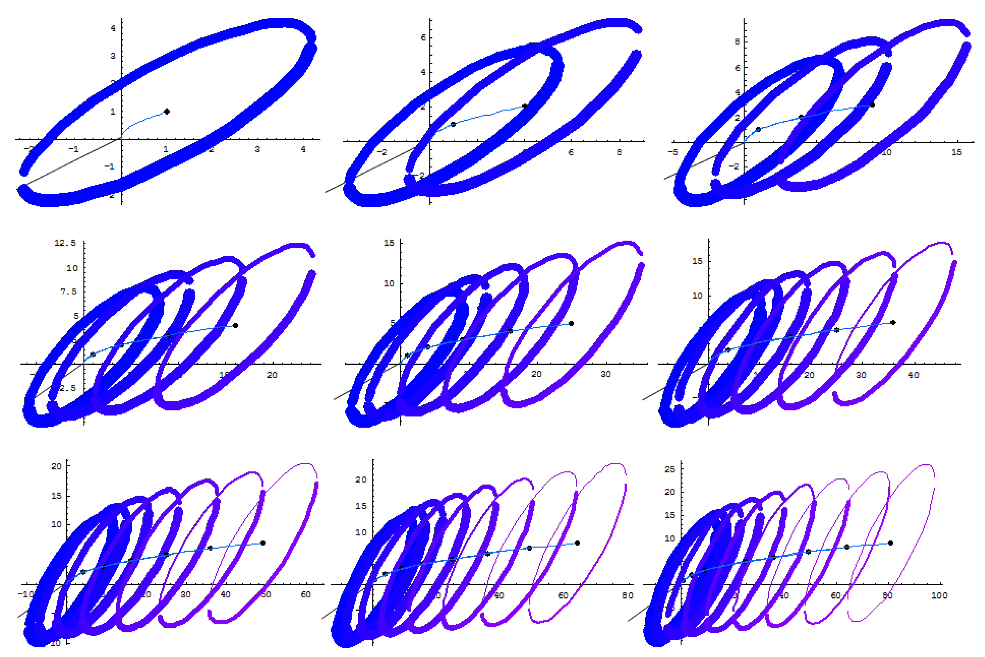
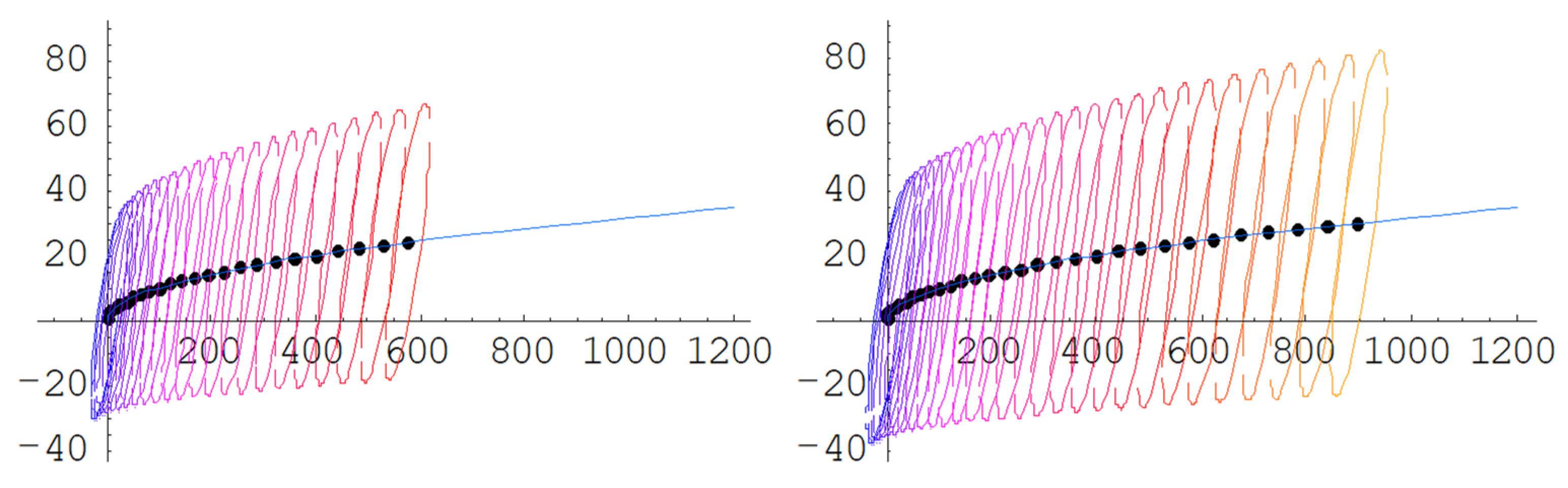
The results obtained are the sequences of oil spill domains for varying hydro-meteorological conditions two days after an oil leak. They are generated for selected t = {1 h, 2 h, 3 h, 4 h, 5 h, 6 h, 7 h, 8 h, 9 h, 24 h, 30 h, 48 h} and illustrated for the considered area, as shown in Figure 16, Figure 17, Figure 18 and Figure 19. The oil layer since the beginning of the spill starts from 1 mm thick, and after 9 h, it is around 0.2 mm thick.

Figure 16.
The sequence of oil spill domains in the considered measurement point area at the moments t = 1 h, 2 h, …, 9 h.

Figure 17.
The sequence of oil spill domains in the considered measurement point area at the moments 1 h, 2 h, …, 9 h at a different scale compared to Figure 16.

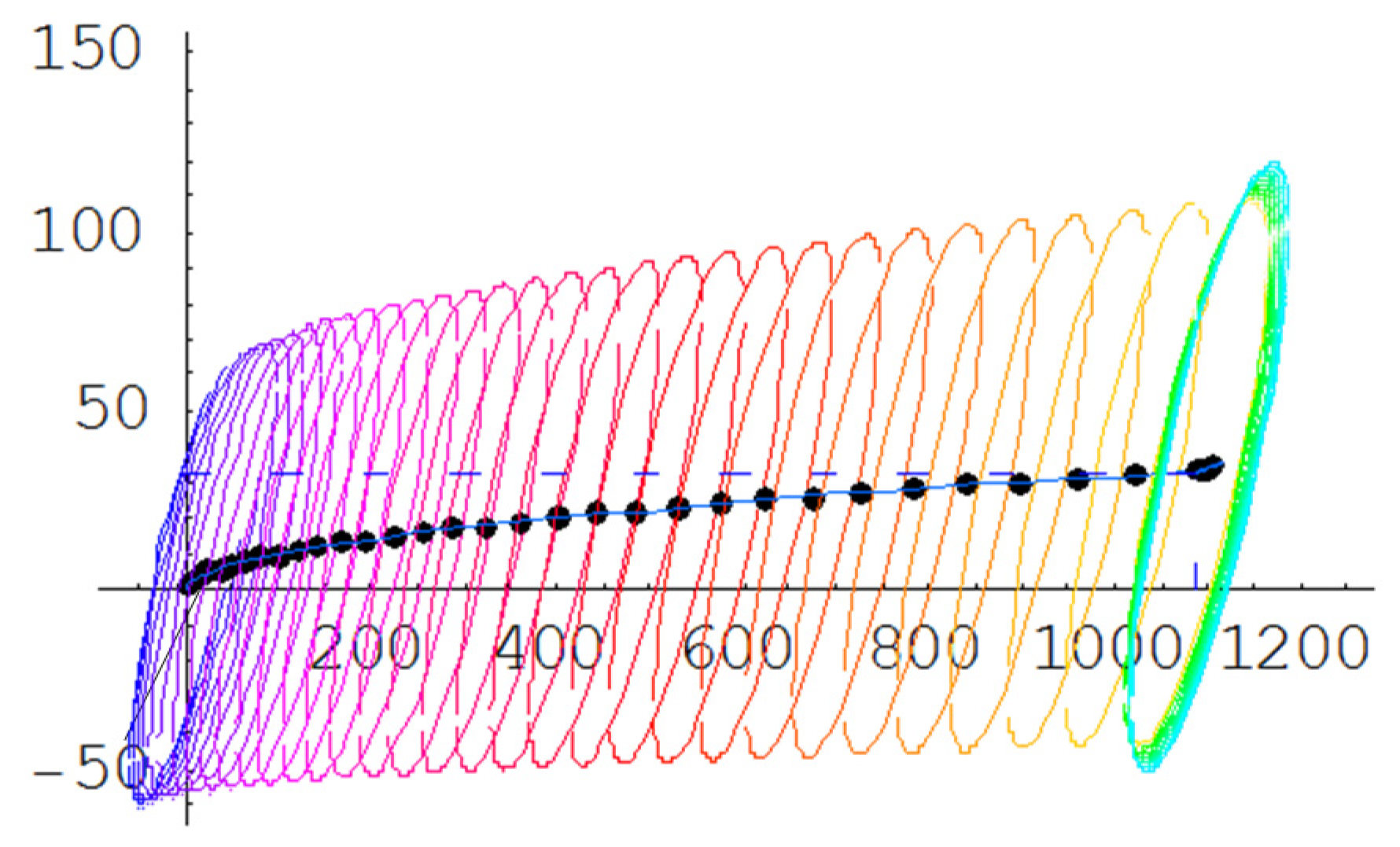
Figure 18.
The sequence of oil spill domains in the considered measurement point area at the moments t = 24 h, 30 h.

Figure 19.
The final oil spill domain in the considered measurement point area at the end of the experiment time.
In the experiment, the final representation of the oil spill domain consists of a combination of domains (Figure 19) in which actions of mitigating the oil release consequences can be carried out.
The results obtained in this study are as follows. When oil leaks, it begins as a single slick and quickly spreads across the surface of the sea (Figure 16). The initial thickness of an oil layer is set at 1 mm (1 h after the spill) and is influenced by hydro-meteorological conditions in such a way that it varies as the states change over time and the central point of each ellipse changes its position in a new trajectory as it is affected by the weather. The ellipses become bigger and thinner over time, as shown in the figures. After 24 h of the experiment, the oil is spread to almost 600 m in the considered water area of the Bornholm Basin, and it spreads to almost 900 m after 30 h (Figure 18). Figure 19 illustrates the final oil spill area composed of an elliptical combination of domains after 48 h of the experiment. The spread is more than 1200 m over the water area, considering the mild hydro-meteorological conditions (state 1 and state 2 in Figure 12).
For further predictions (longer than two days), the time can be increased and the procedure subsequently repeated until we reach a new value of T. However, after two days, oil slicks may cover unmanageable areas, and their thickness is too thin for skimmers to remove them efficiently. Thus, quick action is necessary to effectively clean up the contamination. The approach taken into consideration in this paper may help responders assess the extent of spills and mitigate the effects of harmful emissions in the case that the oil reach highly vulnerable ecosystems.
5. Discussion and Comments
In the paper, the Bornholm Basin region of the Baltic Sea was considered to illustrate the application of a model proposed in Section 3, taking into account the thickness of the oil spill layer and two important hydro-meteorological parameters: wind speed and wave height. These parameters were included in the study as per the suggestion of a National Research Institute of Poland, the Institute of Meteorology and Water Management. The model allows for the consideration of more than two hydro-meteorological factors, as assumed in Section 3.3. The states of the process can then be defined similarly to Figure 12 by extending the table and making the experiment a bit more complicated.
This study’s obtained results are preliminary results in the forecasting of oil slick movement and spreading as some of the input parameters in Section 4.3 were arbitrarily assumed. This simplification may not fully capture the complexity of real-world scenarios, potentially leading to oversights or underestimations. In real-life situations, their statistical identification is necessary, which can be achieved using methods from [30]. To validate the results, practical applications of the developed model, after performing scientific experiments and obtaining suitable statistical data, can be performed for different water areas. The author aims to conduct a practical scientific experiment in different water areas of the Baltic Sea with the intention of statistically identifying the unknown parameters of the proposed model. However, this will consume a significant amount of time and financial resources, especially if it is performed for different kinds of spills and includes the physical characteristics of oil and other processes, such as evaporation, sedimentation, and dispersion as well. Taking more variables as input data or changing the considered variables can allow for a more comprehensive approach.
The emphasis on a varying oil layer thickness is essential because it directly impacts the severity of environmental damage and the effectiveness of cleanup efforts. Unlike the physical characteristics of oil, which remain relatively constant once a spill occurs, the thickness of the oil layer can fluctuate over time due to factors like weather conditions, hydrodynamic conditions, and cleanup operations. Then, specific measures that could be implemented to improve oil spill mitigation efforts can be suggested. Thicker oil layers may require more intensive cleanup efforts, including mechanical removal or dispersant application, whereas thinner layers might be effectively addressed through natural dispersion or bioremediation.
Further research is intended to be related to methods of identifying the exact location of a spill area and ways to reach it quickly. With more accuracy, the model may be improved to offer a useful depiction of reality. The procedure can be developed by computing the average oil slick domain by repeating the experiment several times. The ultimate thickness is suggested to depend on a wider range of variables to ensure the greatest precision and correspondence to reality as possible. Moreover, this stochastically based model can be developed to provide a helpful reflection of reality with greater precision by gradually incorporating additional parameters. For a comprehensive understanding, factors such as the type of oil, degradation rate, and other relevant variables can be integrated into the model one at a time. This incremental approach allows for a deeper analysis of how each parameter affects the dynamics of an oil spill. The insights gained from this study can be used to predict oil spill trajectories in other sea water areas with similar conditions. Moreover, the successful completion of uniformity testing and the integration of the realisations of conditional sojourn times from several experiments or datasets can be performed. The final impact of this research should be a model for the rapid calculation of the situation at sea and consequence mitigation.
6. Conclusions
The application of the presented stochastically based model was described to support decision making in oil spill response. This approach is proposed to make modelling oil releases at sea in real time possible and, consequently, to make prevention and mitigation actions more effective. The complexity of the problem makes it challenging to predict the exact spread of an oil spill, and probabilistic modelling provides a useful framework for capturing this uncertainty. However, the rate at which an oil slick dissipates can vary depending on hydro-meteorological conditions and the oil volume discharged, as well as the other factors not considered in this paper, like the presence of cleanup efforts and the type of oil and its physical properties and behaviour. Even if the real oil trajectories are a bit different from those determined by the proposed methods, they can still identify the hazardous area and make a significant contribution to the oil spill investigation.
Funding
This research was funded from the statutory activities of Gdynia Maritime University, grant number WN/PI/2024/03: “The influence of the oil layer thickness and the hydro-meteorological changes process on the movement of oil spills at sea”.
Data Availability Statement
The data presented in this study are available on request from the author, excluding some data protected by copyright.
Conflicts of Interest
The author declares no conflicts of interest.
References
- Bogalecka, M. Consequences of maritime critical infrastructure accidents with chemical releases. Int. J. Mar. Navig. Saf. Sea Transp. 2019, 13, 771–779. [Google Scholar] [CrossRef]
- Cordes, E.E.; Jones, D.O.B.; Schlacher, T.A.; Amon, D.J.; Bernardino, A.F.; Brooke, S.; Carney, R.; DeLeo, D.M.; Dunlop, K.M.; Escobar-Briones, E.G.; et al. Environmental impacts of the deep-water oil and gas industry: A review to guide management strategies. Front. Environ. Sci. 2016, 4, 58. [Google Scholar] [CrossRef]
- Eckroth, J.R.; Madsen, M.M.; Hoell, E. Dynamic modeling of oil spill cleanup operations. In Proceedings of the 38th AMOP Technical Seminar on Environmental Contamination and Response, Vancouver, BC, Canada, 2–4 June 2015; pp. 16–35. [Google Scholar]
- Fingas, M. Oil Spill Science and Technology, 2nd ed.; Elsevier: Amsterdam, The Netherlands, 2016. [Google Scholar]
- Huang, J.C. A review of the state-of-the-art of oil spill fate/behavior models. In Proceedings of the International Oil Spill Conference Proceedings, San Antonio, TX, USA, 28 February–3 March 1983; Volume 1983, pp. 313–322. [Google Scholar]
- Fernandes, R.; Necci, A.; Krausmann, E. Model(s) for the Dispersion of Hazardous Substances in Floodwaters for RAPID-N; EUR 30968 EN; Publications Office of the European Union: Luxembourg, 2022; ISBN 978-92-76-46707-6. [Google Scholar] [CrossRef]
- Keramea, P.; Spanoudaki, K.; Zodiatis, G.; Gikas, G.; Sylaios, G. Oil spill modeling: A critical review on current trends, perspectives and challenges. J. Mar. Sci. Eng. 2021, 9, 181. [Google Scholar] [CrossRef]
- Spaulding, M.L. A state-of-the-art review of oil spill trajectory and fate modeling. Oil Chem. Pollut. 1989, 4, 39–55. [Google Scholar] [CrossRef]
- Guo, W.; Wu, G.; Jiang, M.; Xu, T.; Yang, Z.; Xie, M.; Chen, X. A modified probabilistic oil spill model and its application to the Dalian New Port accident. Ocean. Eng. 2016, 121, 291–300. [Google Scholar] [CrossRef]
- Saçu, Ş.; Şen, O.; Erdik, T. A stochastic assessment for oil contamination probability: A case study of the Bosphorus. Ocean. Eng. 2021, 231, 109064. [Google Scholar] [CrossRef]
- Dąbrowska, E. Conception of oil spill trajectory modelling: Karlskrona seaport area as an investigative example. In Proceedings of the 2021 5th International Conference on System Reliability and Safety (ICSRS), Palermo, Italy, 24–26 November 2021; Institute of Electrical and Electronics Engineers (IEEE): Piscataway, NJ, USA, 2021; pp. 307–311. [Google Scholar] [CrossRef]
- Dąbrowska, E. Oil discharge trajectory simulation at selected Baltic Sea waterway under variability of hydro-meteorological conditions. Water 2023, 15, 1957. [Google Scholar] [CrossRef]
- Dąbrowska, E.; Kołowrocki, K. Monte Carlo simulation approach to determination of oil spill domains at port and sea waters areas. TransNav Int. J. Mar. Navig. Saf. Sea Transp. 2020, 14, 59–64. [Google Scholar] [CrossRef]
- Kołowrocki, K.; Soszyńska-Budny, J. Reliability and Safety of Complex Technical Systems and Processes: Modeling—Identification—Prediction—Optimization, 1st ed.; Springer: London, UK, 2011. [Google Scholar]
- Pietrucha-Urbanik, K.; Rak, J. Water, resources, and resilience: Insights from Diverse Environmental Studies. Water 2023, 15, 3965. [Google Scholar] [CrossRef]
- Tchórzewska-Cieślak, B.; Piegdoń, I. Matrix analysis of risk of interruptions in water supply in terms of consumer safety. J. Konbin 2012, 24, 125–140. [Google Scholar] [CrossRef]
- Fingas, M. The challenges of remotely measuring oil slick thickness. Remote Sens. 2018, 10, 319. [Google Scholar] [CrossRef]
- Fingas, M. How to measure slick thickness (or not). In Proceedings of the 35th AMOP Technical Seminar on Environmental Contamination and Response, Vancouver, BC, Canada, 5–7 June 2012; pp. 617–652. [Google Scholar]
- Global Marine Oil Pollution Information Gateway. What Happens to Oil in the Water? Available online: http://oils.gpa.unep.org/facts/fate.htm (accessed on 1 February 2024).
- Bogalecka, M.; Kołowrocki, K. Minimization of critical infrastructure accident losses of chemical releases impacted by climate-weather change. In Proceedings of the 2018 IEEE International Conference on Industrial Engineering and Engineering Management (IEEM), Bangkok, Thailand, 16–19 December 2018; pp. 1657–1661. [Google Scholar] [CrossRef]
- Yuriy, D.; Dobrin, M. Oil spills weathering. Ann. Rev. Res. 2022, 8, 555730. [Google Scholar]
- Torbicki, M. Longtime Prediction of Climate-Weather Change Influence on Critical Infrastructure Safety and Resilience. In Proceedings of the 2018 IEEE International Conference on Industrial Engineering and Engineering Management (IEEM), Bangkok, Thailand, 16–19 December 2018; pp. 996–1000. [Google Scholar] [CrossRef]
- Bogalecka, M. Consequences of Maritime Critical Infrastructure Accidents. Environmental Impacts. Modeling—Identification—Prediction—Optimization—Mitigation; Elsevier: Amsterdam, The Netherlands, 2020. [Google Scholar] [CrossRef]
- Dobrzycka-Krahel, A.; Bogalecka, M. The Baltic Sea under Anthropopressure—The Sea of Paradoxes. Water 2022, 14, 3772. [Google Scholar] [CrossRef]
- Magryta-Mut, B. Modeling safety of port and maritime transportation systems. Sci. J. Marit. Univ. Szczec. 2023, 74, 65–74. [Google Scholar] [CrossRef]
- Dąbrowska, E.; Torbicki, M. Hydro-Meteorological Changes Forecast of Southern Baltic Sea. Water, 2024; under review. [Google Scholar]
- Jakusik, E. The Impact of Climate Change on the Characteristics of the Wave in the Southern Part of the Baltic Sea and Its Consequences for the Polish Coastal Zone. Ph.D. Thesis, IMGW-PIB, Marine Research Department, Warsaw, Poland, 2012. [Google Scholar]
- Gdynia Maritime University Safety Interactive Platform. Available online: http://gmu.safety.umg.edu.pl/ (accessed on 1 February 2024).
- Rutgersson, A.; Kjellström, E.; Haapala, J.; Stendel, M.; Danilovich, I.; Drews, M.; Jylhä, K.; Kujala, P.; Larsén, X.G.; Halsnæs, K.; et al. Natural hazards and extreme events in the Baltic Sea region. Earth Syst. Dyn. 2022, 13, 251–301. [Google Scholar] [CrossRef]
- Dąbrowska, E. Modelling oil spill layer thickness and hydro-meteorological conditions impacts on its domain movement at sea area. In Safety and Reliability of Systems and Processes, Summer Safety and Reliability Seminar; Krzysztof, K., Magdalena, B., Ewa, D., Beata, M.-M., Eds.; Gdynia Maritime University: Gdynia, Poland, 2022; pp. 51–64. [Google Scholar] [CrossRef]


Disclaimer/Publisher’s Note: The statements, opinions and data contained in all publications are solely those of the individual author(s) and contributor(s) and not of MDPI and/or the editor(s). MDPI and/or the editor(s) disclaim responsibility for any injury to people or property resulting from any ideas, methods, instructions or products referred to in the content. |
© 2024 by the author. Licensee MDPI, Basel, Switzerland. This article is an open access article distributed under the terms and conditions of the Creative Commons Attribution (CC BY) license (https://creativecommons.org/licenses/by/4.0/).