
Dynamics of River Flood Waves below Hydropower Dams and Their Relation to Natural Floods

Department of Earth, Environmental and Planetary Sciences, Washington University, St. Louis, MO 63130, USA
Water 2024, 16(8), 1099; https://doi.org/10.3390/w16081099
Submission received: 25 February 2024
/
Revised: 24 March 2024
/
Accepted: 9 April 2024
/
Published: 11 April 2024
(This article belongs to the Special Issue Research on Geological Hazards and Geological Environment Issues Related to Mine Water)
Abstract
:The dynamic behavior of flood waves on rivers is essential to flood prediction. Natural flood waves are complex due to tributary inputs, rainfall variations, and overbank flows, so this study examines hydropower dam releases, which are simpler to analyze because channel effects are isolated. Successive arrival times and heights of peaks along 9 rivers with multiple stream gauges downstream of hydroelectric dams show that flow peaks typically become exponentially lower and wider with distance. The propagation velocity of peaks increases with water depth and channel slope but decreases with downstream distance and greater channel tortuosity. A rich hierarchy of velocities was found. Hydropower pulses progress at or in slight excess of the theoretical celerity, which is faster than the propagation rate of average natural floods, which in turn exceeds the mean velocity of water in the channel, yet the water moves faster than the peaks of record floods. The progressive changes to the height, shape, and velocity of hydropower flow peaks are simulated by the first analytical solution to the convolution integral for a rectangular source pulse that is based on diffusion-advection theory. Available data support some widely held expectations while refuting others. An expanded definition of “water mining” is proposed.
1. Introduction
The dynamic behavior of flood waves on rivers is an essential element of flood prediction. Natural flood waves are driven by heavy rainfall, but tributaries, spatial and temporal variations in rainfall delivery, channel shape, storage details, and many other effects are also significant. Much effort has been made to develop flood routing methods (e.g., [1,2]), and complex algorithms are used to forecast the arrival times and heights of floods on many rivers [3].
Considering the societal and economic importance of flooding, the wealth of available data on real flood waves has been little used. Most available studies concern theoretical or modeling efforts that utilize complex equations, provide no closed-form analytical solutions, and make minimal comparisons of results to data. Ferrick [4] analyzed the Saint-Venant equations under a set of varying parameter proportions and concluded that most river flow pulses are shallow-water gravity waves that are little influenced by friction. Other studies use models such as HEC-RAS or Flow-3D to simulate discharge under different scenarios, with most effort being centered on dam failures (e.g., [5,6,7]). As pointed out by Criss and Hofmeister [8], the number of free and poorly constrained parameters in many hydrologic models exceeds the number of observable quantities that are demonstrably simulated, in which case their predictions are underconstrained.
An exception is provided by the basic forms of the diffusion and diffusion-advection equations, which incorporate an absolute minimum of adjustable constants, have found broad application in the physical sciences (e.g., [9]), and have been widely used to investigate flood waves (e.g., [10,11,12,13,14]). The compact, fundamental solutions to these equations bear greater fidelity to the mathematical shape of real hydrographs than do other functions and simulations, and have served as effective transfer functions in rainfall-runoff simulations [15,16].
A key descriptor of river wave dynamics is the observed propagation velocity of the flood peak. Standard theory shows that the speed, or celerity c, of flood waves should be about 50% faster than the average velocity Vavg of water in the channel [2]. As is also well known, the theoretical celerity of “shallow water waves” increases with the square root of water depth [17,18]. Field studies are essential to confirm the applicability of these results to rivers, but they are far fewer than modeling efforts. The pioneering study of Faye and Cherry [19] to define river wave behavior deserves special mention, as they utilized data from multiple gauging stations along a river to investigate pulse behavior, although only a few days of data were investigated. Moody [20] used data from multiple gauging stations to define the propagation rate of the huge 1993 flood on the Mississippi River. Data show that the wave speed on rivers depends in a complex way on discharge, particularly on whether the flow remains within banks or extends over the floodplain [21,22].
The behavior of flow pulses generated at hydropower dams is much less complex than that of natural flood waves triggered by rainfall. Hydropower dam releases have simple shapes, are generated at a single site, and exclude overbank flows. It follows that these man-made pulses allow the dynamic behavior of in-channel flows to be isolated and understood, which behavior is an important part of the complex behavior of natural floods.
Scheduled hydropower pulses are also of environmental and management interest, as they can be sudden and large and, at many sites, are preceded by warning sirens [23]. Although the term “water mining” is conventionally used to describe groundwater extraction, the releases of hydroelectric dams also constitute water mining, as they are used to extract the potential energy from impounded waters. Moreover, like mine waters, the released waters are environmentally problematic, as they are abnormally cold and deoxygenated, commonly contain excess nitrate and other contaminants, and have high erosive power because of their high velocity and low content of suspended sediment, all due to their protracted storage in the upstream reservoir [24,25,26].
This paper provides the most comprehensive analysis yet available of the velocity and attenuation of in-channel flow pulses generated by hydropower dams. Several years of data are analyzed from 29 river gauges located at increasing distances below dams on 9 rivers that span the United States (Figure 1a) and exhibit a large range of sizes, depths, and channel slopes. Data are available for water levels at 15 min intervals [27], permitting the arrival times and heights of flow peaks to be accurately determined at successive sites. Many dynamic behaviors are revealed by investigating pulse behavior along individual rivers, and others are revealed by comparing data from multiple rivers. This study also provides the first closed-form analytical solutions to the convolution integral for a rectangular flow source, which represents a very common pattern for dam releases. This solution predicts the evolving shapes and attenuation of a moving hydropower pulse and links the functional relationships among master variables. This solution embodies only familiar functions, so it can be easily used in ordinary spreadsheet programs, and direct analogues could be applied to diverse problems in the physical sciences, such as the behavior of dye tracers or the fate of contaminant pulses in streams. Finally, the comparison of natural river floods to hydropower pulses reveals important similarities and differences.
2. Methods
The propagation velocity of flow peaks was determined by first identifying rivers that are monitored by several stream gauges located at increasing distances below a hydropower dam (Figure 1). Adequate archives [27] of water levels (h) and commonly also discharge (Q) at 15 min intervals were found for several such rivers. Distances between sites (∆x values) are also needed to determine the propagation rates of hydropower peaks between two sites, here termed Vhp. These inter-site distances are easily determined by subtracting published stream gauge locations in “river miles” along the channel, but where such are not available, they were measured using satellite images and standard GIS tools. The average slope of the channel bottom between any two sites was determined by taking the reported elevations for gauge zero, corrected for the local stage (So) of the bottom as determined by method 3 of Criss and Nelson [31], divided by the thalweg distance between the sites.
A simple method was devised to determine the average delay of flow variations between two successive sites that can utilize all available data in a lengthy record of several years. First, a table was prepared with a column that represents a uniform time series (t values for 15 min intervals) plus two columns for the water levels recorded at the two sites. The water level h1 at site 1 was then plotted against level h2 at site 2, and the correlation coefficient (R2) of the linear regression was noted. Then, the stage record for the antecedent (upstream) site was delayed by a single, 15 min time step by inserting an empty row at the head of its column. Then, the graph was re-plotted, and the correlation coefficient was recalculated. Additional rows were added until the highest correlation coefficient was found, with the number of added rows indicating the “best” inter-site delay time. The overall best average value for Vhp was found by dividing the inter-site distance by this optimized delay time. Results for several rivers are provided in Table 1.

Table 1.
Characteristics of gauged sites below hydropower dams.
| River | Site * | Dist, km | Zero *, m MSL | Vhp m/s | “Vavg” m/s | Slope m/km | Tortuo-sity † | Time ‡ Const, d | So m | m † |
|---|---|---|---|---|---|---|---|---|---|---|
| Osage | 06926000 | 2.09 | 167.38 | 0.94 | 0.53 | 0.04 | 1.2 | |||
| “ | 06926080 | 24.62 | 164.83 | 1.65 | 1.07 | 0.11 | 1.63 | 1.37 | 0.07 | 1.9 |
| “ | 06926510 | 75.94 | 160.20 | 1.61 | 0.76 | 0.09 | 1.69 | 1.93 | 0.28 | |
| Salt | 05507800 | 0.80 | 152.40 | 0.76 | 0.49 | 0.36 | ||||
| “ | 05508000 | 28.96 | 145.40 | 1.21 | 0.72 | 0.25 | 1.90 | 0.69 | 0.44 | 1.3 |
| Sac | 06919000 | 1.21 | 231.25 | 0.76 | 1.2 | |||||
| “ | 06919020 | 10.78 | 228.66 | 1.07 | 0.63 | 0.27 | 2.21 | 0.31 | 1.26 | 1.5 |
| “ | 06919900 | 41.83 | 219.79 | 1.39 | 0.80 | 0.28 | 2.07 | 0.65 | 1.23 | |
| Cumberland | 03414000 | 2.41 | 164.62 | 1.07 | 0.30 | 1.4 | ||||
| “ | 03414100 | 54.22 | 152.28 | 1.52 | 1.03 | 0.12 | 2.27 | 1.69 | 6.52 | 2.2 |
| “ | 03417500 | 128.4 | 149.03 | 1.74 | 0.98 | 0.13 | 2.55 | 0.31 | ||
| Allegheny | 03012550 | 0.80 | 363.57 | 0.85 | 2.88 | 2.16 | ||||
| “ | 03015310 | 14.0 | 356.01 | 2.64 | 2.82 | 0.73 | 1.15 | 2.22 | 0.13 | |
| “ | 03016000 | 63.07 | 322.91 | 2.99 | 1.03 | 0.67 | 1.32 | 3.75 | 0.53 | 2.1 |
| Colorado | 09380000 | 25.74 | 946.76 | 0.98 | 1.04 | 0.67 | ||||
| “ | 09402500 | 166.4 | 737.22 | 1.97 | 1.56 | 1.52 | 1.47 | 1.62 | −2.8 | 2.5 |
| “ | 09404200 | 387.6 | 408.43 | 2.32 | 1.48 | 1.42 | 1.83 | 1.73 | 12.4 | |
| Kootenai | 12301933 | 1.13 | 640.08 | 1.12 | 2.77 | 4.12 | ||||
| “ | 12305000 | 81.25 | 547.04 | 2.77 | 2.15 | 1.19 | 1.36 | 3.08 | 1.83 | 1.7 |
| “ | 12308000 | 100.6 | 518.16 | 2.37 | 1.34 | 0.52 | 1.34 | 3.51 | 20.7 | |
| Snake | 13290450 | 1.45 | 437.39 | 2.15 | 0.77 | 16.8 | 1.9 | |||
| “ | 13317660 | 115.8 | 259.08 | 2.82 | 1.65 | 1.71 | 1.35 | 1.67 | −0.5 | |
| “ | 13334300 | 129.5 | 245.88 | 3.04 | 2.23 | 0.93 | 1.20 | 2.09 | −0.1 | 2.1 |
| Missouri # | 06467500 | 8.21 | 347.53 | 1.12 | ||||||
| “ | 06478526 | 57.44 | 335.28 | 1.21 | 1.07 | 0.21 | ||||
| “ | 06486000 | 126.6 | 322.30 | 1.16 | 1.70 | 0.21 | −2.0 | |||
| “ | 06601200 | 192.9 | 308.02 | 1.48 | 1.74 | 0.19 | 1.56 | |||
| “ | 06610000 | 313.8 | 289.25 | 1.30 | 1.79 | 0.16 | 0.51 | |||
| 06807000 | 399.5 | 276.03 | 1.70 | 1.97 | 0.16 | 0.45 |
Note(s): * Site number and gauge zero from ref. [27]; † Dimensionless. Tortuosity is the channel path length divided by the straight-line distance; m is defined in Equation (3); ‡ Calculated using Equation (2) of [32], typically using all 15 min data in a 4-year interval; # For the Missouri River sites, the Vhp values represent only two weeks of data.
For the Osage River (Figure 1b), a detailed study was made of the successive arrival times and heights of individual flow pulses at three gauges. A preliminary list of pulse events was generated using the standard capabilities of spreadsheet programs to identify daily flow peaks above an arbitrary minimum stage of 0.75 m. This was followed by a tedious visual inspection of the computer generated list, which was required to eliminate events where multiple peaks occurred in short succession and then mutually interfered, where data were missing at critical intervals, or where downstream sites had much higher volumes of water than sites upstream, indicating unwanted inputs of rainfall or variable tributary inflows. A total of 494 isolated flow peaks were identified that could be reliably tracked downstream and occurred between January 2018 and November 2023. Results for this group are graphically analyzed below.
Different velocities are distinguished below and are abbreviated as follows: celerity (c), average water velocity (Vavg), and the propagation rates of flow peaks associated with hydropower pulses (Vhp), normal, rainfall-driven floods (Vnflood), record natural floods (Vrflood), and generic flow peaks (Vpk). All are theoretically and observationally different, and all are relevant to the flood phenomenon.
3. Theoretical Predictions
3.1. Standard Theory
Theoretical studies of water waves are varied and extensive, so only a few basic results are presented here. Because the effective wavelength of flood waves and hydropower pulses on rivers is much greater than the water depth, the shallow water condition applies. In this case, the celerity, also called the phase velocity or simply the “wave speed”, is as follows:
where g is gravitational acceleration, H is the water depth, and α is the slope, which is very flat for rivers, so cosα is very close to unity [17]. Equation (1) reduces to the familiar result for ocean waves [18], because both α and Vavg are zero. In contrast, most treatments of flood waves use a proportionality factor m to compare the celerity c with the average velocity Vavg of water flowing in the channel [2] as follows:
Values of m are typically predicted to be 1.5 ± 0.25, depending on channel shape and other assumptions. For example, Whitham [17] states that m is 3/2 if the Chezy equation is assumed and is 5/3 if Manning’s equation is assumed. Alternatively, reference [2] states that m is equal to the exponent in the power law as follows:
where Q is discharge, A is the area of the channel cross-section, and k and m are constants. The values for m in Table 1 were calculated from a graph of LogQ vs. Log A using available field data [27] and are provided only if the correlation coefficient of the plot exceeds 0.9. Values of m must be greater than unity for any channel because both Vavg and A increase with water level. For a triangular weir, m equals 1.25, whereas m is about 1.6 for a typical river [33]. In all these cases, the evident prediction is that c > Vavg.
Empirical tests of the above equations are made below, and these show that not all are supported for rivers. At the outset, note that Equations (1) and (2) are functionally compatible only if Vavg is proportional to the square root of gH cosα. Also note that Equation (1) predicts that celerity must exceed 3 m/s for any broad wave if the water depth exceeds ~0.9 m, given the magnitude of g.
3.2. Simple Diffusion
Flood waves do not move down river channels by diffusion alone, but because diffusion contributes to this process, it is useful to consider the consequences of this endmember mechanism as a starting point. The one-dimensional diffusion equation expressed for hydraulic head h is as follows:
where κ is the hydraulic diffusivity (e.g., [34]). Criss and Winston [35] combined this equation with Darcy’s law to obtain a solution for discharge as a function of time that is generated by a sharp source pulse in the head (delta function) as follows:
where Qpk is the peak flow at the site, which occurs at time 2b/3, where b is the time constant, which in turn equals the quantity x2/4κ. Equation (5) was originally derived to simulate the diffusive delivery of rainfall runoff to the river channel or spring orifice and not the flow of water down the channel, although it provides insight on the latter process. For that case, the apparent velocity of a sharp flow peak between two sites located at distances x2 and x1 below the source that have distinct time constants of b2 and b1 is as follows:
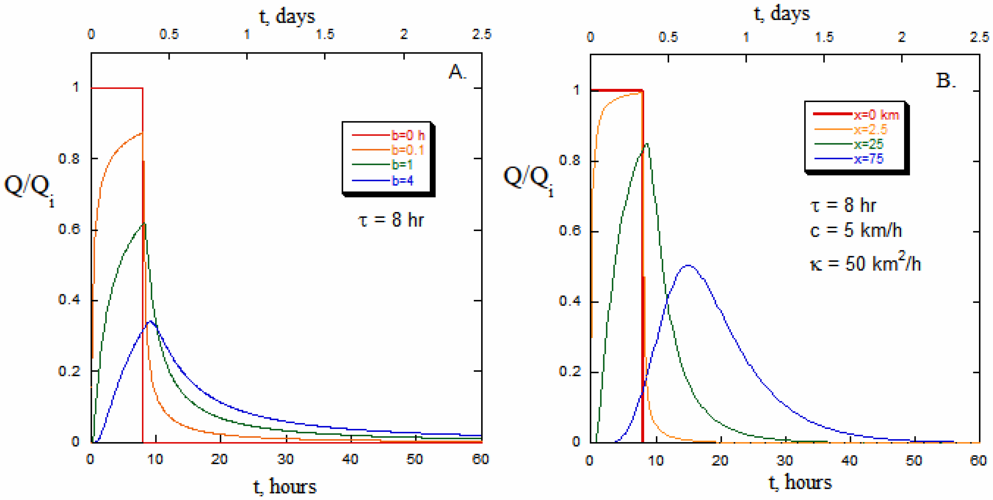
For unimpounded Missouri river basins, b in days is empirically proportional to 0.0135 times the square root of basin area in square km [36]. The rough estimate for peak velocity approximates 1.5 times the reciprocal of this number, or about 100 km/d. Again, because Equation (5) was developed to simulate the diffusive delivery of runoff and not the much faster flow of river water down the channel, the values for b that characterize river basins are much longer than those relevant to river channels, which are depicted in Figure 2A.
Convolution integrals are used to simulate flows that arise in response to an extended perturbation, such as the delivery of rainfall, by effectively integrating the responses to a continuous series of source pulses. These integrals are defined by the product of a forcing function Fτ that represents the causal perturbation, which is a function of time, and a function Q* that represents the flow response to a unit perturbation [1]:
Equations (7a,b) differ only in the upper limit of integration. Criss [36] provides a solution to this pair of integrals using the normalized form of Equation (5) as the unit response function for a situation where the perturbation Fτ represents the rate of water delivery to the watershed, assumed to be constant from time zero up to time τ, and zero thereafter. These solutions can simulate streamflow variations caused by steady rainfall delivered over a stated interval, but they can also be used to simulate the flow downstream of a hydropower dam, which releases a high flow (Qi) for a discrete period and then shuts down power production. The paired, dimensionless solutions are as follows:
For the hydropower application, t in these paired equations is the time since the initiation of the high flow release (Qi) at the source (dam), and τ represents the time when this high release was terminated. Note that τ as defined in this paper is a different quantity than the identical symbol used to represent the hydrologic time scale of [32], which is directly proportional to b in Equation (5). Figure 2A shows example flow calculations.
3.3. Diffusion-Advection
According to Yen and Tsai [11], the appropriate form of the one-dimensional diffusion-advection equation for a “linear diffusion wave” is as follows:
where Q represents the “perturbed flow”, c is the celerity, and κ is the hydraulic diffusivity. The solution to this equation for flows following a sharp pulse is [12,16] as follows:
where Vol equals the total, integrated volume of water in the flow pulse. As noted by Yang and Endreny [16], this result reduces to Equation (5) if celerity is zero.
Analogous to the approach taken above, a solution to the convolution integral that uses Equation (10) as the unit response function was sought to simulate flows downstream of a hydropower dam, again for the case where constant flow Qi is released from the dam over the interval 0 to τ and thereafter is stopped. The new dimensionless solutions are where Q is normalized to Qi at the source, as follows:
and
Note that these expressions reduce to Equation (8a,b) if c = 0. Figure 2B shows some representative curves for increasing distances below a dam.
The comparison of Figure 2A and Figure 2B shows the contrasting effects of c and κ. As expected, c controls the propagation speed of the wave, as there is very little downstream progression when c is zero (Figure 2A). However, the general similarity of the evolving curve shapes in Figure 2A,B proves that shape is primarily controlled by κ and also, of course, by the shape of the wave at the source.
Given the complexity of Equation (11a,b), compact analytical equations for the relative magnitude (Qpk/Qi), propagation rate (dx/dt)pk, and arrival times (tpk) of the flow peaks at any site could not be found, but the predicted values for these peak attributes at any site and parameter choices can be found by iterating or plotting Equation (11a,b). Interestingly, these particular properties are not very sensitive to the magnitude of κ. Rough approximations for these important quantities are therefore useful, and those found to best conform to Equation (11a,b) are as follows:
Equation (12a) represents the relative attenuation of the peak flow at a gauge located at distance x downstream of the source, which provided a flow of Qi. Exponential attenuation of flow with distance, typically multiplied by some alleged “decay constant”, has been suggested previously (e.g., [14]), but it is also shown here to inversely depend on the duration τ of the square source pulse. Further, because the ratio x/c is a rough approximation for the time required for the flow peak to travel to the downstream site (cf. Equation (12b)), the indicated dimensionless power depends directly on the ratio of that time interval to the duration of the source pulse.
Two empirical tests are made of these dependences below. One regards the predicted dependence of attenuation on elapsed time. Regarding the other test, note that the predicted dependence of attenuation with distance can be isolated for any two sites (subscripts 2 and 3) located downstream of a third (subscript 1). Specifically, because τ is constant for any event and c has been presumed constant along the channel for any event, Equation (12a) can be expressed in terms of the flow magnitudes and positions of the three sites:
Approximations (12a–d) have limited accuracy because Equation (11a,b) shows that discharge depends in a complex manner on time, distance, and channel properties. Nevertheless, these approximations confirm that the peak propagation rate (dx/dt)pk exceeds the celerity c at small distances below the dam but closely approximates it downstream. This small excess occurs because peaks can move slowly downstream by diffusion alone, as seen for the c = 0 case that is illustrated by Figure 2A, so both celerity and diffusivity contribute to peak propagation, though celerity greatly dominates. Approximation (12c) for tpk combines less obvious terms related to the timing of the response function peaks (Equations (5) and (9)), but was found in most cases to be more accurate than the integral of the reciprocal of the approximation for dx/dt in Equation (12b). Table 2 illustrates the qualitative effects of the master parameters on the predicted character of the flow peak, with the strength of an effect being indicated if it is comparatively strong or weak.
4. Results
4.1. Comparison of Multiple Rivers
A dedicated search revealed several rivers that have multiple stream gauges at different distances below hydropower dams (Figure 1a; Table 1). In what follows, data for these rivers are compared to reveal overarching trends, and then a more detailed analysis is made of the data along the Osage River.
Several years of archived stage data at 15 min intervals are available for most of the gauges listed in Table 1, and most of these sites have been calibrated for discharge. The characteristics of these sites that are provided in Table 1 were assembled as described in Section 2, using a combination of published site descriptions, satellite images, and DEMs. The tabulated values for peak velocity were determined as described in Methods, using all available data for 2022. Exceptions are (1) the Snake River, where an interval of March to August 2023 was used due to limited data availability for the upper site, and (2) the Missouri River below Gavins Point Dam, whose flow is typically confused by multiple tributary inputs, but a distinctive series of dam releases in June 2023 could be traced for a considerable distance downstream.
Importantly, most values for Vhp in Table 1 are less than 3 m/s, and thus are far lower than the predictions of Equation (1). Also and surprisingly, for the suite of rivers in Table 1, the negative correlation of the observed peak velocities Vhp with channel tortuosity (correlation coefficient R2 = 0.61), and its positive correlation with the hydrologic time constant (R2 = 0.59) are stronger than their correlation with channel slope (R2 = 0.37). It is likely that a tortuous path robs energy from the flood wave, which would reduce both the theoretical celerity and the observed peak velocity.
On a given river, the observed peak velocities (Vhp values) can either increase or decrease with distance downstream of the hydropower dam. Average water depths generally increase in this direction, which would tend to increase Vhp. However, channels tend to widen and hydrologic time constants increase downstream, which would tend to increase attenuation and decrease Vhp. Both the Chezy and Manning equations indicate that the average water velocity Vavg increases with slope and hydraulic radius, yet the former decreases while the latter tends to increase downstream, again producing opposing effects. This assemblage of multiple, contrary effects precludes strong correlations of Vhp with any single factor, so scatter plots provide little information.
Field measurements made for flow calibration are available for most stream gauges in Table 1. The available data commonly include the velocity Vavg of water in the channel on selected dates, and the mean values of these intermittent velocity determinations are tabulated. The field data can also be used to calculate values of m with Equation (3), and these tend to increase with channel slope (Table 1). Note that the values of Vhp determined for all available 2022 data typically exceed the tabulated values of Vavg, by a factor of about 1.7 ± 0.4. Thus, available data confirm the theoretical expectation that celerity should exceed Vavg and also lend support to the assertion [2] that values of m calculated with Equation (3) correspond to m in Equation (2). Better data are needed to accurately test these important details.
No consistent way was identified to determine the average water depth along the long flow paths between sites. Additional complexity arises because most stream gauges are located on bridges, where bathymetric profiles are atypical due to scour holes near piers.
4.2. Osage River
4.2.1. Available Data, Osage River
The velocity of individual flow pulses along the Osage River channel below Bagnell Dam is documented by archives of hourly flow releases from the dam [37] and by 15 min data available for three stream gauges located 2.1, 24.6, and 75.9 km downstream [27] (Table 1). These gauges are hereafter termed “Osage City” (06926000), Tuscumbia (06926080), and St. Thomas (06926510). All available 15 min data between January 2018 and November 2023 were downloaded, processed, and visually examined, as described under Methods. A total of 494 isolated peaks were identified that could be reliably traced downstream.
4.2.2. Peak Velocity, Osage River
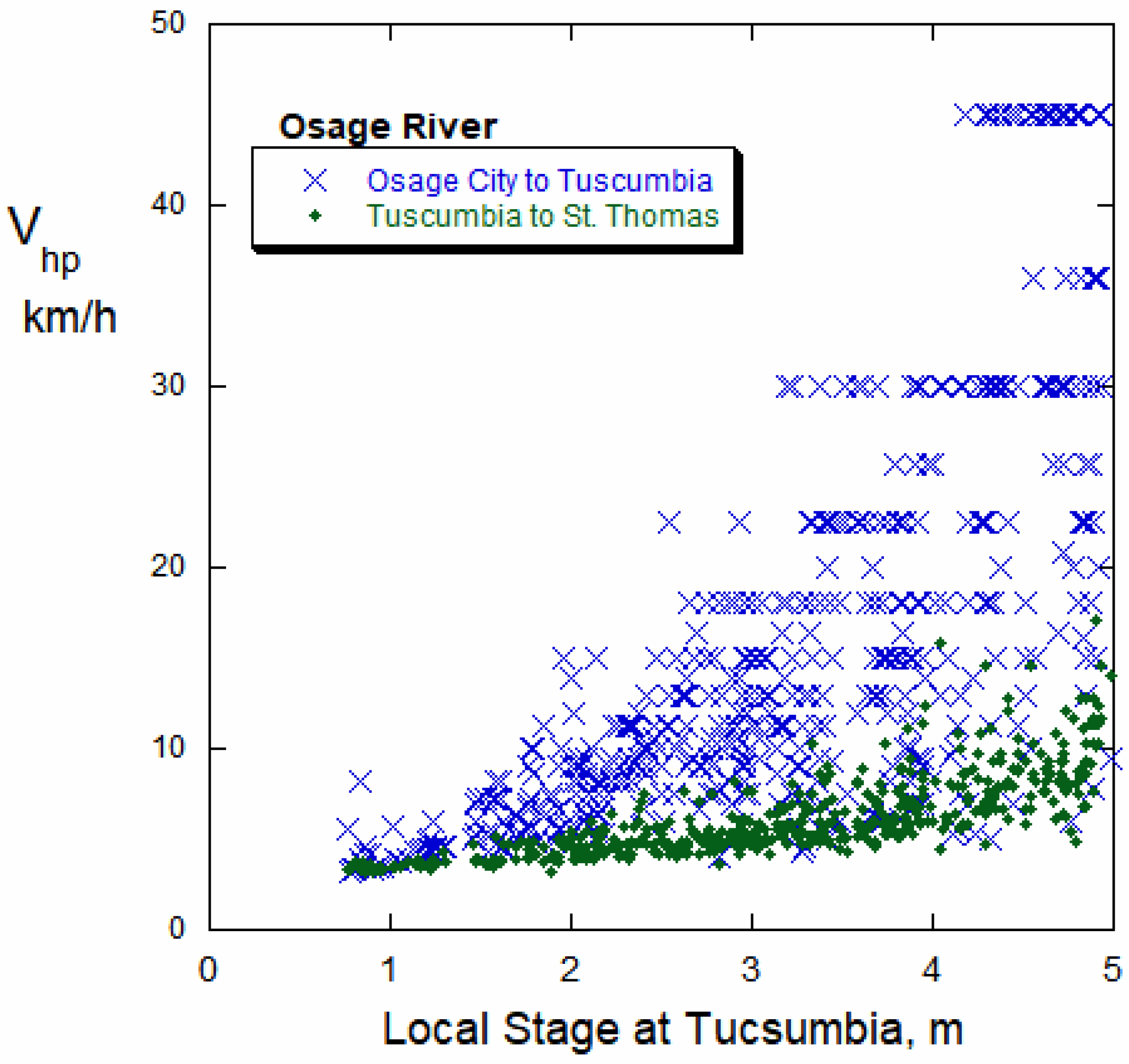
The observed velocity of hydropower peaks along the Osage River correlates positively with river stage. This is shown for the reach between the Osage City gauge and the Tuscumbia gauge, located 22.5 km apart, and also for the reach between Tuscumbia and the St. Thomas gauge, located 51.3 km mi apart. Because the difference between local stage and water depth is small for the Osage River gauges (small S0 estimates in Table 1), rendering the uncertainty rather large compared to the size of the suggested correction, no correction to local stage was made in Figure 3, so the trends cannot be expected to project perfectly to the origin. Also, the correlations shown are similar and could be improved if various linear combinations were made of the stages at the various gauges, so the measured, uncorrected stage at Tuscumbia is used for simplicity on the x-axis in this plot. Also note that as stage increases, the relative differences (scatter) among the Vhp values increase. This is partly because the faster the peak moves downstream, the greater the relative uncertainty in timing caused by the 15 min data interval. For example, the fastest peaks arrive at Tuscumbia only a single, 15 min time step after they pass the Osage City gauge, so the Vhp values calculated for this case would be uncertain by a factor of two.
The data in Figure 3 do not conform to the standard expectation of Equation (1) that celerity c increases with the square root of water depth, as such a trend would have downward curvature on this plot. Specifically, the correlation of Vhp with the stage at Tuscumbia has a strong positive curvature. In fact, available data show that the average velocity of water in many Midwestern river channels increases linearly with water depth [33], but not in the manner predicted by the Chezy or Manning equations or in a manner consistent with Equation (1).
4.2.3. Peak Attenuation, Osage River
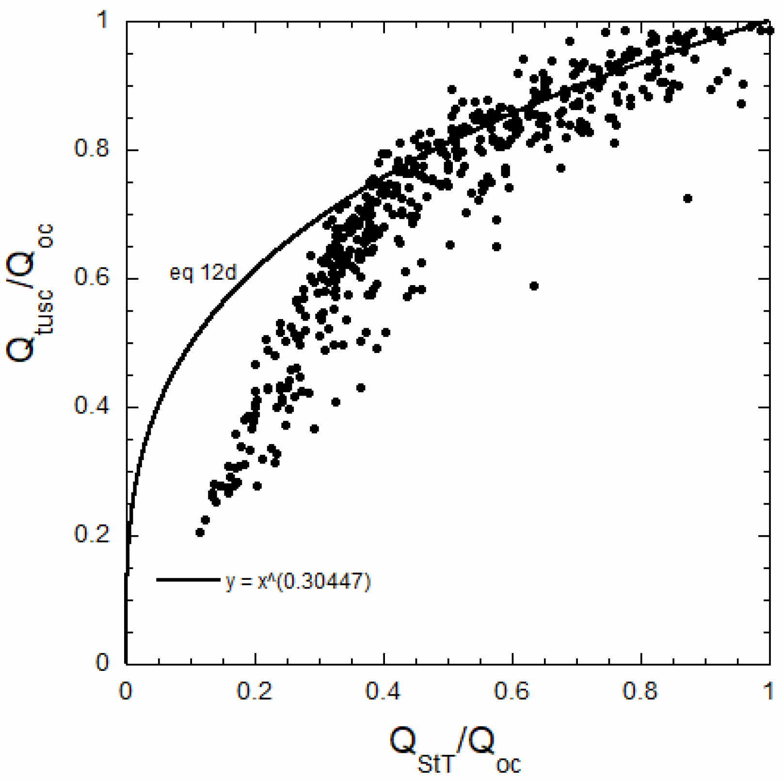
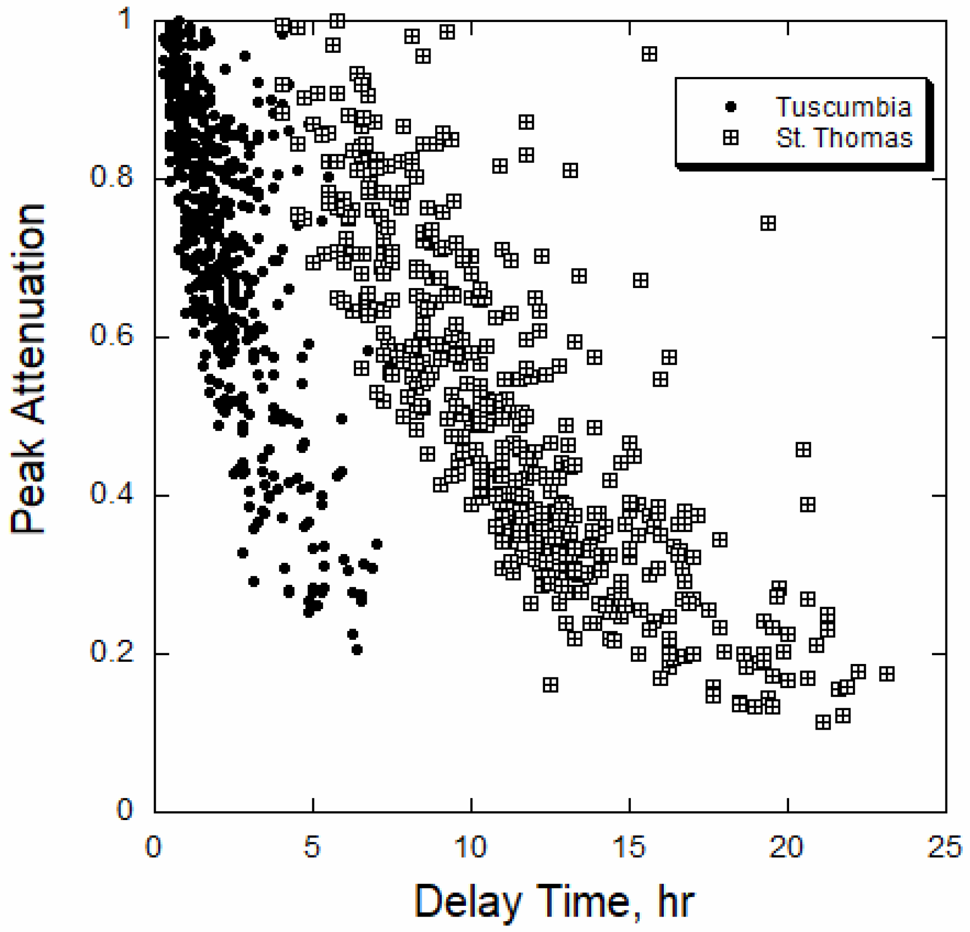
Hydropower flow peaks become lower and wider with increasing distance and travel times below dams. On the Osage River, the fractional loss of peak discharge magnitude between Osage City and Tuscumbia, corrected for the minimum flow at Osage City, is strongly correlated with the greater fractional loss between Osage City and St. Thomas (Figure 4). The data trend conforms well with Equation (12d), which predicts that the ratio of the inter-site distances, which for this case is 22.5/73.9, is the relevant power. Highly attenuated flows diverge from this line, in part because these are most sensitive to the background correction, are most dependent on the accuracy of the rating curves, and are most dependent on variable tributary inflows. The fractional losses also correlate with several other factors, including the travel time of the peak (Figure 5), which is inversely related to peak velocity. As mentioned above, peak velocity in turn depends on water depth and the duration of the causal pulse.
4.2.4. Comparison of Osage River Data with Convolution Integral
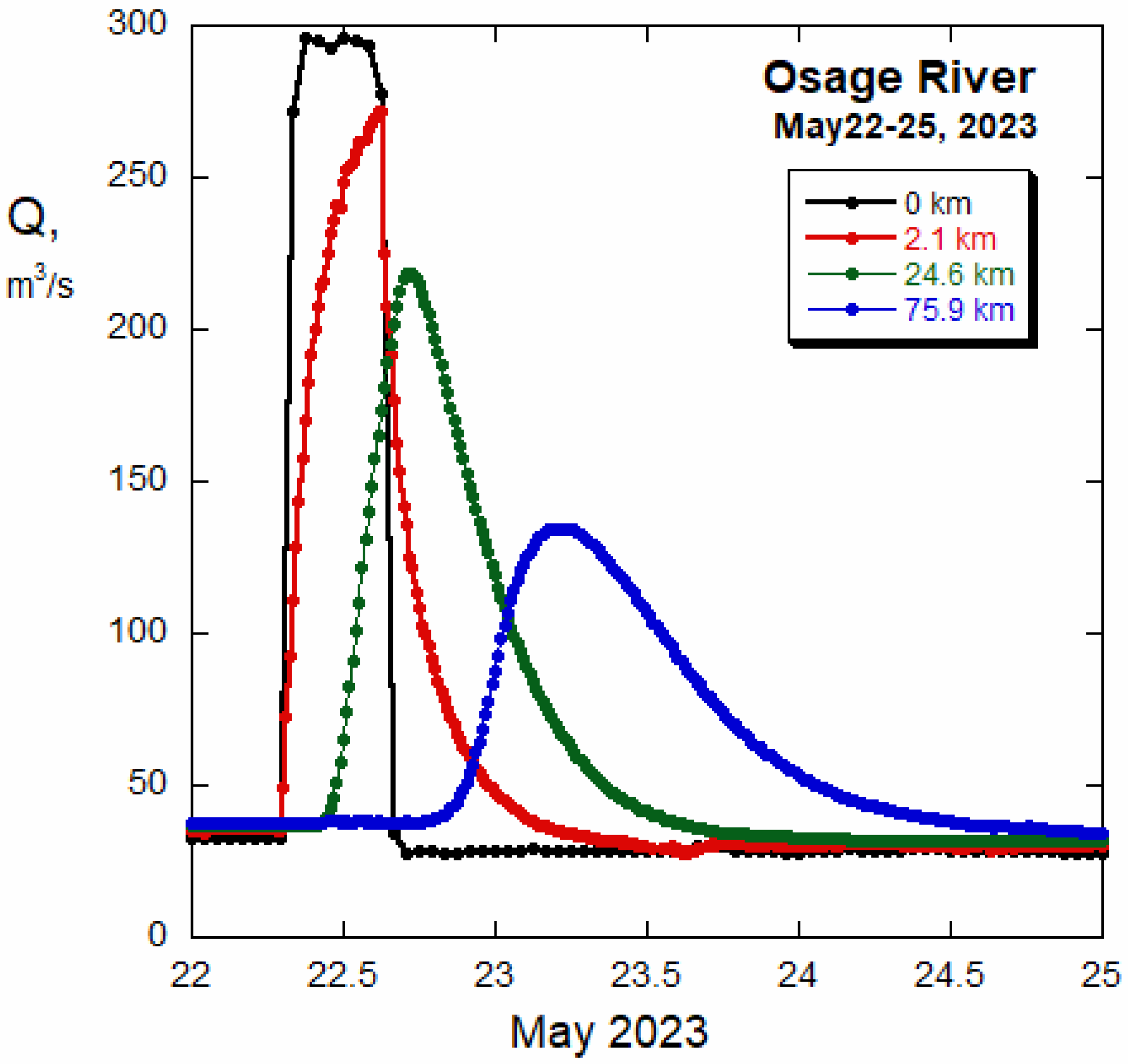
The shapes of Osage River hydrographs qualitatively resemble those provided by the convolution integrals of the diffusion-advection equation (Figure 2B), but their agreement with predicted quantitative details is only fair. An example from May 2023 was selected for this comparison because the initial pulse released from the dam approximated the rectangular shape assumed in those integrals, had a modest height, and was superimposed on low river flow. Examination of large flow peaks is not optimal due to the greater uncertainty of Vhp values for such events (Figure 3).
In particular, the Osage River hydrographs (Figure 6) evolve and attenuate downstream in the general way indicated by Equation (11a,b) and Figure 2B. Parameter combinations can doubtless be found where the latter closely resemble the data for any individual gauge, but little would be gained here from individualized, ad hoc curve matching. No single set of parameter choices, along with the known distances and the known τ values, can accurately explain the May 2023 data for all four sites. For example, peak velocities are much higher at Osage City than downstream (Figure 3), so using a single value of celerity for all reaches is inappropriate. It is also likely that changes in channel character with distance affect the site-specific parameter values. For example, the channel width just below the dam is much wider than that typical downstream. As a result, the hydraulic diffusivity for the reach between Bagnell dam and the Osage City gauge would be lower than that downstream because the channel storage is higher, and diffusivity indicates the ratio of transmissivity to storativity. A detailed study would be required to determine whether the various parameters vary with flow conditions, in which case, the actual differential equation would be non-linear and much more complicated than the underlying differential equation (Equation (9)) assumed here, and the convolution problem would be impossible to solve in closed form with known analytical methods.
4.3. Comparison with Flood Hydrographs
Natural flood waves are driven by precipitation, which is aggregated in tributaries that contribute flow to the trunk river channel. The behavior of the flood peaks depends on the amounts and spatial and temporal distribution of rainfall delivered to the watershed, the transport mechanisms and rates of surface and subsurface runoff, and the locations of the sub-watersheds and confluences of the various tributaries. Additional complexities are introduced by overbank flows, levee breaks, etc. If the river is a tributary of a larger river that is also undergoing flooding, flows in its lower reaches can be retarded or even reversed, and under backwater conditions, peak arrivals at multiple sites can be nearly simultaneous.
The propagation rate of typical, individual flood peaks (Vnflood) created by rainfall events is easily determined by plotting the thalweg distance of different stream gauges against the peak arrival times. For rivers where multiple gauges are available, the trend lines for some floods are almost linear, indicating that peak velocities remain nearly constant, even as the slopes of both the channel bottom and the water surface flatten downstream. Interestingly, the peak velocities (Vrflood) of huge record floods of rivers progress more slowly than typical floods, with available data showing that they typically are even slower than the average velocity (Vravg) of channel water during those record events (Table 3). This is likely due to the contributions of slow, shallow overbank flows and the greatly increased storage of water on and below the inundated floodplains (cf. [21,22]).
In contrast to the progressive attenuation of hydropower peaks or dam breaks, the peak discharges of natural, rainfall-driven floods typically increase downstream. In fact, except for rare losing streams, the mean, median, and record flows of rivers all increase downstream, in proportion to some power of the basin area, which must increase downstream [38]. Only in the special case where heavy precipitation occurs in the headwaters or upper reaches while dry conditions prevail in the lower basin can peak discharges of natural floods on normal rivers decrease downstream.
Processing of multiyear data along the same rivers (see Section 2) confirms that typical flood peaks move more rapidly than the peaks of record floods (Table 3). Considering all the data together, this study finds that the hierarchy of the various flow velocities is as follows:
Vhp ~ c > Vnflood > Vavg > Vrflood.
Table 3.
Propagation speeds of normal and record flood peaks compared to the average water velocity measured for the record flood.
Table 3.
Propagation speeds of normal and record flood peaks compared to the average water velocity measured for the record flood.
| River | Distance km | Slope m/km | Tortuosity | Vnflood * m/s | Vravg † m/s | Vrflood ‡ m/s | Reference ‡ |
|---|---|---|---|---|---|---|---|
| Middle Mississippi, 1993 | 219 | 0.095 | 1.30 | 2.1 | 2.1 | 0.42 | [20] |
| Lower Missouri, 1993 | 860 | 0.17 | 1.70 | 2.2 | 2.1 | 1.1 | This paper |
| Yellowstone, 2022 | 871 | 1.14 | 1.44 | 1.9 | 2.6 | 1.6 | This paper |
| Meramec, 2015 | 291 | 0.47 | 2.76 | 1.3 | 1.4 | 0.85 | [39] |
| Upper River des Peres, 2022 | 5.5 | 2.44 | 1.35 | 2.3 | 2.4 | 1.1 | [40] |
Note(s): * Results for several floods since 2020, whose peaks were tracked over the thalweg distance given in the second column. † Measured average water velocity from USGS field data [27] for the record flood only, whose year is given in the left column. ‡ Propagation rate for the record flood peak based on its arrival at multiple gauges, per indicated reference.
5. Discussion
The results documented above are based on the systematic processing of several million measurements of river stages, most gathered at 15 min intervals and accompanied by estimated discharge, representing 60 monitored sites used in Table 1 and Table 3. An unexpected richness of dynamic behaviors was revealed when these results were compared to each other, to various site characteristics, to well-known theoretical results, and to the new solutions and approximations to the diffusion-advection equation.
The diffusion-advection equation is clearly capable of simulating realistic hydrograph shapes below hydropower dams. This equation also reveals the major variables that control peak attenuation, and an important new finding is that this strongly depends on the duration of the source pulse. It follows that the short list of variables, parameters, and specific derivatives embodied in the diffusion-advection equation, together with convolution integrals for appropriate source pulse shapes, describe the most important behaviors of hydropower waves.
Perhaps the most surprising finding is the hierarchy of different velocity types codified in Equation (13). This hierarchy is only partly consistent with theoretical expectations for these velocities, now discussed from fastest to slowest. First, hydropower peaks move in a small excess of celerity, especially just below dams, because diffusion effects also contribute to the peak velocity, as seen in Approximation (12b). Clearly, diffusion alone can cause some peak propagation, as evident in Figure 2A.
Second, celerity exceeds the average velocity of channel water, as is well known and predicted by both Equations (1) and (2). It is also well known from weirs, etc. that the average velocity of channel water increases with the stage. Thus, the behavior of record flood peaks is very surprising, because even though flood water levels are very high, these huge peaks typically move more slowly than the average velocity of water in the channel. It appears that natural flood peaks move more slowly the bigger they are, so the higher and deeper the water, the slower they are, contrary to average channel velocity. The likely explanation is that precipitation must move overland and underground to reach the channel, and the associated mechanisms of delivering water to the channel differ from the movement of water down the channel. Tributary effects, overbank flows, and details of rainfall delivery provide many additional complications to the behavior of natural floods.
Another surprise is the weak dependence of peak velocities on channel slope. It is as if hydropower pulses acquire a momentum of their own and that these masses then move at a constant bulk velocity that is independent of the localized accelerations produced by channel variations. Indeed, conservation of momentum might explain this behavior of hydropower pulses, which widen and flatten but do not gain mass as they travel. Again, the behavior of most natural floods is far more complex than hydropower pulses, as the total mass of floodwater greatly increases with downstream distance.
The correlation between pulse speed and tortuosity is new and requires more study. As mathematically defined, tortuosity is the ratio of the lengths of an arc to its cord, and in physical studies, it is the ratio of the actual path (or channel) length to the direct distance. Tortuosity is easier to consistently define than river sinuosity, which is a similar quantity defined as the ratio of channel length to the length of the valley [41].
Finally, the differential equations used in this report require comment. The diffusion and diffusion-advection equations are widely used in physics, chemistry, and engineering to simulate the transfer of heat or matter. The hydrologic diffusion equation (Equation (4)) embodies analogous principles as it describes the diffusion of hydraulic head h, which is proportional to the energy per unit mass. In contrast, Equation (9) describes the combined diffusive-advective transport of discharge (Q), which is a flux. Temperature, concentration, and head are routinely analyzed with the diffusion and diffusion-advection equations, but these quantities represent amounts, and amounts are fundamentally different than fluxes, which involve the derivatives of amounts. Sources cited above argue that Equation (9) is applicable to channel flow, but its difference with the conventional diffusion-advection equation requires more study. Additional problems arise for any of these equations if the celerity or diffusivity are not simple constants along the channel, as seems to be the case for the Osage River. Non-linear differential equations are needed to describe the dynamic behavior of such systems, and analytical solutions are probably impossible. These issues may explain some of the differences between real rivers and the idealized predictions of the convolution integrals.
Future Work
The rich database of river gauge observations that is now available is underutilized. Only 25 years ago, compiling gauge data needed for river analysis required weeks of tedious searches of library catalogs, but such data can now be acquired in a few hours from online sources. The massive amount of data in these online resources (e.g., [3,27,42]) represents many man-centuries of sustained, commendable efforts to document river behavior and provides the means to test both models and theories. As an example, such data demonstrate that Manning’s equation does a poor job of simulating actual field measurements of average channel velocity in rivers [33], yet Manning’s equation is central to the HEC-RAS algorithm [43]. Perhaps this explains why the FEMA’s probabilistic stage-discharge pairs for St. Louis streams [44], which are based on HEC-RAS calculations, differ from the on-line USGS rating curves [27] for most of the same sites, sometimes by a factor of two.
Commendable though it is, the river gauge data base can be improved. The current redaction of pre-2008 or even pre-2016 stage measurements from the online USGS database is unjustified, as stage is the measurement that is most accurately made and is the one that is most relevant to flood risk. The documentation of gauged sites is also inadequate, and even the posted values for “gauge zero” are sometimes inaccurate and, in the worst cases, would even suggest that water flows uphill [31], yet these values are needed to convert local stages to elevations. Channel cross-sections that include bathymetric profiles are needed for every gauged site and would greatly further the understanding of river dynamics and the improvement of rating curves. Moreover, the important phenomenon of stage-discharge hysteresis, of which convincing examples are abundant (e.g., [19,33,45]), is not accommodated by USGS rating curves and by ratings based on HEC-RAS.
The convolution integral problem outlined here should be solved for different shapes of the source pulse. For example, it seems likely that dam releases featuring a slow, linear initial ramp would progress more slowly and be less destructive and erosive than those featuring the sudden ramp-up of the rectangular pulse. Perhaps the aquatic ecosystem would benefit from a highly varied pattern of pulse shapes on successive days. In short, quantifying a larger class of these behaviors could provide new insights on river dynamics while suggesting valuable ways to improve dam management.
More exact, closed-form analytical solutions to the equations of river dynamics are needed. Though analytical solutions are possible only for idealized, simplified situations, they provide fundamental insights, have great educational value, and precisely quantify the endmember cases needed to test and improve numerical algorithms. The use of the exponential integral in the “well equation” [46] and the extension of solutions to Laplace’s equation to regional groundwater flow [47] revolutionized the understanding and visualization of groundwater processes. These idealized solutions are widely used, grace numerous textbooks, and are fundamentally grounded in the simplest terms of transport theory.
6. Conclusions
This paper shows that the diffusion-advection equation describes the major dynamic behaviors and evolution of flow pulses released by hydropower dams, including their basic shapes, propagation speeds, and attenuation. Considering these pulses simplifies the analysis of natural flood waves, as hydropower pulses arise from a single source and their subsequent behavior depends only on channel conditions and character and not on flow augmentations by tributaries or variable rainfall. This study confirms that hydropower pulses move downstream at a nearly constant rate that exceeds the average velocity of water in the channel. Hydropower peak velocities tend to increase with water level, as does the average velocity of channel water, and appear to decrease with increasing channel tortuosity and to increase weakly with channel slope. Peak flows attenuate in an approximately exponential manner with downstream distance as peak shapes flatten, widen, and become smoother and more symmetrical. This study also shows, and confirms with data, that attenuation also increases as travel times become longer. Hence, between two sites, small, slow-moving flow peaks diminish proportionally more than large, fast-moving peaks. Another new finding is that attenuation diminishes as the duration of the source pulse increases. Many of these basic behaviors are explained by the convolution integral of the fundamental solution of the hydraulic diffusion-advection equation and, in particular, by the exact expression for the dynamic evolution of a “rectangular” source pulse that is provided here.
Natural, precipitation-driven flood waves are affected by factors in addition to channel character, especially by the spatial and temporal variations in rainfall delivery and by the complicated paths and mechanisms that deliver this water to the trunk river. Unlike hydropower pulses, the heights and discharges of most natural flood peaks increase downstream rather than attenuate. Surprisingly, the propagation speeds of natural flood peaks tend to decrease with stage and become quite slow for huge floods. Part of this delay may be due to storage effects in overbanked areas. Moreover, for natural floods, the slow transport of runoff across and beneath the entire watershed is probably much more important than the simple flow of water down the channel.
A comparison of theoretical results and observational data suggests the following rich hierarchy of different velocities that define the dynamics of river water waves:
Vhp ~ c > Vnflood > Vavg > Vrflood
Finally, the flow releases of hydropower dams are usefully considered a type of “water mining”, as these releases extract potential energy from the water via a process that degrades water quality and riverine ecosystems.
Funding
This research received no external funding.
Data Availability Statement
All data are publicly available; most data are present in [27].
Acknowledgments
I thank David L. Nelson and Anne M. Hofmeister for valuable discussion, and Hugh Chou and Washington University for computer support.
Conflicts of Interest
The author declares no conflicts of interest.
References
- Chow, V.T. Handbook of Applied Hydrology; McGraw-Hill: New York, NY, USA, 1964. [Google Scholar]
- U.S. Department of Agriculture, Flood Routing. Chapter 17, National Engineering Handbook, Part 630. 2014. Available online: https://damtoolbox.org/images/a/a6/NEH17.pdf (accessed on 20 February 2024).
- National Weather Service, Advanced Hydrologic Prediction Service (AHPS). Available online: https://water.weather.gov/ahps/ (accessed on 20 March 2024).
- Ferrick, M.G. Analysis of River Wave Types. Water Resour. Res. 1985, 21, 209–220. [Google Scholar] [CrossRef]
- Kocaman, S.; Evangelista, S.; Guzel, H.; Dal, K.; Yilmaz, A.; Viccione, G. Experimental and Numerical Investigation of 3D Dam-Break Wave Propagation in an Enclosed Domain with Dry and Wet Bottom. Appl. Sci. 2021, 11, 5638. [Google Scholar] [CrossRef]
- Kalinina, A.; Spada, M.; Vetsch, D.F.; Marelli, S.; Whealton, C.; Burgherr, P.; Sudret, B. Metamodeling for Uncertainty Quantification of a Flood Wave Model for Concrete Dam Breaks. Energies 2020, 13, 3685. [Google Scholar] [CrossRef]
- Psomiadis, E.; Tomanis, L.; Kavvadias, A.; Soulis, K.X.; Charizopoulos, N.; Michas, S. Potential Dam Breach Analysis and Flood Wave Risk Assessment Using HEC-RAS and Remote Sensing Data: A Multicriteria Approach. Water 2021, 13, 364. [Google Scholar] [CrossRef]
- Criss, R.E.; Hofmeister, A.M. Can Modern Science Answer the Great Questions? J. Earth Science 2022, 33, 1330–1332. [Google Scholar] [CrossRef]
- Carslaw, H.S.; Jaeger, J.C. Conduction of Heat in Solids; Clarendon Press: Oxford, UK, 1959. [Google Scholar]
- Ponce, V.M. Generalized diffusion wave equation with inertial effects. Water Resour. Res. 1990, 26, 1099–1101. [Google Scholar] [CrossRef]
- Yen, B.C.; Tsai, C.W.S. On noninertia wave versus diffusion wave in flood routing. J. Hydrol. 2001, 244, 97–104. [Google Scholar] [CrossRef]
- Brutsaert, W. Hydrology, an Introduction; Cambridge University Press: New York, NY, USA, 2005; p. 618. [Google Scholar]
- Kazezyılmaz-Alhan, C.M.; Medina, M.A. Kinematic and Diffusion Waves: Analytical and Numerical Solutions to Overland and Channel Flow. J. Hydraul. Eng. 2007, 133, 217–227. [Google Scholar] [CrossRef]
- Fenton, J.D. Flood routing methods. J. Hydrol. 2019, 570, 251–264. [Google Scholar] [CrossRef]
- Criss, R.E.; Winston, W.E. Discharge predictions of a rainfall-driven theoretical hydrograph compared to common models and observed data. Water Resour. Res. 2008, 44, W10407. [Google Scholar] [CrossRef]
- Yang, Y.; Endreny, T.A. Watershed hydrograph model based on surface flow diffusion. Water Resour. Res. 2013, 49, 507–516. [Google Scholar] [CrossRef]
- Whitham, G.B. Linear and Nonlinear Waves; John Wiley & Sons: New York, NY, USA, 1974; 636p. [Google Scholar]
- Bascomb, W. Waves and Beaches; Doubleday and Co.: Garden City, NY, USA, 1964. [Google Scholar]
- Faye, R.E.; Cherry, R.N. Channel and Dynamic Flow Characteristics of the Chattahoochee River, Buford Dam to Georgia Highway 141; U.S. Geological Survey Water-Supply Paper, 2063; U.S. Government Printing Office: Washington, DC, USA, 1980. [Google Scholar]
- Moody, J.A. Propagation and composition of the flood wave on the upper Mississippi River, 1993. USGS Circ. 1993, 1120, 1–21. [Google Scholar]
- Wong, T.H.; Laurenson, E.M. Wave speed-discharge relations in natural channels. Water Resour. Res. 1983, 19, 701–706. [Google Scholar] [CrossRef]
- Meyer, A.; Fleischmann, A.S.; Collischonn, W.; Paiva, R.; Jardim, P. Empirical assessment of flood wave celerity discharge relationships at local and reach scales. Hydrol. Sci. J. 2018, 63, 2035–2047. [Google Scholar] [CrossRef]
- Clarence Cannon Dam. Available online: https://marktwain.uslakes.info/DamInfo.asp?DamID=69009941-FA37-49FC-ACD4-ED100484476A (accessed on 20 March 2024).
- Cushman, R.M. Review of Ecological Effects of Rapidly Varying Flows Downstream from Hydroelectric Facilities. N. Am. J. Fish. Manag. 1985, 5, 330–339. [Google Scholar] [CrossRef]
- Ashby, S. Impacts of hydrology and hydropower on water quality in reservoir tailwaters. WIT Trans. Ecol. Environ. 2009, 124, 55–66. [Google Scholar]
- USACE. Missouri River Stage Trends, Technical Report; USACE: Winchester, VA, USA, 2012; 46p. [Google Scholar]
- U.S. Geological Survey Current Water Data for the Nation. Available online: https://waterdata.usgs.gov/nwis/rt (accessed on 20 March 2024).
- National Weather Service. Rivers of the US. Available online: https://www.weather.gov/gis/Rivers (accessed on 20 March 2024).
- United States Census. Cartographic Boundary Files-Shapefile. Available online: https://www.census.gov/geographies/mapping-files/time-series/geo/carto-boundary-file.html (accessed on 20 March 2024).
- MSDIS Missouri Spatial Data Information Service, State-Extent DEM. Available online: https://www.msdis.missouri.edu/data/elevation/index.html (accessed on 20 March 2024).
- Criss, R.E.; Nelson, D.L. Discharge-stage relationship on urban streams evaluated at USGS gauging stations, St. Louis, Missouri. J. Earth Sci. 2020, 31, 1133–1141. [Google Scholar] [CrossRef]
- Criss, R.E. The Hydrologic Time Scale: A Fundamental Stream Characteristic. J. Earth Sci. 2022, 33, 1291–1297. [Google Scholar] [CrossRef]
- Criss, R.E. Dependence of discharge, channel area, and flow velocity on river stage and a refutation of Manning’s equation. Geol. Soc. Am. Spec. Pap. 2022, 553, 193–199. [Google Scholar]
- Domenico, P.A.; Schwartz, F.W. Physical and Chemical Hydrogeology; John Wiley & Sons: New York, NY, USA, 1990. [Google Scholar]
- Criss, R.E.; Winston, W.E. Hydrograph for small basins following intense storms. Geophys. Res. Lett. 2003, 30, 1314–1318. [Google Scholar] [CrossRef]
- Criss, R.E. Theoretical Link between Rainfall and Flood Magnitude. Hydrol. Process. 2018, 22, 1607–1615. [Google Scholar] [CrossRef]
- Osage Headwater and Tailwater Report. Available online: https://apps.ameren.com/HydroElectric/Reports/Osage/HeadWaterTailWater.aspx (accessed on 20 February 2024).
- Winston, W.E.; Criss, R.E. Dependence of Mean and Peak Streamflow on Basin Area in the Conterminous United States. J. Earth Sci. 2016, 27, 83–88. [Google Scholar] [CrossRef]
- Criss, R.E.; Luo, M. River management and flooding: The lesson of December 2015–January 2016, Central USA. J. Earth Sci. 2016, 27, 117–122. [Google Scholar] [CrossRef]
- Criss, R.E.; Stein, E.M.; Nelson, D.L. Generation and Propagation of an Urban Flash Flood and Our Collective Responsibilities. J. Earth Sci. 2022, 33, 1624–1628. [Google Scholar] [CrossRef]
- Schumm, S.A. Sinuosity of Alluvial Rivers on the Great Plains. Geol. Soc. Am. Bull. 1963, 74, 1089–1100. [Google Scholar] [CrossRef]
- RiverGages.com. Available online: https://rivergages.mvr.usace.army.mil/WaterControl/new/layout.cfm (accessed on 20 March 2024).
- HEC-RAS Hydraulic Reference Manual. Available online: https://www.hec.usace.army.mil/confluence/rasdocs/ras1dtechref/latest (accessed on 20 March 2024).
- FEMA. Flood Insurance Study; Study Number 29889CV001A; FEMA: St. Louis, MO, USA, 2015; Volume 1–4. [Google Scholar]
- Muste, M.; Dongsu, K.; Kyungdon, K. Insights into flood wave propagation in natural streams as captured with acoustic profilers at an index-velocity gaging station. Water 2022, 14, 1380. [Google Scholar] [CrossRef]
- Theis, C.V. The relation between the lowering of the Piezometric surface and the rate and duration of discharge of a well using ground-water storage. Trans. Amer. Geophys. Union 1935, 2, 519–524. [Google Scholar] [CrossRef]
- Toth, J. A theoretical analysis of groundwater flow in small drainage basins. J. Geophys Res. 1963, 68, 4795–4812. [Google Scholar] [CrossRef]
Figure 1.
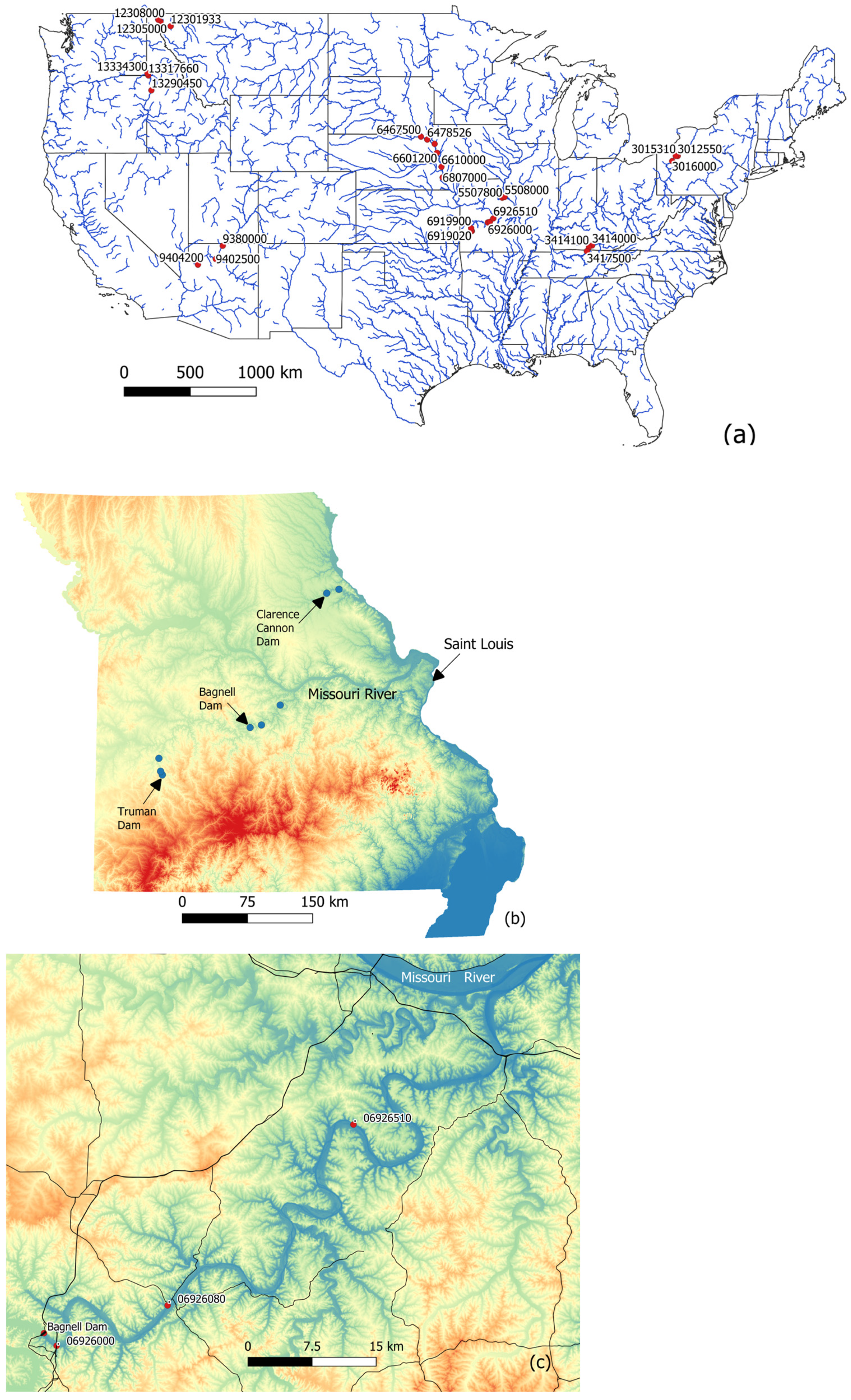
(a) Map showing major rivers in the United States [28,29] and the location (red dots) of the river gauges listed in Table 1. The initial zero is omitted from several site numbers, and 3 sites cannot be labeled for clarity. (b) Digital elevation map (DEM) of Missouri [30] in the central United States, showing the Bagnell, Truman, and Clarence Cannon Dams on the Osage, Sac, and Salt Rivers, respectively, and the river gauges (blue dots; Table 1) below those dams. (c) A detailed map showing major roads, the Bagnell Dam, and the three river gauges (red dots) along the Osage River in Missouri that were selected for detailed study.
Figure 1.
(a) Map showing major rivers in the United States [28,29] and the location (red dots) of the river gauges listed in Table 1. The initial zero is omitted from several site numbers, and 3 sites cannot be labeled for clarity. (b) Digital elevation map (DEM) of Missouri [30] in the central United States, showing the Bagnell, Truman, and Clarence Cannon Dams on the Osage, Sac, and Salt Rivers, respectively, and the river gauges (blue dots; Table 1) below those dams. (c) A detailed map showing major roads, the Bagnell Dam, and the three river gauges (red dots) along the Osage River in Missouri that were selected for detailed study.

Figure 2.
(A) Graphs of flow vs. time for various choices of the time constant b, calculated with Equation (8a,b) for diffusion only. The curve for b = 0 represents the rectangular, unit flow pulse that issues from the source (dam), while the curves for increasing values of b simulate the flow variations at increasing distances downstream. (B) Flows calculated with Equation (11a,b) that incorporate both celerity and diffusion for different indicated distances.

Figure 3.
Propagation velocities (Vhp) of the 494 hydropower flow peaks for each of two reaches along the Osage River plotted against the observed, uncorrected, local stage of those flow peaks at the Tuscumbia gauge. Six points for the Osage City to Tuscumbia reach (X’s) are offscale.
Figure 3.
Propagation velocities (Vhp) of the 494 hydropower flow peaks for each of two reaches along the Osage River plotted against the observed, uncorrected, local stage of those flow peaks at the Tuscumbia gauge. Six points for the Osage City to Tuscumbia reach (X’s) are offscale.

Figure 4.
Comparison of the peak discharges at Tuscumbia (Qtusc) and St. Thomas (QStT), each normalized to the peak discharge at Osage City (Qoc), all corrected for the minimum discharge at Osage City prior to each pulse event. The proportional losses (attenuation) at St. Thomas are greater than those at Tuscumbia. The solid curve shows the trend predicted by Equation (12d). Of the 494 pulse events selected for study, 20 are offscale.

Figure 5.
Peak attenuation at Tuscumbia (dots) and at St. Thomas (squares) relative to peak size at Osage City, plotted against the travel time of the peaks between each site and Osage City. Peak flows become more attenuated as travel time increases, as predicted by Equation (12a), assuming that the travel time is related to distance divided by celerity. Twenty pairs of points are offscale.

Figure 6.
Hydrographs at Osage City (red; 2.1 km; USGS 06926000), Tuscumbia (green; 24.6 km; USGS 06926080), and St. Thomas (blue; 75.9 km; USGS 06926510), driven by the 8 h, rectangular flow pulse of 22 May 2023 released from Bagnell Dam (black; 0 km; Ameren 2023). The USGS gauge data [27] are reported at 15 min intervals, but the Ameren data [37] are hourly. Note the progressive attenuation and delay of the peaks with distance downstream of Bagnell Dam. Compare these data with the theoretical predictions in Figure 2B for similar thalweg distances and source pulse durations.

Table 2.
Dependence of peak character on model parameters.
| Factor | Peak Velocity | Attenuation | Peak Shape |
|---|---|---|---|
| Greater distance | Slower | More | More symmetrical |
| Longer τ | Faster | Less (strong) | Ditto |
| Higher c | Faster (strong) | Less | Ditto |
| Larger κ | Faster | Less (weak) | Less symmetrical |
Disclaimer/Publisher’s Note: The statements, opinions and data contained in all publications are solely those of the individual author(s) and contributor(s) and not of MDPI and/or the editor(s). MDPI and/or the editor(s) disclaim responsibility for any injury to people or property resulting from any ideas, methods, instructions or products referred to in the content. |
© 2024 by the author. Licensee MDPI, Basel, Switzerland. This article is an open access article distributed under the terms and conditions of the Creative Commons Attribution (CC BY) license (https://creativecommons.org/licenses/by/4.0/).
Share and Cite
MDPI and ACS Style
Criss, R.E. Dynamics of River Flood Waves below Hydropower Dams and Their Relation to Natural Floods. Water 2024, 16, 1099. https://doi.org/10.3390/w16081099
AMA Style
Criss RE. Dynamics of River Flood Waves below Hydropower Dams and Their Relation to Natural Floods. Water. 2024; 16(8):1099. https://doi.org/10.3390/w16081099
Chicago/Turabian StyleCriss, Robert E. 2024. "Dynamics of River Flood Waves below Hydropower Dams and Their Relation to Natural Floods" Water 16, no. 8: 1099. https://doi.org/10.3390/w16081099
Note that from the first issue of 2016, this journal uses article numbers instead of page numbers. See further details here.